彈性分封環之高效能乏晰公平流速產生器

國 立 交 通 大 學

電信工程學系

碩 士 論 文

彈性分封環之高效能乏晰公平

流速產生器

An Effective Fuzzy Local Fair Rate

Generator for Resilient Packet Ring

研 究 生：王維謙

指導教授：張仲儒 博士

彈性分封環之高效能乏晰公平流速產生器

An Effective Fuzzy Local Fair Rate Generator

for Resilient Packet Ring

研 究 生：王維謙 Student：Wei-Chien Wang

指導教授：張仲儒 博士 Advisor：Dr. Chung-Ju Chang

國立交通大學

電信工程學系

碩士論文

A Thesis

Submitted to Department of Communication Engineering

College of Electrical and Computer Engineering

National Chiao Tung University

in Partial Fulfillment of the Requirements

for the Degree of Master of Science

in

Communication Engineering

July 2008

Hsinchu, Taiwan

彈性分封環之高效能乏晰公平流速產生器

研究生：王維謙 指導教授：張仲儒

國立交通大學電信工程系碩士班

摘要

彈性分封環(Resilient Packet Ring)是一種應用於高速都會區域網路的環狀 網路架構，並且擁有容錯與高頻寬使用率等特性。在彈性分封環中，公平性、穩 定性、和收斂時間等在壅塞控制中是很重要的議題。在本篇論文中，我們提出一 個高效能乏晰公平流速產生器(FLFRG)，藉著乏晰運作機制產生一個準確的本地 公平流速來抑制壅塞情況並且達成上述考量。所提出的機制，是由三個部份所組 成，適應性公平流速計算器(AFRC)、乏晰壅塞偵測器(FCD)、與乏晰公平流速計 算器(FFRC)。適應性公平流速計算器產生一個評估過的公平流速而乏晰壅塞偵測 器根據次級傳輸緩衝器(STQ)的容納量與接收到的流量大小來指出當前的壅塞程 度。乏晰公平流速計算器經由考量兩項由適應性公平流速計算器與乏晰壅塞偵測 器輸出的結果來得到反映真實流量狀況的本地公平流速。藉由適應性公平流速計 算器與乏晰壅塞偵測器的使用，乏晰公平流速產生器可產生較小的收斂時間，再 者當與其它演算法相比，在不同大小的壅塞區域中皆獲得極好的效果。模擬結果 顯示出我們所提出的方法，不管在公平性、穩定性、與收斂時間都上擁有傑出的 效果。因此乏晰公平流速產生器不失為一個具可行性且十分吸引人的方法。

An Effective Fuzzy Local Fair Rate Generator

for Resilient Packet Ring

Student: Wei-Chien Wang Advisor: Chung-Ju Chang

Department of Communication Engineering

National Chiao Tung University

Abstract

The resilient packet ring (RPR) is a ring based network for high-speed metropolitan area networks which has properties of fault tolerance and high bandwidth utilization. In RPR, the issues of fairness, stability, and convergence time are important in congestion control. In this thesis, we propose an effective fuzzy local fair rate generator (FLFRG) to achieve above considerations. FLFRG generates a precise local fair rate by fuzzy logics to suppress upstream traffic causing congestion. FLFRG is composed of three components: adaptive fair rate calculator (AFRC), fuzzy congestion detector (FCD), and fuzzy fair rate calculator (FFRC). AFRC produces an estimated fair rate and FCD indicates the congestion degree of local station according to STQ occupancy and arrival rate to STQ. FFRC adopts the two outputs of AFRC and FCD to generate a local fair rate which reflects the real traffic condition. Since AFRC and FCD are applied, the smaller convergence time than other fairness algorithms is obtained. Furthermore, even in different scales of congestion domain, FLFRG still has an excellent performance as compared with other fairness algorithms. Simulation results show that the proposed FLFRG has an outstanding performance on fairness, stability, and convergence time in different testing scenarios. Consequently, we can conclude that the FLFRG is a feasible and attractive design for congestion control in RPR.

誌 謝

此篇論文得以完成，首先我要感謝指導教授張仲儒博士，沒有他引導自己的 論文方向，沒有他在撰稿細節上的提醒，論文無法順利完成。在論文之外，更感 謝張博士教導了我很多待人處世的道理與積極的人生觀，這將是兩年碩士生涯後 最珍貴最受用的寶藏。其次要感謝文祥學長總是撥出時間與我討論研究上的問 題，另外在口語表達上也給我許多的建議。感謝立峰、詠翰、志明、耀興、振宇 幾位學長在研究上的指教，還有貼心的學弟妹，欣毅、和儁、盈伃以及志遠，謝 謝你們帶來的歡樂。當然最感謝的是，在兩年來，一起修課，一起打球，一起焦 慮，一起創造回憶的巧瑩、英奇、邱胤、浩翔、宗利，謝謝你們的相互扶持。 最後我要感謝我的父母及親人對我的照顧以及支持，沒有你們，我無法無憂 無慮的完成學位，完成這篇論文。我願將這篇論文獻給所以關心過我的人，謝謝 你們。 維謙 謹誌 民國九十七年七月

Contents

Mandarin Abstract i English Abstract ii Acknowledgements iii Contents iv List of Figures vi

List of Tables vii

1 Introduction 1 1.1 Motivation . . . 1 1.2 Paper Survey . . . 4 1.3 Thesis Organization . . . 5 2 RPR Overview 7 2.1 Ring Structure . . . 7 2.2 Service Classes . . . 7

2.3 Congestion Detection and Congestion Domain . . . 8

2.4 Station Structure . . . 10

2.5 Fairness Reference Model . . . 12

3 Fuzzy Local Fair Rate Generator 16 3.1 Introduction . . . 16

3.2 Fuzzy Logic Control System . . . 17

3.3 Fuzzy Congestion Detector (FCD) . . . 18

3.4 Adaptive Fair Rate Calculator (AFRC) . . . 22

3.5 Fuzzy Fair Rate Calculator (FFRC) . . . 23

4 Simulation Results and Discussions 27 4.1 Simulation Environment . . . 27

4.2 Parking Lot Scenario . . . 28

4.3 Rate Rushing Scenario . . . 33

4.4 Available Bandwidth Reclaiming Scenario . . . 34

5 Conclusions 40

Bibliography 42

List of Figures

2.1 RPR structure . . . 8

2.2 RPR station structure . . . 11

2.3 Illustration of RIAS fairness (1) . . . 14

2.4 Illustration of RIAS fairness (2) . . . 15

3.1 FLFRG structure . . . 17

3.2 The basic structure of fuzzy logic controller . . . 18

3.3 The membership functions of the term set (a) T (Ls(n)) (b) T (As(n)) (c) T (Dc(n)) . . . . 21

3.4 The membership functions of the term set (a) T (fd(n)) (b) T (Dc(n)) (c) T (fl(n)) . . . . 26

4.1 Parking lot scenario in small congestion domain. . . 30

4.2 Parking lot scenario in large congestion domain. . . 32

4.3 Rate rushing scenario. . . 35

4.4 Available bandwidth reclaiming scenario. . . 36

List of Tables

2.1 Service classes and qualities of services in RPR . . . 9 3.1 The rule base of FCD . . . 19 3.2 The rule base of FFRC . . . 24

Chapter 1

Introduction

1.1

Motivation

The resilient packet ring (RPR) is a ring based network for high-speed metropolitan area networks (MANs) which is constructed by several pairs of two unidirectional links between stations [1]. When one link fails, a frame still can reach its destination by another link. The ring is the prevalent topology used in MANs because of the fault tolerance property. There are a few well-known implementations for high-speed MANs such as SONET/SDH and high-speed Ethernet. A SONET ensures minimum bandwidth between any pairs of stations but not efficiently uses bandwidth due to 50% bandwidth reservation for protection and circuit switch property. In order to overcome these deficiencies of SONET, high-speed Ethernet technology has been proposed. However, Ethernet technology still remains some problems like weak protection capacity and unfair bandwidth allocation between stations. For these reasons of fault tolerance, bandwidth utilization, and fairness of bandwidth allocation, neither SONET nor high-speed Ethernet is the best candidate for MANs. RPR gets rid of these deficiencies of SONET and high-speed Ethernet according to some no-ticeable properties like spatial reuse and new fairness mechanisms of bandwidth allocation. The spatial reuse mechanism allows frames to be removed from the ring at its destination so that the bandwidth on different segments can be used at the same time. However, the

spatial reuse mechanism brings about challenges in fairness of bandwidth allocation when congestion occurs. In order to achieve fairness in congestion control, RPR defines the fair-ness algorithm with two modes: conservative mode (CM) [2, 3] and the aggressive mode (AM) [2, 4]. With high fault tolerance, bandwidth utilization, and fairness, RPR is one superior candidate for MANs.

In RPR, when stations transmit more data than the ring capacity can sustain, we have a bandwidth allocation problem. This means when a link is congested, the available bandwidth should be fairly distributed for all traffic flows over the link. The RPR’s policy for fair division of ring bandwidth is enforced by the fairness algorithm. RPR provides two fairness algorithms, respectively CM and AM. In both modes, a station which detects congestion is called head of congestion domain and it maintains a local fair rate which is distributed to upstream station by use of so-called advertised fair rate. For other stations in congestion domain, the advertised fair rate is generated by considering the local fair rate, the received fair rate, and current traffic condition. Regardless of which mode is used, the goal is to achieve fair allocation of bandwidth as defined by the “ring ingress aggregated with spatial reuse (RIAS)” reference model [5]. In the conservative mode of operation, the congested station transmits an advertised fair rate to upstream, and then waits to see the change in traffic from upstream stations. If the observed effect is not the fair division of rates, then the congested station calculates a new fair rate estimate again, and distributes it to upstream. In the aggressive mode of operation, the congested station also calculates and advertises a fair rate estimate periodically without waiting to evaluate the received traffic which is regulated by the previously transmitted advertised fair rate. In the aggressive mode, the calculation of the fair rate is based solely on preset parameters and the station’s own add rate which is the traffic added in ringlet. The frequent advertisement of new fair rate brings a more “aggressive” algorithm, thus more

quickly attempts to adapt to changing traffic conditions. However, the faster response as compared to the conservative mode induces the risk of instabilities that flows oscillate permanently, when rate adjustments are made faster than the system is able to respond.

There are some performance issues about congestion control in RPR. The most im-portant performance terms are (i) stability, (ii) convergence time, (iii) fairness, and (iv) throughput loss caused by traffic flow oscillation. For stability, it means whether the regu-lated traffic flows can converge to one constant value after congestion control. If the fairness algorithm does not hold the stability, the oscillation of regulated traffic flows exists per-manently such that the throughput loss may be large. After congestion control starts, the traffic flows on this congested link adapt to the ideal fair rate. The time interval between the instant of starting fairness mechanism and the instant that specified traffic flow ap-proaches the ideal fair rate is so-called “convergence time”. For fairness, it means whether the regulated traffic flows can converge to the ideal fair rate which is obtained according to RIAS fairness.

Therefore, for congestion control in RPR, it is important to design a fairness algorithm which not only satisfies stability and RIAS fairness but also has small convergence time and slight rate oscillation. There are two key factors which affect performance of conges-tion control. One is congesconges-tion detecconges-tion rule and the other is the local fair rate. The congestion detection should be appropriate since it is important for bandwidth utilization. If the congestion detection is too early not so congested, the advertised fair rate to up-stream stations will be issued to clear up the congestion but it would lower the upup-stream throughput. On the other hand, if congestion detection is too late too congested, STQ of congested station may be suffered overflow thus inducing frame loss. Since the advertised fair rate is generated according to the local fair rate and the received fair rate. Therefore, the method generating the local fair rate plays a significant role in congestion control. In

this thesis, we propose a new method to generate a precise and robust local fair rate to satisfy mentioned requirements.

1.2

Paper Survey

Under some environments, the RPR fairness mechanism for both modes suffers from severe permanent oscillations such that it may degrade the bandwidth utilization [6]. Sev-eral methods were proposed to solve this problem [5]-[9]. For example, Gambiroza et al. proposed a fairness algorithm named distributed virtual-time scheduling (DVSR) [5]. The key idea of DVSR is that stations compute a simple lower bound of temporally and spa-tially aggregated virtual time using per-ingress counter of packet arrival. The aggregated information propagates along the ring to let each station know the traffic condition of downstream stations. Therefore, each node is capable of limiting its output rate to satisfy RIAS fairness. Alharbi and Ansari proposed a fairness algorithm named distributed band-width allocation (DBA) [6]. DBA measures the arrival rate so as to calculate the effective number of ingress-aggregated (IA) flows, where IA flow represents the aggregate of all flows originating from a given ingress station, transiting over the local station. By a recursive method, DBA uses the effective number of IA flows and the remaining bandwidth to ob-tain the advertised fair rate. After some rounds of recursion, an advertised fair rate which satisfies RIAS fairness can be obtained. Moreover, the FIFO queues are used in RPR standard, thus the head-of-line blocking is a potential problem. When one FIFO queue buffers frames awaiting access, a packet that is traversing through a congestion point may block transmission of other packets destined to station before the congestion point. Alharbi and Ansari use virtual destination queues (VDQs) to avoid the head-of-line blocking and a bandwidth allocation policy is proposed, which would achieve the maximum utilization at a very low complexity [7]. Davik et al. showed the influence of lpCoef parameter defined in

standard on convergence time and proposed a mechanism termed the tail-fix which allows the tail station of one congestion domain pass the fairness message to upstream stations until arriving the head of next congestion domain [8]. By applying the tail-fix mechanism, it is said that the rate oscillation could be braked. Besides, in real world, the importance of each station may be different. So it can be realized with weighted fairness instead of sharing bandwidth equally. Yilmaz and Ansari investigated weighted fairness in IEEE802.17 but found one unexpected phenomenon [9]. When a station with a larger weight becomes a head of congestion domain, it leads to an undesirable result of bandwidth allocation and oscillation. However, after modifying a little in original fairness algorithm of AM, it can work correctly under weighted fairness.

1.3

Thesis Organization

In this thesis, we propose a new local fair rate generator based on fuzzy logics named fuzzy local fair rate generator (FLFRG). A fuzzy congestion detector (FCD) is introduced to measure the congestion degree instead of crisp congestion detection rule of AM and CM. By using FCD, the congestion level can be recognized to reflect real traffic condition so that it is possible to generate a more precise local fair rate. Meanwhile, an estimated fair rate is calculated to meet RIAS fairness by adaptive fair rate calculator (AFRC). Then, the fuzzy mechanism generates a precise local fair rate by considering congestion degree and the estimated fair rate. Because of applying the concept of smooth congestion domain, the rule of judging the advertised fair rate is also modified to satisfy our fairness mechanism.

The remaining of this paper is organized as follows. Chapter 2 introduces basics of RPR like traffic classes, congestion control, congestion domain, station structure, and fairness reference model. Chapter 3 describes the proposed local fair rate generator which enhances the fairness and reduces rate oscillation and convergence time in RPR. Chapter 4 shows the

simulation results and discussions. Finally, the concluding remarks are given in Chapter 5.

Chapter 2

RPR Overview

2.1

Ring Structure

RPR is constructed by two unidirectional, counter-rotating ringlets and each ringlet is made up of links with data flow in the same direction, as shown in Fig. 2.1. Each station has two input ports and two output ports to communicate with neighbor stations, moreover, station Y is said to be a downstream neighbor of station X on ringlet-0 or ringlet-1 if the station X traffic becomes the receive traffic of station Y on the referenced ringlet. For example, station 2 is the downstream neighbor of station 1 on ringlet-0. In the same way, station Y is said to be an upstream neighbor of station X on ringlet-0 or ringlet-1 if station Y traffic becomes the receive traffic of station X on the referenced ringlet. For example, station 1 is the upstream neighbor of station 2 on ringlet-0.

2.2

Service Classes

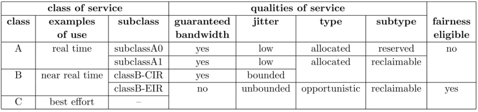
In order to meet quality of service, RPR provides three data service classes: classA (high priority), classB (medium priority), and classC (low priority). The classA service provides low-jitter transfer of traffic up to its allocated rate. Traffic above the allocated rate is rejected. The classA traffic is divided into subclassA0 and subclassA1; subclassA1 is more efficient due to reclamation. Additionally, a station’s reservation of subclassA0

2 1 N 3 5 4 6 8 N-1 N-2 7 Ringlet-0 Ringlet-1 Figure 2.1: RPR structure

bandwidth is broadcasted on the ring by using topology messages. After receiving such topology messages from all other stations on the ring, every station calculates its reservation bandwidth for subclassA0. The remaining bandwidth called unreserved rate can be used for all other traffic classes. The classB service provides bounded delay transfer of traffic at or below the committed information rate (CIR) and a best-effort transfer of the excess information rate (EIR) data beyond the committed rate. The classC service provides best-effort data-transfer services. The classC and classB-EIR are called fairness eligible (FE) traffic because such traffic is controlled by fairness algorithm. Following discussions related to fairness algorithm are all for fairness eligible traffic. These service classes are summarized in Table 2.1.

2.3

Congestion Detection and Congestion Domain

In RPR, every station transmits data as greedy as possible in order to use available bandwidth efficiently. The greedy behavior causes the total amount of transmit rate on one link to be larger than the amount of available bandwidth. The station with this overused

class of service qualities of service

class examples subclass guaranteed jitter type subtype fairness

of use bandwidth eligible

A real time subclassA0 yes low allocated reserved no

subclassA1 yes low allocated reclaimable

B near real time classB-CIR yes bounded

classB-EIR no unbounded opportunistic reclaimable yes

C best effort –

Table 2.1: Service classes and qualities of services in RPR

out-link is so-called congested. For AM and CM, the function of congestion detection is defined as IsCongested() which is triggered when STQ occupancy is over 1/8 of STQ size or all traffic except traffic of subclassA0 transmitted is larger than unreservedRate which is defined in standard and calculated by deducting reserved bandwidth from link capacity. After station detects congestion, it calculates one new local fair rate and sends one new advertised fair rate to upstream stations to suppress their traffic transiting over the congested station. IEEE802.17 standard provides one concept of congestion domain which is surrounded by head station and tail station for AM and CM. A station advertising a non-FULL RATE local fair rate is said to lie at the head of a congestion, where non-FULL RATE represents maximum of fair rate. The congestion domain extends upstream from the head station through all stations that propagate the advertised fair rate of head station until reaching a station that does not propagate the advertisement. In other words, a tail station receives an advertisement containing a non-FULL RATE fair rate but does not propagate the received fair rate further upstream. Hence, there are two simple methods to verify legal congestion domain: first, the advertised fair rate of FULL RATE does not occur in congestion domain; second, the advertised fair rate of head station is the smallest one between stations in congestion domain.

2.4

Station Structure

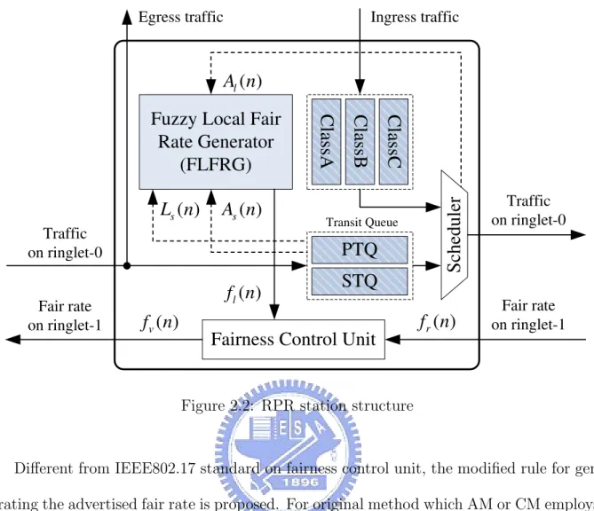
Fig. 2.2 shows the station structure related to fairness mechanism. If destination of re-ceived data is this local station, the local station strips these frames so as to pass rere-ceived frames to upper layers (i.e., egress traffic); otherwise, these received data are sent to transit queue. The transit queue buffers the data transmitting to downstream stations and the use of transit queue in ring network is so-called buffer insertion ring technology. Based on destination stripping property, the spatial reuse mechanism is realized in RPR. RPR de-fines two modes in transit queue, single queue mode and dual queue mode. Fig. 2.2 shows dual queue mode which contains the primary transit queue (PTQ) and secondary transit queue (STQ). In later discussion, the system is based on dual queue mode. When RPR uses dual queue mode, classA frames are queued in PTQ and classB and classC frames are queued in STQ, besides, PTQ, and STQ are both FIFO queues. The scheduler decides the transmitting order between add traffic (i.e., classA/classB/classC traffic added into ringlet) and transit traffic (i.e., traffic transiting PTQ and STQ) according to some rate counters. However, forwarding from PTQ has priority over STQ and most types of add traffic. FLFRG generates the local fair rate denoted as fl(n) at time nT , where T

repre-sents agingInterval, to reflect traffic condition of local station by some traffic information measured in [(n − 1)T, nT ] included arrival rate to STQ denoted as As(n), fairness eligible

traffic added into ringlet by local station denoted as Al(n), and STQ occupancy denoted as

Ls(n). The agingInterval is 100µs when link capacity is larger than or equal to 622Mbps,

otherwise, 400µs. The fairness control unit takes the received fair rate (fr(n)) sent by

downstream station and the local fair rate to generate the advertised fair rate (fv(n))

ac-cording to applied fairness algorithm. Then the advertised fair rate is sent to upstream stations to regulate upstream traffic in order to prevent bandwidth overuse.

Egress traffic Fair rate on ringlet-1 Traffic on ringlet-0

S

ch

ed

u

le

r

( )

r

f n

( )

v

f n

( )

l

f n

C

la

ss

B

C

la

ss

C

C

la

ss

A

PTQ

STQ

Fairness Control Unit

Fuzzy Local Fair

Rate Generator

(FLFRG)

Fair rate on ringlet-1 Ingress traffic Traffic on ringlet-0

( )

l

A n

( )

s

L n

A n

_s

( )

Transit Queue

Figure 2.2: RPR station structure

Different from IEEE802.17 standard on fairness control unit, the modified rule for gen-erating the advertised fair rate is proposed. For original method which AM or CM employs, one station determines whether it lies in congestion domain according to the received fair rate. If one station does not lie in congestion domain or it is the tail station of congestion domain, it sends the advertised fair rate as FULL RATE, otherwise, it sends the advertised fair rate as the smaller one between the local fair rate and the received fair rate. However, for our proposed fairness scheme, the idea of congestion domain is not such crisp, in other words, it is called “smooth” congestion domain.

In smooth congestion domain, the head station generates the smallest advertised fair rate and the received fair rate of the tail station is larger than the summation of served transit traffic transiting over the head station and add traffic transiting over the head station. The advertised fair rate is set as the smaller one between the local fair rate and

the received fair rate. However, the advertised fair rate of tail station is assigned to its local fair rate. In latter simulation, DBA and FLFRG are both based on the modified fairness control unit.

2.5

Fairness Reference Model

Fairness reference model is the goal that one fairness mechanism wants to reach. Many fairness reference models were considered like global flow-based max-min fairness, pro-portional fairness, and RIAS [5]. One of fairness reference models is RIAS proposed by Gambiroza et al. and RIAS was incorporated in IEEE802.17 draft1.0. RIAS has two key properties. The first property defines the traffic granularity for fairness at a link as an ingress-aggregated (IA) traffic flow, i.e., the aggregation of all flows originating from a given ingress station. RIAS ensures that an IA flow receives fair share of bandwidth on each link relative to other IA flows on that link. The second property of RIAS ensures maximal spatial reuse subject to first constraint. That is, bandwidth can be reclaimed by IA flows when it is unused. In other words, RIAS is a max-min fairness with traffic granularity of IA flow.

Let flow(i, j) denote the flow transmitted from source node i to destination node j. The rate of flow(i, j) is denoted as ri,j and C is the available bandwidth for fairness eligible

traffic. Without loss of generality, we assume that nodes are numbered in an increasing order with respect to direction of traffic flow, that is, for ri,j we have j > i. An IA

flow transmitted from node i and passing through link n is denoted as rn

i, where rni =

P

j>nri,j, ∀n > i. Further, let IA(i) denote the aggregation of all flows originating from

be feasible if it satisfies constraints:

rij ≥ 0, ∀j > i, (2.1a)

X

i<n

rn_i ≤ C, ∀n. (2.1b) Given a feasible rate matrix R , we say that link n is a bottleneck link with respect to

R for flow(i, j) crossing link n, and denote it by Bn(i, j), if two conditions are satisfied:

X

m

rn

m = C, rni ≥ rin0 (if rn_i0 exists) (2.2a)

rij ≥ ri0_j0, ∀j0 > n (2.2b)

A matrix of rates R is said to be RIAS fairness if it is feasible and if for each flow(i, j), rij

cannot be increased while maintaining feasibility without decreasing ri0_j0 for some f (i0, j0)

for which ri0_j0 < r_ij when i0 = i, rn i0 + rn 0 i0 ≤ r_in+ rn 0

i when rkl > 0 for l = i, i0 and k = n, n0

ri0

i0 ≤ r_ii otherwise.

(2.3) Fig. 2.3 illustrates the RIAS fair definition. Assuming that capacity is normalized and each demand of flow is infinite, the RIAS fair shares are as follows: r13 = r14 =

r15 = 20% and r12 = r25 = r45 = 40%. Consider flow(1,2), its rate cannot be increased

while maintaining feasibility without decreasing flow(1,3), flow(1,4), or flow(1,5) where

r12 ≥ r13= r14= r15. Consider flow(2,5) on bottleneck link B4(2, 5), its rate cannot be

increased while maintaining feasibility without decreasing the rate of flow(1,5) on bottleneck link B2(1, 5), where the summation of rates of IA(1) on B4(2, 5) and B2(1, 5) is equal to the

summation of rates of IA(2) on B4(2, 5) and B2(1, 5). Finally, consider flow(4,5), its rate

cannot be increased while maintaining feasibility without decreasing the rate of flow(1,5) or flow(2,5).

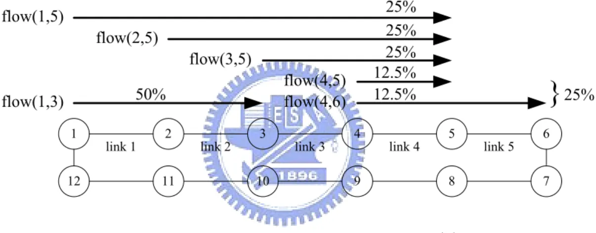
Fig. 2.4 illustrates two properties of RIAS mentioned above. Suppose that all flows have infinite demands and each flow is normalized to link capacity. For the first property

flow(1,2)

link 1 link 2 link 3 link 4

1 2 3 4 5 10 9 8 7 6 flow(1,3) flow(1,4) flow(1,5) flow(2,5) flow(4,5)

Figure 2.3: Illustration of RIAS fairness (1)

of RIAS, IA flows are shared equally that IA(1) = IA(2) = IA(3) = IA(4) = 25% on link 4, whereas node 4 divides its IA traffic among flow(4,5) and flow(4,6) equally such that flow(4,5)=flow(4,6)=12.5%. For the second property, flow(1,3) has 50% due to downstream congestion on link 4 such that flow(1,3) exploits the bandwidth on link 2. According to flow(1,3) in Fig. 2.4, RIAS ensures maximal spatial reuse. When taking RIAS as fairness reference model, what is RIAS fairness allocating given an arbitrary traffic scenario? According to [10], after assigning one legal traffic pattern, the algorithm produces one solution with regard to the given traffic scenario. Although we know the ideal RIAS fairness for arbitrary traffic pattern, there is still one challenge to implement RIAS fairness in real world RPR. DVSR [5] and DBA [6] are proposed fairness algorithms achieving RIAS fairness in real world RPR.

25% 25% 25%

{

25% 12.5% 12.5% flow(4,5) flow(1,5) flow(2,5) flow(3,5) flow(4,6) flow(1,3) 50%

link 1 link 2 link 3 link 4 link 5

1 2 3 4 5 6

12 11 10 9 8 7

Chapter 3

Fuzzy Local Fair Rate Generator

3.1

Introduction

As illustrated in Fig. 3.1, the proposed fuzzy local fair rate generator (FLFRG) is composed of fuzzy congestion detection (FCD), adaptive fair rate calculator (AFRC), and fuzzy fair rate calculator (FFRC). In order to measure congestion degree, IsCongested() is replaced by FCD such that the output of congestion detection is a fuzzy value instead of Boolean value. FLFRG takes the congestion degree into consideration in order to reflect the actual congestion situation. Because of replacing IsCongested(), the function of fairness control unit is also modified to cooperate to the proposed fairness algorithm. Based on DBA [6], AFRC generates one fair rate which estimates ideal bandwidth share of each IA flow. Then FFRC uses the fuzzy mechanism to generate the local fair rate by mainly considering the fair rate from AFRC and adjusting according to congestion degree from FCD. In Fig. 3.1, at the beginning of time nT , we denote the local fair rate by fl(n), the

output of AFRC by fd(n), and congestion degree by Dc(n). In following subsections, we

( )

c

D n

( )

s

L n

( )

s

A n

( ) l f n

( )

l

A n

Fuzzy Fair Rate

Calculator

(FFRC)

Adaptive Fair

Rate Calculator

(AFRC)

Fuzzy Congestion

Detector (FCD)

( )

d

f n

-1 z Figure 3.1: FLFRG structure

3.2

Fuzzy Logic Control System

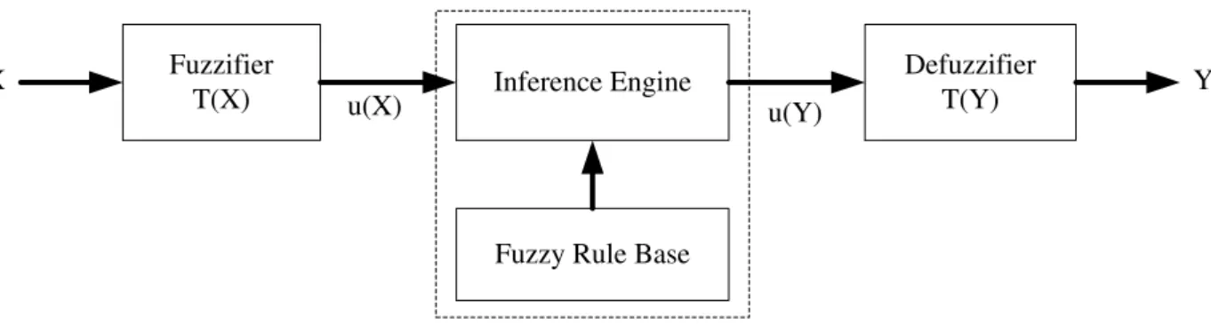
Fuzzy logic control systems have been widely applied to control nonlinear, time-varying, and ill-defined systems, in which they can provide simple and efficient solutions. A fuzzy logic controller (FLC), as shown in Fig. 3.2, has four function blocks: a fuzzifier, an inference engine, a rule base, and a defuzzifier. The fuzzifier performs the function of function of fuzzification that translates the value of each input linguistic variables X into fuzzy linguistic terms. These fuzzy linguistic terms are defined in a term set T(X) and are specified by a set of membership functions. The defuzzifier describes an output linguistic variable of the control action Y by a term set T(Y), characterized by a set of membership functions, and adopts a defuzzification strategy to convert the linguistic terms of T(Y) into a non-fuzzy value that represents control action Y. The term set should be determined at an appropriate level of granularity to describe the values of linguistic variables, and the number of terms in a term set is selected as a compromise between the complexity and the controlled performance. The fuzzy rule base is the control policy knowledge base, which is characterized be a set of linguistic statements in the form of ”if-then” rules that describe the fuzzy logic relationship between the input variables X and the control action Y. The

Fuzzifier

T(X) Inference Engine

Defuzzifier T(Y)

Fuzzy Rule Base X

u(X) _u(Y) Y

Figure 3.2: The basic structure of fuzzy logic controller

inference engine embodies the decision-making logic. It acquires the input linguistic terms of T(X) from the fuzzifier and uses an inference method to obtain the output linguistic terms of T(Y). For detail concerning the FLC, refer to [11]. The fuzzy approach can provide soft thresholds, characterize imprecise quantities, and capture a linguistic, rule-base control strategy.

3.3

Fuzzy Congestion Detector (FCD)

In IEEE802.17 standard, a station deploying dual queue mode is congested when oc-cupancy of STQ is larger than 1/8 of STQ size or all traffic except traffic of subclassA0 transmitted is larger than unreservedRate. This crisp decision of congestion detection pro-vides an explicit action for solving congestion, however, it may not reflect the actual traffic condition. For example, the urgency as occupancy of STQ equals to 2/8 of STQ size is different from the urgency as occupancy of STQ equals to 1/8 of STQ, although they are both recognized as occurrence of congestion. Here, we measure arrival rate to STQ (As(n))

and occupancy of STQ (Ls(n)) to estimate congestion condition. After measuring

conges-tion degree, it provides diversities of congesconges-tion control under different congesconges-tion degree to have a more precise decision. As shown in Fig. 3.1, As(n) and Ls(n) are the inputs of

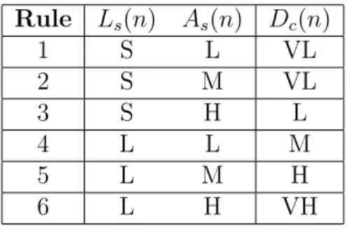
Rule Ls(n) As(n) Dc(n) 1 S L VL 2 S M VL 3 S H L 4 L L M 5 L M H 6 L H VH

Table 3.1: The rule base of FCD

congestion degree. We define the term set for As(n) as T (As(n)) = {Low (L), Medium (M),

High (H)}; for Ls(n) as T (Ls(n)) = {Short (S), Long (L)}; for Dc(n) as T (Dc(n)) = {Very

Low (VL), Low (L), Medium (M), High (H), Very High (VH)}. The rule base of FCD is shown in Table 3.1.

We use the triangular function f (x; x0, a0, a1) and the trapezoidal function g(x; x0, x1, a0, a1)

to define the membership functions for terms in the term set. These two functions are given by f (x; x0, a0, a1) =    x−x0 a0 + 1, for x0− a0 < x ≤ x0, x0−x a1 + 1, for x0 < x < x0+ a1, 0, otherwise, (3.1) and g(x; x0, x1, a0, a1) =        x−x0 a0 + 1, for x0− a0 < x ≤ x0, 1, for x0 < x ≤ x1, x1−x a1 + 1, for x1 < x < x1+ a1, 0, otherwise, (3.2)

where x0 in f(.) is the center of the triangular function; x0(x1) in g(.) is the left (right)

edge of the trapezoidal function; a0(a1) is the left (right) width of the triangular or the

trapezoidal function.

The corresponding membership functions of S and L in T (Ls(n)) are denoted as

µS(Ls(n)) = g(Ls(n); 0, 0.125Q, 0, 0.25Q), (3.3)

where Q is STQ size. Like low threshold of STQ defined in IEEE802.17 standard, 1/8 of STQ size is taken as low threshold to judge the scarce congestion. However, the high threshold we choose is a little higher than high threshold defined in IEEE802.17 standard, that is 1/4 of STQ size. When occupancy of STQ is larger than the high threshold, it indicates that urgent congestion occurs. The corresponding membership functions of L, M, and H in T (As(n)) are respectively denoted as

µL(As(n)) = g(Ls(n); 0, 0.125U, 0, 0.375U), (3.5)

µM(As(n)) = f (As(n); 0.5U, 0.25U, 0.25U), (3.6)

µH(As(n)) = g(As(n); 0.875U, U, 0.375U, 0), (3.7)

where U represents unreservedRate.

For the reason of simplicity in computation of defuzzification, let the membership func-tions for VL, L, M, H, VH in T (Dc(n)) be all fuzzy singletons and they are denoted

as µV L(Dc(n)), µL(Dc(n)), µM(Dc(n)), µH(Dc(n)), and µV H(Dc(n)), respectively. Define

these membership functions as

µV L(Dc(n)) = f (Dc(n); 0, 0, 0), (3.8)

µL(Dc(n)) = f (Dc(n); 0.25, 0, 0), (3.9)

µM(Dc(n)) = f (Dc(n); 0.5, 0, 0), (3.10)

µH(Dc(n)) = f (Dc(n); 0.75, 0, 0), (3.11)

µV H(Dc(n)) = f (Dc(n); 1, 0, 0). (3.12)

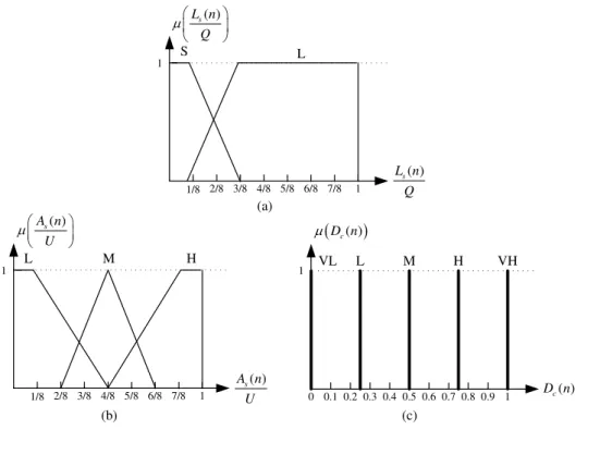
The membership functions of T (Dc(n)) distribute uniformly between 0 and 1. Fig. 3.3

1 1 VL ( ) c D n 0 0.1 0.2 0.3 0.4 0.5 0.6 0.7 0.8 0.9 L M H VH D nc( ) P (c) 1 1/8 2/8 3/8 4/8 5/8 6/8 7/8 1 L ( ) s L n Q S ( ) s L n Q P§_¨ ·_¸ © ¹ (a) ( ) s A n U 1/8 2/8 3/8 4/8 5/8 6/8 7/8 1 1 M H L ( ) s A n U P§_¨ ·_¸ © ¹ (b)

Figure 3.3: The membership functions of the term set (a) T (Ls(n)) (b) T (As(n)) (c)

T (Dc(n))

The fuzzy congestion detector adopts the max-min inference method for inference engine because it is suitable for real-time operation. To explain max-min inference method, we consider rule 1 and rule 2 which have the same control action “Dc(n) is VL”. Applying the

“min” operator, we obtain the membership function values of the control action “Dc(n) is

VL” of rule 1 and rule 2 denoted as m1(n) and m2(n) respectively, by

m1(n) = min{µS(Ls(n)), µL(As(n))}, (3.13)

m2(n) = min{µS(Ls(n)), µM(As(n))}. (3.14)

Subsequently, applying the “max” operator yields the overall membership value of the control action “Dc(n) is VL” denoted as wV L(n), by

wV L(n) = max{m1(n), m2(n)}. (3.15)

as wL(n), wM(n), wH(n), and wV H(n), respectively, can be obtained in a similar way. After

inferring all rules, the FCD uses defuzzification of center of area (COA) for defuzzifier. The output value Dc(n) is obtained as follows:

Dc(n) =

0.0 × wV L(n) + 0.25 × wL(n) + 0.5 × wM(n) + 0.75 × wH(n) + 1.0 × wV H(n)

wV L(n) + wL(n) + wM(n) + wH(n) + wV H(n)

(3.16) Therefore, Dc(n) indicates the congestion degree with a crisp value. After generating Dc(n),

FFRG takes Dc(n) as input to calculate the local fair rate.

3.4

Adaptive Fair Rate Calculator (AFRC)

As mentioned in 2.4, IEEE802.17 standard uses the local fair rate to indicate the traffic condition of local station. However, FLFRG takes the congestion degree into consideration so that a new method to estimate the local fair rate is proposed to interact with congestion degree. The first stage estimating the local fair rate is called adaptive fair rate calculator (AFRC) which algorithm is based on DBA [6]. DBA is one powerful algorithm of local fair rate generator proposed by Alharbi and Ansari and DBA, further, it is said that DBA satisfies RIAS fairness criterion. However, some constraints of DBA result in impractical realization in real world RPR. First, the local fair rate may grow to infinity, therefore, the convergence time may be large because it takes times to let fair rate go down. Second, the fair rate algorithm of DBA does not take propagation delay into account. It is possible that fair rate can not converge under varying traffic situation in large congestion domain. In order to improve these deficiencies, the fair rate algorithm of AFRC is defined as

M(n) = A˜s(n) + Al(n) fd(n − 1)

, (3.17)

fd(n) = min{C, fd(n − 1) + 1

where M(n) represents the effective number of IA flows traversing out-link of local station and is estimated in interval [(n − 1)T, nT ], ˜As(n) is the moving average version of As(n),

and C is the available fairness eligible bandwidth.

For adapting to time varying traffic conditions, a method is proposed to decide the observation interval of ˜As(n). It is composed of two parts: one is examined by flow

tran-siting over the local station with furthest source and the other is examined by hops to downstream congestion. For the former one, we assume that each station has the ability to recognize the source station of each flow and then we can get the hops count from furthest source station to local station. By checking the topology database with this hops count, we obtain the data frame trip time from furthest source station to local station, where data frame trip time is the time that the data frames traverse between two observed stations. For the latter one, each stations knows its hops to congestion and we can obtain the data frame trip time from local station to downstream congested station by checking topology database. After acquiring these two data frame trip times, station decides its observation interval of ˜As(n) by doing summation of them.

3.5

Fuzzy Fair Rate Calculator (FFRC)

As mentioned before, the local fair rate (fl(n)) affects not only fairness performance but

also bandwidth utilization. In order to generate an adaptive and robust local fair rate, we take account of the congestion degree Dc(n) and the estimated fair rate fd(n). The work of

fuzzy fair rate calculator is to generate the local fair rate in a fuzzy mechanism by mainly referring to fd(n) and adjusting according to Dc(n) Here, also define the term set for fd(n)

as T (fd(n)) ={Very Low (VL), Low (L), Slightly Low (SL), Slightly High (SH), High (H),

Very High (VH)}; for Dc(n) as T (Dc(n)) ={Low (L), Medium (M), High (H)}; for fl(n)

Rule Dc(n) fd(n) fl(n) Rule Dc(n) fd(n) fl(n) Rule Dc(n) fd(n) fl(n) 1 L V L P L 7 M V L V L 13 H V L EL 2 L L SL 8 M L L 14 H L P L 3 L SL M 9 M SL SL 15 H SL L 4 L SH H 10 M SH SH 16 H SH M 5 L H V H 11 M H P H 17 H H H 6 L V H EH 12 M V H V H 18 H V H P H

Table 3.2: The rule base of FFRC

Low (SL), Medium (M), Slightly High (SH), High (H), Pretty High (PH), Very High (VH), Extremely High (EH)}. The rule base of FFRC is shown in Table 3.2.

The membership functions of VL, L, SL, SH, H, and VH in T (fd(n)) are denoted as

µV L(fd(n)) = f (fd(n); 0, 0, 0.3U), (3.19)

µL(fd(n)) = f (fd(n); 0.2U, 0.2U, 0.2U), (3.20)

µSL(fd(n)) = f (fd(n); 0.4U, 0.2U, 0.2U), (3.21)

µSH(fd(n)) = f (fd(n); 0.6U, 0.2U, 0.2U), (3.22)

µH(fd(n)) = f (fd(n); 0.8U, 0.2U, 0.2U), (3.23)

µV H(fd(n)) = f (fd(n); U, 0.3U, 0), (3.24)

respectively, where U represents unreservedRate. These membership functions almost dis-tribute uniformly between 0 and unreservedRate. The membership functions of L, M, H in

T (Dc(n)) are respectively denoted as

µL(Dc(n)) = g(Dc(n); 0, 0.125, 0, 0.375), (3.25)

µM(Dc(n)) = f (Dc(n); 0.5, 0.25, 0.25), (3.26)

When Dc(n) is smaller than 0.5, it is viewed as “Low” congestion degree; on the contrary,

when Dc(n) is larger than 0.5, it is viewed as “High” congestion degree. Between “Low”

and “High”, “Medium” congestion degree is limited in 0.25 and 0.75. Due to simplicity of defuzzification, the membership functions of EL, VL, PL, L, SL, M, SH, H, PH, VH, and EH in T (fl(n)) are all fuzzy singletons respectively denoted as

µEL(fl(n)) = f (fl(n); 0, 0, 0), (3.28) µV L(fl(n)) = f (fl(n); 0.1U, 0, 0), (3.29) µP L(fl(n)) = f (fl(n); 0.2U, 0, 0), (3.30) µL(fl(n)) = f (fl(n); 0.3U, 0, 0), (3.31) µSL(fl(n)) = f (fl(n); 0.4U, 0, 0), (3.32) µM(fl(n)) = f (fl(n); 0.5U, 0, 0), (3.33) µSH(fl(n)) = f (fl(n); 0.6U, 0, 0), (3.34) µH(fl(n)) = f (fl(n); 0.7U, 0, 0), (3.35) µP H(fl(n)) = f (fl(n); 0.8U, 0, 0), (3.36) µV H(fl(n)) = f (fl(n); 0.9U, 0, 0), (3.37) µEH(fl(n)) = f (fl(n); U, 0, 0). (3.38)

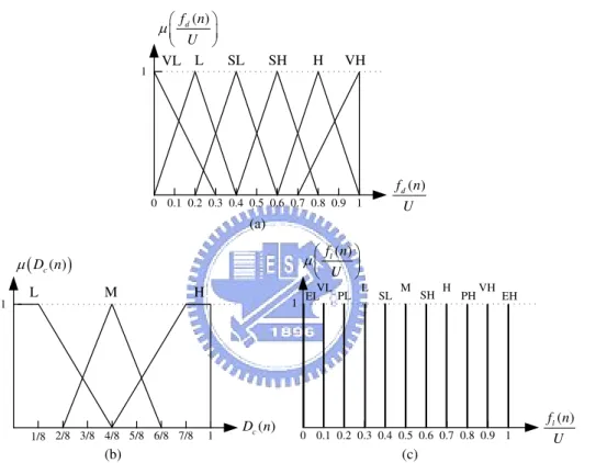
After defining the term set of local fair rate, the defuzzifier uses the method mentioned as 3.3 to generate a crisp-valued local fair rate. Eventually, a new local fair rate is sent to fairness control unit. Fig. 3.4 shows all membership functions of FFRC.

1 1/8 2/8 3/8 4/8 5/8 6/8 7/8 1 1 L M H ( ) c D n D nc( ) P (b) ( ) l f n U P §_¨ ·_¸ © ¹ 1 ( ) l f n U 0 0.1 0.2 0.3 0.4 0.5 0.6 0.7 0.8 0.9 EL (c) VL PL L SL M SH H PHVH EH 1 1 VL ( ) d f n U 0 0.1 0.2 0.3 0.4 0.5 0.6 0.7 0.8 0.9 SL SH VH ( ) d f n U P §_¨ ·_¸ © ¹ (a) L H

Figure 3.4: The membership functions of the term set (a) T (fd(n)) (b) T (Dc(n)) (c)

Chapter 4

Simulation Results and Discussions

4.1

Simulation Environment

Here, we conduct simulations to compare the performance of FLFGR with AM and DBA. The general settings of simulation environment include link capacity of 10Gbps, propagation delay between stations of 100µsec, and STQ size of 4Mbytes. The agingInterval is 100µsec and we inspect and record the simulation result per agingInterval. Assume the reserved bandwidth of classA0 is zero, in other words, the unreservedRate equals to the link capacity. Besides, only fairness eligible traffic is considered in simulations. The convergence time is obtained if the rate oscillation is in the range of 3% with respect to its ideal fair rate. Followings are scenarios set to examine the performance of fairness algorithm. Parking lot scenario with congestion domain of different size is used to observe the property of bandwidth fair share on congestion link and the influence of propagation delay. Then consider the scenario which flows start at different instants to examine the flow transient behavior and call it rate rushing scenario. Available bandwidth reclaiming scenario presents the ability of reclaiming available bandwidth. ON/OFF scenario shows the capability of rate adaptation under case of periodic time-changing demands.

4.2

Parking Lot Scenario

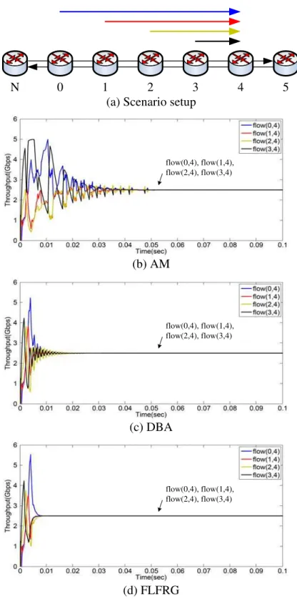
Fig. 4.1 (a) shows parking lot scenario of 5 stations and all flows in the figure are all greedy fairness eligible flows. This parking lot scenario shows that flows generate from station 0, 1, 2, 3 but terminate at the station 4. Figs. 4.1 (b), (c), and (d) present the throughput which is observed at station 4 of each flow versus time axis by AM, DBA, and FLFRG, respectively. It can be seen that after some time all flows converge to 2.5Gbps and the stability is realized for all fairness algorithms and the convergence time is about 49ms, 14ms, and 7ms by AM, DBA, and FLFRG, respectively. Consider the process of flows adaptation before accomplishing convergence by AM in Fig. 4.1 (b), in general, the maximum value of flow(3,4) decreases after every period of rate ramping up. That means the add rate of head (station 3) is getting smaller so that the advertised fair rate of head is also getting smaller because the advertised fair rate is assigned to add rate by AM as detecting congestion. When add rate of head decreases to ideal fair share rate which is 2.5Gbps in the case, head sends the advertised fair rate as 2.5Gbps to upstream station then all flows can converge after some time. Examine the rate behavior of flow(3,4) before reaching convergence in DBA in Fig. 4.1 (c), it is found that the time period of once rate ramping up and down is smaller than that of AM thus DBA has better ability of rate adaptation than AM. According to DBA, when the total rate of arrival rate to STQ and add rate is large than the available bandwidth, DBA lowers the local fair rate, otherwise raises it. Due to rate sensitivity to traffic changing, all flows can converge to the ideal fair rate more quickly than AM. See the rate behavior before achieving stability by FLFRG in Fig. 4.1 (d), flow(3,4) adapts to 2.5Gbps almost after once rate ramping up and down. It can be seen that FLFRG has outstanding performance on adapting flows to the ideal fair rate so that convergence time is much smaller than those by AM and DBA.

This is because using fuzzy logics provides a effective way to find answers by non-linear computations. According to design philosophy of FLFRG, the local fair rate is generated by the rate which is calculated by AFRC and congestion degree from FCD. FLFRG retains the good property of fast convergence coming from DBA and adjusts the local fair rate by referring to congestion degree in order to act adaptively with real traffic. When the arrival rate to STQ is too high or STQ depth excesses high threshold of STQ too much, FLFRG decreases the local fair rate to diminish congestion, otherwise raises it. In other words, FLFRG is aggressive when congestion degree is low and prudent when congestion degree is high. FLFRG generates an accurate RIAS local fair rate according to real traffic condition and non-linear computations thus FLFRG has the best performance on convergence time. Fig. 4.2 (a) shows the larger scale of parking lot scenario. AM realizes the stability and has convergence time of 23ms as shown in Fig. 4.2 (b) where only flow(0,7), flow(2,7), flow(4,7), and flow(6,7) are demonstrated due to neatness in diagram and almost the same behavior between all flows. The behavior of rate adaptation to convergence is similar to Fig. 4.1 (b) but with smaller convergence time. According to AM, after detecting disappearance of downstream congestion, stations ramps up its add rate allowed to transmit through congestion station, which is called allowedRateCongested defined in standard, with quantity proportional to the difference between link capacity and allowedRateCongested. Hence, when the difference between allowedRateCongested and link capacity is larger, station has more ability of rate adaptation. Although allowedRateCongested of each station is not shown in Fig. 4.1 (b), we take throughput of each flow as allowedRateCongested of each station because of high positive correlation between them. Compare flow(1,4) in Fig. 4.1 (b) with flow(2,7) in Fig 4.2 (b), it can be found that the difference between flow(1,4) and link capacity in Fig. 4.1 (b) is larger than the difference between flow(2,7) and link capacity in Fig 4.2 (b) at the same instant. Thus, flows converge faster in large congestion domain

(b) AM

(c) DBA

(d) FLFRG (a) Scenario setup

1 2 3 4 5 0 N flow(0,4), flow(1,4), flow(2,4), flow(3,4) flow(0,4), flow(1,4), flow(2,4), flow(3,4) flow(0,4), flow(1,4), flow(2,4), flow(3,4)

than in small congestion domain. When implementing DBA in large congestion domain, it can be found that the rate oscillation of DBA is severe at the beginning and becomes moderate as time goes by as shown in Fig. 4.2 (c). As mentioned before, DBA is sensitive to rate changing so that it performs small convergence time in small congestion domain scenario. However, the sensitivity to rate changing becomes a defect in large congestion domain. In real world, the advertised fair rate of head does not regulate all flows at one time so that the arrival rate to STQ reflects the rate which past advertised fair rate regulated. That is to say there is a time lag between current advertised fair rate and regulated arrival rate to STQ. DBA uses the information of the arrival rate to STQ to generate the local fair rate, hence an inaccuracy of the local fair rate happens and the inaccuracy becomes bigger in larger congestion domain. Moreover, the sensitivity to rate changing also enlarges the inaccuracy on the advertised fair rate. Consequently, DBA works badly in large congestion domain. Fig. 4.2 (d) considers large congestion domain by FLFRG. It performs stability and has the convergence time of 11ms which is smaller than AM. After replacing DBA by AFRC, FLFRG reduces the inaccuracy on the advertised fair rate by using moving average version of arrival rate to STQ, thus FLFRG achieves stability. Also, congestion degree is taken into consideration to indicate real traffic condition so that flows can converge to the ideal fair rate quickly.

According to the mentioned observations, AM and FLFRG both achieve stability in both scenarios but DBA only achieves it in small congestion domain. It reveals that DBA does not have the immunity against large congestion domain, in other words, the large propagation delay between head and tail in congestion domain. In small congestion domain scenario, however, DBA has better performance on convergence time than AM. As the original intention of designing FLFRG, FLFRG solves the deficiency of DBA (i.e., immunity against large congestion domain) and enhances the advantage of DBA (i.e., small

(b) AM

(c) DBA

(d) FLFRG (a) Scenario setup

flow(0,7), flow(2,7), flow(4,7)

flow(6,7) 1 2 3 4 5 0 N 6 7 8 flow(0,7), flow(2,7), flow(4,7), flow(6,7) flow(0,7), flow(2,7), flow(4,7), flow(6,7)

convergence time) then provides the best performance on stability and convergence time in both parking lot scenarios.

4.3

Rate Rushing Scenario

All flows are fairness eligible flows with demand of 4Gbps bandwidth in Fig. 4.3 (a) and flow(0,4), flow(1,4), flow(2,4), and flow(3,4) start at 0s, 0.1s, 0.2s, 0.3s, respectively. Figs. 4.3 (b), (c), and (d) present the throughput which is observed at destination station of each flow (station 4) versus time axis by AM, DBA, and FLFRG. Before 0.2s, the total demand of flow(0,4) and flow(1,4) is 8Gbps which is under link capacity 10Gbps so flows are unobstructed. After 0.2s, the join of flow(2,4) makes the congestion occur at station 2. Fig. 4.3 (b) shows the behavior of flows by using AM. Observe behavior of flows in [0.2s, 0.3s]. It is found that flow(0,4) has larger throughput than flow(1,4) in general in [0.2s, 0.22s]. The reasons are that station 1 does not sends the advertised fair rate which is generated from congested station 2 to station 0 thus station 0 is not conscious of downstream congestion at most time, however, station 1 detects downstream congestion of station 2. For this reason, flow(0,4) is not throttled but flow(1,4) is. After about 61ms, station 1 detects downstream congestion and suppresses its add rate then all flows converge to the ideal fair rate. Observe behavior of flows in [0.3s, 0.5s]. Flow(0,4), flow(1,4), and flow(2,4) are throttled in a short time after join of flow(3,4) at 0.3s, hence, flows converge to ideal fair rate in [0.3s, 0.5s] with the convergence time of 18ms which is much smaller than it in [0.2s, 0.3s]. Fig. 4.3 (c) shows the simulation result by using DBA. It can be found that at the transient of 0.2s and 0.3s, the convergence time are about 3ms and 12ms, respectively, which are both much smaller than in Fig. 4.3 (b). The reasons are that, first, a precise local fair rate is generated by DBA in small congestion domain; second, since the function of fairness control unit is modified as description in 2.4, the advertised fair rate of head station could be arrived at

station 0 factually not like AM does. Fig. 4.3 (d) shows the simulation result by using FLFRG. At the transient of 0.2s, Fig. 4.3 (d) demonstrates a convergence time of 5ms. At the transient of 0.3s, the convergence time in Fig. 4.3 (d) is about 4ms which is much smaller than convergence time in Fig. 4.3 (b) and (c). Recall the function block of FCD in FLFRG, the STQ occupancy is used to measure congestion degree, where STQ occupancy plays a significant role. STQ occupancy mainly reflects the consequence of congestion, in other words, when one station is heavily congested, its STQ occupancy must be very high. By applying FCD, the congestion degree is measured to reveal actual congestion condition. The application of congestion degree makes FLFRG more adaptive than DBA so that flows converge faster by FLFRG than by DBA.

4.4

Available Bandwidth Reclaiming Scenario

Consider the scenario illustrated in Fig. 4.4 (a), where all flows are greedy fairness eligible flows and start at 0s. In order to keep the simulation result clear and neat, we do not show all flows but only demonstrate the behaviors of flow(0,3), flow(1,8), flow(2,8), flow(4,8), and flow(7,8), besides, all flows except flow(0,3) act in a similar way. Fig. 4.4 (b) shows the simulation result of AM. After some time, due to congestion experienced at link 2 which is out-link of station 2, station 2 sends its fair rate to station 0 to suppress flow(0,3). Station 0 perceives cease of downstream congestion when receiving FULL RATE, then raises its add rate to reclaim available bandwidth till congestion happens again. According to AM, the advertised fair rate of the head in congestion domain is assigned to its add rate such that it is possible to send a small fair rate to over-throttle flows like flow(0,3) which oscillates in range between about 3Gbps and 7.4Gbps.

Fig. 4.4 (c) shows the simulation result of DBA. Compared with AM, flow(0,3) is more stable than by AM but flow(2,8) oscillates severely. It is because station 2 is the

(b) AM (c) DBA (d) FLFRG 1 2 3 4 5 0 N

(a) Scenario setup

(b) AM

(c) DBA

(d) FLFRG (a) Scenario setup

1 2 3 4 5

0

N 6 7 8 9

flow(1,8), flow(2,8),

flow(4,8), flow(7,8) flow(0,3)

flow(1,8), flow(2,8), flow(4,8), flow(7,8) flow(0,3) flow(1,8), flow(2,8), flow(4,8), flow(7,8) flow(0,3)

conjunction between two congestion domains which heads are station 2 and station 7, such that congestion state of station 2 changes frequently so that the local fair rate is fluctuated. Like the reasons mentioned before, flows fluctuate gravely by using DBA when the advertised fair rate do not regulate upstream flows immediately. Moreover, the add rate of station 2 also be affected by the received fair rate from downstream congested station (station 7), hence, it is harder to generate a stable local fair rate. Unlike Fig. 4.4 (c), Figs. 4.4 (d) shows a more stable behavior of flows by FLFRG. The reasons are that FLFRG consider the congestion degree and diminishes the vibration of arrival rates to STQ then generates an appropriate local fair rate. When we consider the average value of all flows, Figs. 4.4 (c) and (d) show that flows satisfy RIAS fairness in some sense (flow(0,3) shares 7143Mbps; other flows share 1429Mbps), however, the rate oscillation is smaller by FLFRG than by DBA.

4.5

ON/OFF Scenario

In this simulation, as shown in Fig. 4.5 (a), flow(0,5) is an ON/OFF fairness eligible flow with period of 0.1s and it demands 1Gbps at ON state. Flow(3,5) and flow(4,5) are both greedy fairness eligible flows and start at 0.1s and 0.2s, respectively. See the simulation result of AM in Fig 4.5 (b), as observing in [0.1s 0.2s], flow(0,3) shares bandwidth of 9Gbps when flow(0,5) is at ON state and then grows to 10Gbps when flow(0,5) turns to OFF state. At the transient of 0.2s, station 4 detects congestion and then sends the advertised fair rate to suppress flow(0,5) and flow(3,5). After solving congestion, station 4 raises its add rate until congestion occurs again. Flow(4,5) reaches its peak value of 6.5Gbps then decreases to 5Gbps in [0.2s 0.23s] as shown in Fig 4.5 (b). The value of 5Gbps comes from bandwidth equally share between add traffic and transit traffic under specific traffic condition according to AM. After some time, flow(4,5) and flow(3,5) converge to

(b) (c) (d) (a) 1 2 3 4 5 0 N 6 flow(0,5) flow(3,5), flow(4,5) flow(0,5) flow(3,5), flow(4,5) flow(0,5) flow(3,5), flow(4,5)

the ideal fair rate 4.5Gbps. In general, flow(3,5) and flow(4,5) do not converge to 4.5Gbps immediately after each ON/OFF transient of flow(0,5). See Fig. 4.5 (c) and (d) by using DBA and FLFRG respectively, the severe oscillation does not happen and flows converge to the ideal fair rate very fast. An excellent performance on convergence time be realized both by DBA and FLFRG.

Chapter 5

Conclusions

In this thesis, the fairness issue in RPR when congestion occurs is studied. The fairness algorithm named FLFRG is proposed to guarantee stability, satisfy fairness criterion as RIAS fairness, and make flows converge to the ideal fair rate quickly. It is clear to under-stand that if more information are used to make a decision then the decision would be more precise. By implementing fuzzy logic control system, FLFRG adopts information from add rate, transit rate, and STQ occupancy to generate a precise local fair rate.

FLFRG is composed of three function block which are AFRC, FCD, and FFRC. AFRC generates an estimated fair rate by modifying DBA, thus it has immunity against large propagation delay. FCD produces a congestion degree to indicate the urgency of congestion instead of whether congestion occurs. After adopting the two terms from AFRC and FCD, FFRC generates one local fair rate by fuzzy logics. Because of applying congestion degree, FLFRG generates the local fair rate aggressively when the congestion is slight and cautiously when the congestion is heavy. That is to say that FLFRG takes smart and fast action against the changing traffic conditions.

Fairness algorithms like AM, DBA, and FLFRG are applied in different scenarios to see their performance on stability and convergence time. Generally speaking, AM reaches stability in most scenarios but has large convergence time; DBA achieves stability only

in small scale of congestion domain due to the influence of propagation delay, however, DBA has smaller convergence time than AM if stability is realized. Unlike DBA which stability is only attained in specific environment, FLFRG overcomes the constraints of large scale of congestion domain then achieves stability, moreover, FLFRG also considers congestion degree to adjust the local fair rate so that the ability of adaption to ideal fair rate is enhanced. Besides, FLFRG always satisfy RIAS fairness in all test scenarios. It is concluded that FLFRG has the excellent performance on stability, fairness, and convergence time.

Bibliography

[1] IEEE Standard 802.17, “Resilient Packet Ring (RPR) Access Method and Physical Layer Specification,” 2004.

[2] F. Davik, M. Yilmaz, S. Gjessing, and N. Uzun, “IEEE 802.17 Resilient Packet Ring Tutorial,” IEEE Commun. Mag., vol. 42, no. 3, pp. 112 - 118, March 2004.

[3] A. Shokrani, J. Talim, and I. Lambadaris, “Modeling and Analysis of Fair Rate Cal-culation in Resilient Packet Ring Conservative Mode,” IEEE ICC 2006 proceedings, vol.1, pp. 203 - 210, June 2006.

[4] F. Davik, A. Kvalbein, and S. Gjessing, “An Analytical Bound for Convergence of the Resilient Packet Ring Aggressive Mode Fairness Algorithm,” IEEE ICC 2005

proceed-ings, vol. 1, pp.281 - 287, May 2005.

[5] V. Gambiroza, P. Yuan, L. Balzano, Y. Liu, S. Sheafor, and E. Knightly, “Design, analysis, and implementation of DVSR: a fair high-performance protocol for packet rings,” IEEE/ACM Trans. Networking, vol. 12, no. 1, pp. 85 - 102, February 2004. [6] F. Alharbi and N. Ansari, “Distributed bandwidth allocation for resilient packet ring

networks,” Computer Networks, vol.49, no. 2, pp.161 - 171, October 2005.

[7] F. Alharbi and N. Ansari, “SSA: simple scheduling algorithm for resilient packet ring networks,” IEE Proceedings Communications, vol.153, no. 2, pp.183 - 188, April 2006. [8] F. Davik, A. Kvalbein, and S. Gjessing, “Congestion Domain Boundaries in Resilient

Packet Rings,” Tech. Rep., Simula Research Laboratory, February 2005.

[9] M. Yilmaz and N. Ansari, “Weighted Fairness in Resilient Packet Rings,” IEEE ICC

2007, June 2007.

[10] RIAS matlab code. http://www.ece.rice.edu/networks/RIAS/

[11] Chin-Teng Lin and C.S. George Lee, “Neural Fuzzy Systems: A Neuro-Fuzzy Syner-gism to Intelligent Systems,” Prentice Hall, 1995.

[12] A. Thombare and Y. Viniotis, “Resilient Packet Ring: Bandwidth Reclamation and STQ Size Requirements,” CSNDSP 2006, July 2006.

Vita

Wei-Chien Wang was born in Pingtung, Taiwan. He received B.E. degree in Depart-ment of Communication Engineering and M.E. degree in DepartDepart-ment of Communication Engineering from Nation Chiao-Tung University, Hsinchu, Taiwan, in 2006 and 2008, re-spectively. His research interests include resilient packet ring, resource management, and intelligent techniques involving fuzzy logic.