廣義財務模型於保險公司資產配置與破產成本之研究 - 政大學術集成

全文

(1)國立政治大學風險管理與保險學系博士論文指導教授：張士傑博士. 政治大. 立廣義財務模型於保險公司資產配置與破產成本之研究. ‧ 國. 學. Asset Allocation and Bankruptcy Problems of Insurance. ‧. Company in General Financial Models. n. er. io. sit. y. Nat. al. Ch. engchi. i n U. v. 博士生：楊尚穎中華民國一○○年六月.

(2) Contests Abstract ..................................................................................................................... 1 Chapter 1 Introduction ............................................................................................... 3 Chapter 2 Exchange Rate Predictability in International Portfolio Selection .............. 8 2.1. Introduction........................................................................................ 8 2.2. The Market Framework and the Model............................................. 14 2.3. Learning Process .............................................................................. 18 2.4. The Martingale Method .................................................................... 23 2.5. The Optimization Program ............................................................... 24 2.6. A Simplified Example Revisited ....................................................... 28 2.7. Numerical illustration ....................................................................... 38 2.8. Conclusion ....................................................................................... 54 Chapter 3 Too Big to Fail or Too Small to Save: Regulatory Forbearance and Guarantee Benefits in Taiwan’s Life Insurance Market............................................ 57 3.1. Introduction...................................................................................... 57 3.2. Contract specification and Guarantee Benefit Index ......................... 62 3.2.1. Contract specification ............................................................... 62 3.2.2. Market environment ................................................................. 65 3.2.3. Quantitative index of regulatory forbearance ............................ 67 3.3. Relative and Absolute intervention criterion ..................................... 71 3.4. Numerical analysis ........................................................................... 76 3.4.3. Scenario analysis ...................................................................... 79 3.4.3.1. The effects of riskless interest rate and minimal guarantee interest rate....................................................................................... 79 3.4.3.2. The effect of asset volatility .............................................. 81 3.4.3.3. The effect of different intervention criterion...................... 82 3.5. Conclusion ....................................................................................... 83 Chapter 4 An Analysis of the Bankruptcy Cost of Insurance Guaranty Fund under Regulatory Forbearance ........................................................................................... 85 4.1. Introduction and Motivation ............................................................. 85 4.1.1. Legacy Issues ........................................................................... 88 4.1.2. Government Intervention and Forbearance ............................... 89 4.1.3. Literature Review of Bankruptcy Problem ................................ 90 4.2. The Model........................................................................................ 95 4.2.1. Market Framework ................................................................... 95 4.2.2. Cost of Insurance Guaranty Fund .............................................. 98 4.3. Numerical analysis ..........................................................................103. 立. 政治大. ‧. ‧ 國. 學. n. er. io. sit. y. Nat. al. Ch. engchi. ii. i n U. v.

(3) 4.4. Conclusion ...................................................................................... 117 Appendix A ............................................................................................................ 119 Appendix A.1 ................................................................................................. 119 Appendix A.2 Parameter values used in numerical analysis ............................122 Appendix A.3 Glossary of the notations ..........................................................124 Appendix B ............................................................................................................126 Appendix C: cost of bankruptcy of Guaranty fund ..................................................131 Reference ...............................................................................................................133. 立. 政治大. ‧. ‧ 國. 學. n. er. io. sit. y. Nat. al. Ch. engchi. iii. i n U. v.

(4) List of Tables Table 2.1 Outperform benchmark based on the exchange rate processes .................. 40 Table 2.2 Mean return of exchange rate with and without learning ........................... 41 Table 3.1 Balance Sheet of Insurance Company....................................................... 62 Table 3.2 The guarantee benefit index M(0) with parameter: A0 = 100; L0 = 95; α = 0.95; r = 0.02; g = 0.015; σ = 0.05。 ...................................................... 78. Table 3.3 The guarantee benefit index of the condition r = 𝑔 with parameters: A0 = 100; L0 = 95; α = 0.95; r = 0.02; g = 0.02; σ = 0.05 ................................. 80 Table 3.4 The guarantee benefit index of the condition r < 𝑔 with parameters: A0 = 100; L0 = 95; α = 0.95; r = 0.015; g = 0.02; σ = 0.05 ............................... 80 Table 3.5 The guarantee benefit index M(0) with parameter: A0 = 100; L0 = 95; α = 0.95; r = 0.02; g = 0.015; σ = 0.1。 ........................................................ 81. ‧ 國. 學. 政治大 Table 3.6 The guarantee benefit index M(0) with parameter: A0 = 100; L0 = 立 95; α = 0.95; r = 0.02; g = 0.015; σ = 0.15。 ...................................................... 82 Table 3.7 The average force of regulatory in difference intervention criterions with. ‧. parameters: α = 0.95; r = 0.02; g = 0.015; σ = 0.05; η = 0.9; Υ = 50 ................. 83 Table 4.1 Balance Sheet of Insurance Company....................................................... 95 Table 4.2 The bankruptcy cost per liability value with parameters: ......................... 113 α = 0.95(leverage ratio); r = 2%(risk free interest rate); g = 1.5%(minimal guarantee rate); η = 100%(monitoring ratio) ..................... 113. sit. y. Nat. n. al. er. io. Table 4.3 The bankruptcy cost per liability value with parameters: ......................... 113 α = 0.9(leverage ratio); r = 2%(risk free interest rate); g = 1.5%(minimal guarantee rate); η = 100%(monitoring ratio) .................... 113. Ch. engchi. i n U. v. Table 4.4 The bankruptcy cost per liability value with parameters: ......................... 114 α = 0.85(leverage ratio); r = 2%(risk free interest rate); g = 1.5%(minimal guarantee rate); η = 100%(monitoring ratio) .................... 114. Table 4.5 The bankruptcy cost per liability value with parameters: ......................... 114 α = 0.95(leverage ratio); r = 2%(risk free interest rate); g = 1.5%(minimal guarantee rate); η = 90%(monitoring ratio) ....................... 114 Table 4.6 The bankruptcy cost per liability value with parameters: ......................... 115 α = 0.9(leverage ratio); r = 2%(risk free interest rate); g = 1.5%(minimal guarantee rate); η = 90%(monitoring ratio) ....................... 115 Table 4.7 The bankruptcy cost per liability value with parameters: ......................... 115 α = 0.85(leverage ratio); r = 2%(risk free interest rate); g = 1.5%(minimal guarantee rate); η = 90%(monitoring ratio) ...................... 115 Table 4.8 The bankruptcy cost per liability value with parameters: ......................... 116 iv.

(5) α = 0.95(leverage ratio); r = 2%(risk free interest rate); g = 1.5%(minimal guarantee rate); η = 80%(monitoring ratio) ...................... 116 Table 4.9 The bankruptcy cost per liability value with parameters: ......................... 116 α = 0.9(leverage ratio); r = 2%(risk free interest rate); g = 1.5%(minimal guarantee rate); η = 80%(monitoring ratio) ....................... 116 Table 4.10 The bankruptcy cost per liability value with parameters: ....................... 117 α = 0.85(leverage ratio); r = 2%(risk free interest rate); g = 1.5%(minimal guarantee rate); η = 80%(monitoring ratio) ....................... 117. 立. 政治大. ‧. ‧ 國. 學. n. er. io. sit. y. Nat. al. Ch. engchi. v. i n U. v.

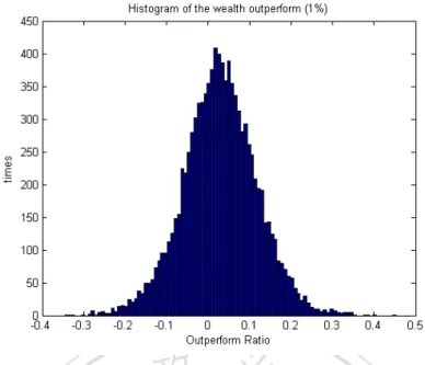
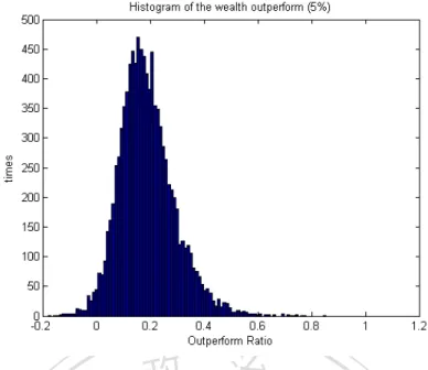
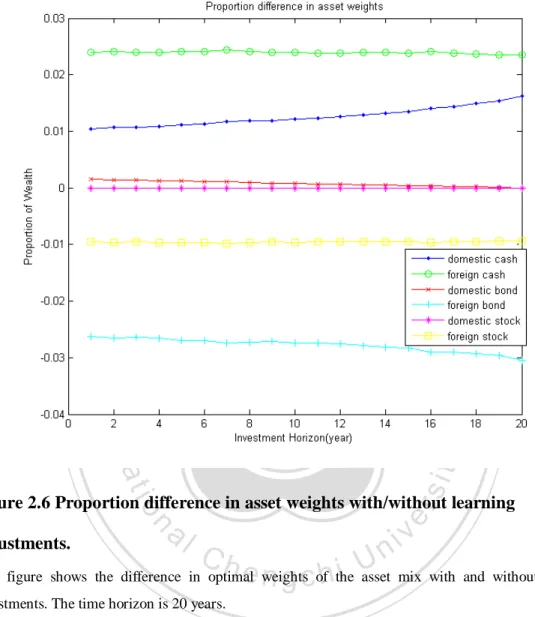
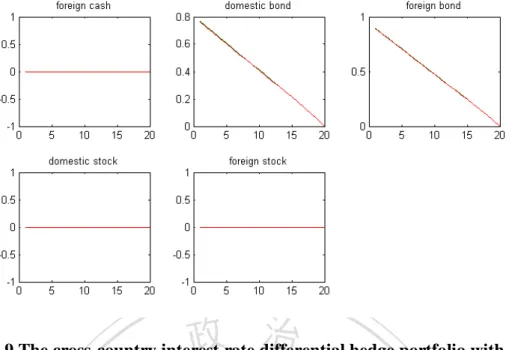
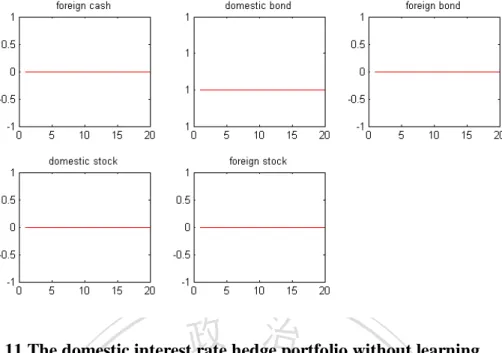
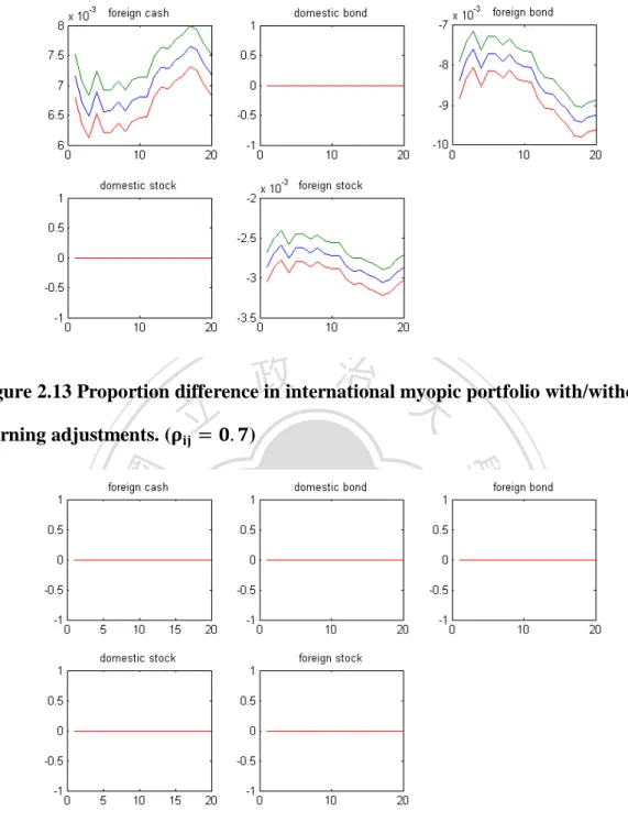
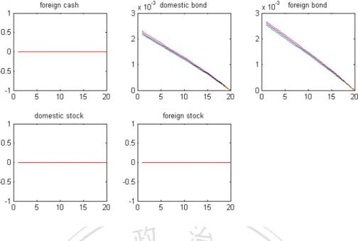
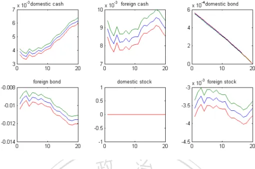
(6) List of Figures. Figure 2.1 Histogram of the terminal wealth given mean return of the exchange rate process 1%. ............................................................................................................. 39 Figure 2.2 Histogram of the terminal wealth given mean return of the exchange rate process 3% .............................................................................................................. 39 Figure 2.3 Histogram of the terminal wealth given mean return of the exchange rate process 5% .............................................................................................................. 40 Figure 2.4 Asset allocation with learning adjustments .............................................. 42 Figure 2.5 Asset allocation without learning adjustments ......................................... 42 Figure 2.6 Proportion difference in asset weights with/without learning adjustments. ................................................................................................................................ 43. ‧ 國. 學. 政治大 Figure 2.7 The international myopic portfolio with learning adjustments. (ρij = 0.7) 立 ................................................................................................................................ 44 Figure 2.8 The domestic interest rate hedge portfolio with learning adjustments.. ‧. (ρij = 0.7) ............................................................................................................... 44 Figure 2.9 The cross-country interest rate differential hedge portfolio with learning. y. Nat. adjustments. (ρij = 0.7)........................................................................................... 45 Figure 2.10 The international myopic portfolio without learning adjustments.. sit. er. io. (ρij = 0.7) ............................................................................................................... 45 Figure 2.11 The domestic interest rate hedge portfolio without learning adjustments. (ρij = 0.7) ............................................................................................................... 46 Figure 2.12 The cross-country interest rate differential hedge portfolio without. n. al. Ch. engchi. i n U. v. learning adjustments. (ρij = 0.7) ............................................................................. 46 Figure 2.13 Proportion difference in international myopic portfolio with/without learning adjustments. (ρij = 0.7) ............................................................................. 47 Figure 2.14 Proportion difference in domestic interest rate hedge portfolio with/without learning adjustments. (ρij = 0.7) ........................................................ 47 Figure 2.15 Proportion difference in cross-country interest rate differential hedge portfolio with/without learning adjustments. (ρij = 0.7) .......................................... 48 Figure 2.16 Asset allocation with learning adjustments (ρij = 0.7 and γ = 0.2) ..... 49 Figure 2.17 Asset allocation without learning adjustments (ρij = 0.7 and γ = 0.2) 49 Figure 2.18 Proportion difference in asset weights with/without learning adjustments.. (ρij = 0.7 and γ = 0.2).......................................................................................... 50 Figure 2.19 Asset allocation with learning adjustments (ρij = 0.7 and γ = 0.5) ..... 50 Figure 2.20 Asset allocation without learning adjustments (ρij = 0.7 and γ = 0.5) 51 vi.

(7) Figure 2.21 Proportion difference in asset weights with/without learning adjustments. (ρij = 0.7 and γ = 0.5).......................................................................................... 51 Figure 2.22 Asset allocation with learning adjustments (ρij = 0.7 and γ = 0.8) ..... 52 Figure 2.23 Asset allocation without learning adjustments (ρij = 0.7 and γ = 0.8) 52 Figure 2.24 Proportion difference in asset weights with/without learning adjustments.. (ρij = 0.7 and γ = 0.8).......................................................................................... 53 Figure 2.25 The conditional variance estimates over the time horizon. ..................... 54 Figure 3.1 The payoff to the policyholder at maturity .............................................. 63 Figure 3.2 Relationship between A0 and average regulatory intensity MR0A0：blue, MA0A0：red, with parameters α = 0.95; r = 0.02; g = 0.015; d = 0.5; η = 0.9; Υ =. 50; T = 20; σ = 0.1 ................................................................................................ 75 Figure 4.1 Cost of the guaranty fund given different leverage ratios and grace periods if default happened after maturity ...........................................................................103 Figure 4.2 Cost of the guaranty fund given different leverage ratios and grace periods if default happened before maturity ........................................................................104 Figure 4.3 The total cost of the guaranty fund given different leverage ratios and grace periods ...................................................................................................................104 Figure 4.4 The total cost of the guaranty fund per liability given different leverage ratios and grace periods ..........................................................................................105 Figure 4.5 Cost of the guaranty fund given different ratios of monitoring and grace periods if default happened after maturity ...............................................................106 Figure 4.6 Cost of the guaranty fund given different ratios of monitoring and grace periods if default happened before maturity ............................................................107 Figure 4.7 The total cost of the guaranty fund with different given different ratios of monitoring and grace periods..................................................................................107 Figure 4.8 The total cost of the guaranty fund per liability given different ratios of monitoring and grace periods..................................................................................108 Figure 4.9 Cost of the guaranty fund given different volatilities and grace periods if default happened after maturity ..............................................................................109 Figure 4.10 Cost of the guaranty fund given different volatilities and grace periods if default happened before maturity............................................................................ 110 Figure 4.11 The total cost of the guaranty fund given different volatilities and grace periods ................................................................................................................... 110 Figure 4.12 The total cost of the guaranty fund per liability given different volatilities and grace periods.................................................................................................... 111. 立. 政治大. ‧. ‧ 國. 學. n. er. io. sit. y. Nat. al. Ch. engchi. vii. i n U. v.

(8) Abstract This thesis focuses on the international portfolio selection and the bankruptcy cost of the insurance company under regulatory forbearance. The main theme of this thesis is outlined in chapter 1, which also serves as an introduction to the three papers (appearing here as Chapter 2, Chapter 3 and Chapter 4) collected in this thesis. In the theme of the international portfolio selection, Chapter 2 investigates the investment behaviors when learning effect is considered. According to the exchange. 政治大. rate predictability, the investor updates his information and adjusts his portfolio. 立. allocation. Finally, the numerical results show that the learning mechanism. ‧ 國. 學. significantly improves the terminal wealth.. In the theme of the regulatory forbearance, Chapter 3 provides an illustration of. ‧. the impact on the ruin cost due to regulatory forbearance. The concept of the U.S.. y. Nat. io. sit. Chapter 11 bankruptcy code is employed to determine regulatory forbearance.. n. al. er. Throughout the framework of Parisian option, a quantitative index of regulatory. i n U. v. forbearance called Guarantee Benefit Index (GBI) is developed. The GBI is used to. Ch. engchi. evaluate the different supervisory intervention criteria i.e., relative and absolute intervention criteria. Finally, numerical analysis is performed to illustrate the influence of different financial factors and the intervention criteria. Another important issue in bankruptcy problem is discussed in Chapter 4, i.e., the cost of insurance guaranty fund. It is important to determine the cost of bankruptcy when the insolvent insurance company is took over by the government. Under the U.S. Chapter 11 bankruptcy code, the cost of guaranty fund can be determined through Parisian options. Results show that the current premium rates of Taiwan insurance guarantee fund are far from risk sensitive. Hence the results suggest 1.

(9) the government should more prudent to face the bankruptcy problem in insurance industry.. 立. 政治大. ‧. ‧ 國. 學. n. er. io. sit. y. Nat. al. Ch. engchi. 2. i n U. v.

(10) Chapter 1 Introduction This thesis aims to investigate two important issues for long term investors, i.e., solving the optimal asset allocation allowing international investment and evaluating the cost of bankruptcy considering regulatory forbearance. According to portfolio choice theory in Solnik (1974) and Grauer and Hakansson (1987), economists have long been conscious of the advantage of global diversification. However, the role of the exchange rate affection is not well evaluated. 政治大 well-documented phenomenon 立 (see, e.g., Mark (1995), Allen and Taylor (1992), and. in literatures. The empirical results on long-term predictability of exchange rates are a. ‧ 國. 學. Kilian and Taylor (2003)). Therefore, the learning effect of exchange rate prediction is incorporated to solving the international asset allocation in chapter 2.. ‧. The bankruptcy announced by Lehman brother which cause the global financial. sit. y. Nat. crisis of 2008. The major center bank around the world cut the interest rate in the. n. al. er. io. coordinate move and its lead the global economy into an unprecedented low interest. i n U. v. environment. Negative interest rate has been an urgent situation in Taiwanese life. Ch. engchi. insurance industry and become worse due to the action from the major center bank. Several Taiwan life insurance company are facing large assets depreciation and insolvency problem accord to the risk-based capital (RBC) requirement. To relieve the domestic life insurer solvency capital pressure, the Financial Supervisory Commission (FSC) relaxed the RBC requirements to slow down the fall in insurer RBC resulting from the depression in the domestic stock market. However, Kuo Hua Life Insurance had been took control by the FSC on August 5 2009. As the end of December 2009, Kuo Hao had a negative net worth of NT$62.1 billion, with assets valued at NT$256 billion and 2 million policyholders. Due to the large loss in the life insurance industry, 3.

(11) solvency and capital adequacy problems is critical for existing life insurers and for potential new entrants to the market. When the company faces the insolvent problem, the regulator might adopt the action of regulatory forbearance to delay its bankruptcy, which means a regulator reduce the scope of regulation or withdraw entirely from regulating specified markets. Hence, in the study two questions are explored when the regulator adopting the regulatory forbearance approach. There are “How to define a quantitative index of regulatory forbearance to evaluate the different government intervention criteria” which is discussed in chapter 3, and “How to examine the cost. 政治大. of insurance guaranty fund incorporating the regulatory forbearance” is illustrated in chapter 4.. 立. Chapter 2, entitled “Exchange Rate Predictability in International Portfolio. ‧ 國. 學. Selection”, provides theoretical findings and the numerical illustrations of exchange. ‧. rate predictability in the international portfolio choice problem. Uncertainty regarding. sit. y. Nat. the predictive relation affects the optimal portfolio selection through dynamic learning,. io. er. and creates a state-dependent relation between the optimal asset allocation and the investment time horizon. This study investigates the investment behaviors of constant. al. n. v i n C h and adjusts the relative risk adverse (CRRA) investors exchange rate process by the engchi U observed interest rate dynamics. This approach is implemented through a filtering mechanism to evaluate the learning effects in the portfolio selection problem that. were not fully explored by Lioui and Poncet (2003). Since the learning process updates the market price of exchange rate risk, this approach makes the necessary modifications based on exchange rate predictability. This study presents numerical illustrations showing that the learning mechanism significantly increases the terminal wealth, and investigates the effect of learning on the asset mix. We find that: 1. The optimal portfolio selection can be depicted through the four-fund theorem introduced by Rudolf and Ziemba (2004). The four funds are the international 4.

(12) myopic portfolio, the domestic interest rate hedge portfolio, the cross-country interest rate differential hedge portfolio, and the domestic riskless asset. The proportions of each fund invested in the individual assets depend only on the asset return characteristics and not on investor preferences; and the investor’s optimal demands for the three funds depend on his preferences. 2. The learning effect enhances the terminal wealth performance for strategic investors. However, the improvement ratio decreases with declining the mean return of the exchange rate.. 政治大 Forbearance and Guarantee Benefits in Taiwan Life Insurance Market”, provides 立. Chapter 3, entitled “Too Big to Fail or Too Small to Save: Regulatory. illustration of the definition of regulatory forbearance in academic. The global. ‧ 國. 學. financial crisis in 2008 resulted in systematic risks in the equity, asset, and credit. ‧. markets that created significant deprecation in the life insurer’s balance sheet. To. sit. y. Nat. maintain prudent supervision and market stability, supervisory bodies announced a. io. er. temporary risk-based capital relief plan. Hence, maintaining solvency standard became a critical issue to avoid moral hazard for the market players and potential. al. n. v i n C h based on aUprudent regulation framework. entrants, forcing them to be competent engchi. Following Grosen and Jogensen (2002) and Chen and Suchanecki (2007), this study explicitly calculates the guarantee benefits based on the financial leverage of the insurer and plausible regulatory forbearance through a Parisian barrier option. This study compares relative and absolute intervention criteria by measuring theirs effect on the guarantees benefits. Results show that the relative intervention criterion is more sensitive to financial leverage than the absolute intervention criterion is. Thus, increasing the leverage ratio of the insurer increases the guarantee benefit per asset. Conversely, extending the relief plan and reducing the intervention standard decreases guarantee benefit per asset. These effects decrease if the forbearance 5.

(13) duration or the minimal intervention standards exceed certain levels. We show that: 1. The guarantee benefit index can capture the two features about regulatory forbearance. As the change of grace period and the change of the ratio of monitoring, the guarantee benefit index reflects the variation sensitivity. 2. Comparing different intervention criteria, relative intervention criterion results a uniform force of regulatory with respect to different firm sizes. If the grace period is longer enough, the average force of regulatory of two different intervention criteria will converge to a steady state.. 政治大 Fund under Regulatory Forbearance”, provides an analytical treatment for the cost of 立. Chapter 4, entitled “An Analysis of the Bankruptcy Cost of Insurance Guaranty. guaranty fund. This study investigates the bankruptcy cost when a financially. ‧ 國. 學. distressed life insurer is taken over by the supervision authority. Specifically, this. ‧. study adopts the framework proposed in Grosen and Jogensen (2002) and Chen and. sit. y. Nat. Suchanecki (2007) to measure the implied default cost of the Taiwan insurance. io. er. guaranty fund (TIGF) during the financial restructuring. The compensation of the guaranty fund is calculated incorporating the grace periods caused by the regulatory. al. n. v i n forbearance, which is similar toCChapter 11 bankruptcy h e n g c h i U procedures in the US Code.. This study adds to the previous works of Cummins (1988) and Duan and Yu (2005) by explicitly defining the embedded default options and incorporating the grace period induced by the regulatory forbearance. The main results are: 1. Beside some special condition, the leverage ratio, asset volatility, and the ratio of monitoring have the parallel effect to the cost of guaranty fund. Asset volatility is the most important factor affected the bankruptcy cost while the financial ratio and intervention criterion have shown relatively minor influence. 2. The current premium rates (i.e., 20 basis points for non-life insurers and 10 basis points for life insurers) for the Taiwan insurance guaranty fund are not risk 6.

(14) sensitive and hence the financial restructuring should be designed to ease the moral hazard problem. The above three essays study two research topic about portfolio selection and bankruptcy. In current life insurance industry, cross-country investment is conversant with insurance company. We exploit the learning mechanism to improve the terminal wealth which has significant effect. After global financial crisis, the life insurance industry had suffered asset value shirked by the fluctuated capital market. How to reduce the bankruptcy cost through early regulatory intervention becomes an. 政治大 called the guarantee benefit index to evaluate the force of regulatory and price the cost 立. important public issue. We construct a quantitative index of regulatory forbearance. of guaranty fund.. ‧ 國. 學. This thesis proceeds as follows: Chapter 2 investigates international asset. ‧. allocation incorporating the exchange rate prediction. Chapter 3 evaluates a. sit. y. Nat. benchmark index of regulatory forbearance and uses this index to compare different. io. al. n. 4.. er. intervention criteria. The cost of guaranty fund is priced under regulatory in Chapter. Ch. engchi. 7. i n U. v.

(15) Chapter 2 Exchange Rate Predictability in International Portfolio Selection. 2.1.Introduction International finance theory emphasizes the role of global diversification in achieving a higher expected return at a lower risk (Levy and Sarnat, 1970). Solnik (1974) derived an international capital asset pricing model that predicts that the share. 政治大 invested in foreign markets. 立This study determines the optimal portfolio choice when. of wealth in the domestic market should be a constant multiple of the share of wealth. ‧ 國. 學. markets are incomplete due to a lack of information regarding exchange rate risks. In other words, investors cannot properly predict the state variable that determines the. ‧. investment opportunity. To simplify the proposed model, this study selects an. sit. y. Nat. international economy based on a two-country scenario and constructs the optimal. n. al. countries influence exchange rate movements.. Ch. engchi. er. io. investment strategy for investors assuming that the interest rate changes within both. i n U. v. According to the diversification effects in the international capital asset pricing model for investors, the co-movements of interest rates significantly influence the optimal positions of domestic and foreign currency holding. When the holding position of the currency changes, updated exchange rates must dynamically adjust the holding for the consecutive rebalance dates. The purchasing-power parity (PPP) and uncovered-interest parity (UIP) relation postulates that the interest differential between two countries should equal the expected exchange rate change. However, the empirical results of models to predict future exchange rates remain vague (see the landmark work of Meese and Rogoff (1983, 1988)). Mark (1995) provided evidence 8.

(16) on long-horizon predictability of exchange rates. His regression analysis of multiple-period changes in the log exchange rate on the deviation of the log exchange rate shows that the long-horizon changes in log exchange rates contain an economically significant predictable component. Kilian and Taylor (2003) found strong evidence of predictability for horizons of 2 to 3 years, but not for shorter horizons. Molodtsova and Papell (2009) incorporated Taylor (1993) rule to investigate the exchange rate predictability. Their empirical study shows strong evidence of short-term exchange rate predictability. Allen and Taylor (1990, 1992), Taylor and. 政治大 While noise tends to dominate short-horizon changes, Mark (1995) showed that this 立. Allen (1992), and Cheung and Chinn (1999) presented further research on this topic.. noise apparently averages out over time. Thus, revealing the predictability of. ‧ 國. 學. exchange rate in the portfolio selection problem is crucial. This study focuses on the. ‧. learning effects through predictability of the exchange rate, and explains their effect. sit. y. Nat. based on economic fundamentals. Given market information, a change in. io. er. cross-country interest rates likely has a significant influence upon the exchange rate movements. Thus, a change in interest rates can be regarded as a proxy in forecasting. n. al. exchange rates. Hence, the. v i n C h contribution of Uthis study main engchi. is to enhance the. understanding of the co-movement effects between the interest rates and exchange rates and how they affect equilibrium investment behaviors. This study explores the dynamic relationship between the exchange rates and the interest rates by employing the filtering approach to solve the optimal portfolio decision analytically. Information on the interest rate process can recursively update the exchange rate movements through the interest rate proxy. Since the interest rate and exchange rate are modeled through stochastic processes, this study adopts the filtering methodology in Liptser and Shiryayev (2001) to construct the optimal investment strategy. Investors use interest rates as noise signals to infer the exchange 9.

(17) rate process (i.e., the unobservable state variable). This estimation process allows the agent to apply the dynamics of the unobserved variables to securities. From an investor’s point of view, the financial markets are complete because market securities span the inferred processes for the state variables. Recent years have witnessed the introduction of foreign investment products aimed at attracting investors (i.e., life insurers, pension fund managers, and wealthy individuals) wanting to develop foreign financial markets. These products are primarily investment vehicles for hedging the domestic country risk with exposure to. 政治大 examines how to obtain the optimal portfolio investment strategy when the cross 立. the upside movements of foreign markets over various time horizons. This study. countries' interest rate is the main factor influencing exchange rate movements. Under. ‧ 國. 學. this assumption, a change in the cross countries' interest rate has various degrees of. ‧. influence on the exchange rate movement. This study uses a filtering mechanism to. sit. y. Nat. investigate the effect of the interest rate on the exchange rate. When the new. io. er. information about the interest rate is disclosed, forecast revision will have a direct influence on the exchange rate. This study uses parameter uncertainty as a new factor. al. n. v i n C hincomplete. This study in estimation, making the market assumes that the effects of engchi U the learning process will tend towards a stable state, namely variation that parameter estimate will disappear under the modified framework. The resulting completeness assumption makes it possible to solve for the optimal solution. Within the international economy, the changes of real exchange rates, real interest rates, and stock prices follow diffusion processes whose drifts and volatility parameters are driven by certain state variables. A country-specific representative individual trades on available assets to maximize the expected utility of her final wealth. The traditional solution to this problem involves the stochastic dynamic programming technique pioneered by Merton (1969, 1971). The investor's optimal 10.

(18) portfolio strategy contains a speculative element and as many hedge components as the number of state variables. Though the speculative element is well identified, easy to interpret, and easy to calculate, the implementation of hedge components is problematic. This is because the investor must first identify all the relevant state variables and then try to find their closed form expression by constructing nonlinear Hamilton-Jacobi-Bellman (H-J-B) equations. Instead of employing stochastic control methods, Pliska (1986), Karatzas et al. (1987) and Cox and Huang (1989, 1991) used the martingale approach to study. 政治大 dynamic programming literature adopts the same approach. The martingale approach 立 intertemporal consumption and portfolio policies when markets are complete. Earlier. describes the feasible investment strategy set by a single intertemporal budget. ‧ 國. 學. equation and then solves the static investment problem in an infinite dimensional. ‧. Arrow-Debreu economy.. sit. y. Nat. Vila and Zariphopoulou (1997) demonstrated that the martingale approach is. io. er. appealing for two reasons. First, it can solve asset demand under very general investment decisions regarding the stochastic opportunity set. Second, it can solve the. al. n. v i n C h set in a generalUsetting (see Duffie and Huang equilibrium investment opportunity engchi. (1985)). Following earlier research, Bawa et al. (1979) considered the parameter uncertainty influence that chooses to single period portfolio, and showed that the prediction distribution of returns can obtain different conditional distributions for certain and uncertain parameters. The additional risk created by parameter uncertainty is called the estimation risk. Williams (1977) initiated an early analysis of estimation risk in a continuous time setting. Stulz (1986, 1987) studied the effect of monetary policy on interest and exchange rates. Detemple (1986) discussed estimation risk in a production economy, while Dothan and Feldman (1986) and Feldman (1992) discussed the term structure and interest rate dynamics of learning. Gennotte (1986) 11.

(19) provided a good example of signal filtration and learning in a dynamic portfolio choice setting. Kandel and Stambaugh (1996) explored the economic importance of stock return predictability and the effect of estimation risk as assets remuneration can partially predict and the coefficient of the predictive relation are estimated but not know. Given that the exact predictive relation is unknown and that each investor is assumed to trade only at discrete one-month intervals, uncertainty about the parameters of the conditional returns distribution (i.e., estimation risk) affects the investor's optimal. 政治大 importance of stock return predictability given estimation risk, 立. portfolio decision. Although this simple framework highlights the economic the one period. investment horizon assumption prevents a consideration of the dynamic effects of full. ‧ 國. 學. information hedging and learning over time, which may be important factors for. ‧. investors with longer horizons.. sit. y. Nat. Gennotte (1986) and Feldman (1992) found that considering security prices in. io. er. continuous time following diffusion processes produces different results in the presence of parameter uncertainty in a discrete-time single-period model. In this. n. al. approach, the Bawa et al.. ni C h estimation risk Ueffect (1979) engchi. v. disappears, allowing an. investor with logarithmic utility to ignore stochastic variation in the future investment opportunity set. An investor with non-logarithmic utility must consider the uncertain parameter, not because it immediately influences the best base efficient file of change, but because as time passes, he will understand the parameter in greater detail. The values of his estimates of unknown parameters are "state variables" in the dynamic optimization problem. Such an investor must take precautions against unanticipated changes in the state variables that influence the best portfolio choice. Lioui and Poncet (2003) found the optimal portfolio about international asset allocation, but failed to consider predictability. 12.

(20) Several recent studies examine the effect of stock return predictability for an investor with a long investment horizon in the absence of parameter uncertainty (Brennan, Schwartz and Lagnado (1997), Campbell and Viceira (1999), Brandt (1999), Lynch and Balduzzi (2000), and Liu (2007)). However, none of these papers consider the fact that the underlying predictive relation is uncertain. Barberis (2000) studied a problem that is closely related to the one analyzed in this paper. He derived a dynamic strategy in a discrete time setting with estimation risk. In doing so, he simplified the problem by ignoring the possibility that the investor will learn more about the. 政治大 strategy for a long horizon investor who takes into account the uncertain evidence of 立 predictive relation as time passes. Xia (2001) examined the optimal dynamic portfolio. stock return predictability. Following Xia (2001), this study employs a Kalman filter. ‧ 國. 學. approach with Bayesian methodology to consider two sequences, one of which can be. ‧. used to predict the other. Given the prior information, it is possible to find the. sit. y. Nat. posterior mean and variance of the entire unknown state process.. io. er. This paper contributes to the literature by providing evidence of the importance of prediction effects with respect to the international portfolio selection problem. The. al. n. v i n following points summarize theC features of the proposed h e n g c h i U models.. 1. This study fully explores risk-taking behavior in the presence of multiple sources of uncertainty in the model economy (i.e., interest rate risks represented by innovations in domestic and foreign markets, unanticipated stock returns for domestic and foreign markets, and the exchange rate risk). 2. This study discusses the issues raised by the effect of parameter uncertainty and the associated investment implications in a dynamic continuous time context with a time-variant investment opportunity set, which is induced by possible exchange rate predictability. 3. This study investigates the hedging demands for currency risk and interest rate 13.

(21) risk using the dynamic fund separation theorems in Merton’s seminal work (1969, 1971). Certain mutual funds are constructed to demonstrate hedging demands when the conditions for myopic choice fail. 4. Based on the numerical illustrations, this study shows that the learning mechanism can significantly increase the terminal wealth and the effect of learning on the asset mix. The learning effect generates linear adjustments in the familiar myopic demand through long-run predictability. The rest of this paper is organized as follows. Section 2.2 describes the financial. 政治大 the invested opportunity set. Section 2.3 uses the learning effect to examine the 立. market and the proposed model, including the basic framework and the dynamics of. predictive variable process. Section 2.4 illustrates the martingale constraints. Section. ‧ 國. 學. 2.5 explores its explicit characteristics regarding the fund wealth on the optimal. ‧. investment decision incorporating the exchange rate and interest rate risks. Section. sit. y. Nat. 2.6 presents a special case with simplified assumptions and the closed-form solution. io. illustration, while Section 2.8 presents conclusions.. n. al. Ch. engchi. er. for the model with constant parameters. Section 2.7 describes the numerical. i n U. v. 2.2.The Market Framework and the Model This study considers an investor in the economic environment investing his wealth in a domestic money market account M d , a foreign money market account M f , a domestic discount bond Bd , a foreign discount bond B f , a domestic equity. index S d , and a foreign equity index S f , where subscript d means domestic asset and f means foreign asset.. 14.

(22) Suppose that trades in the international financial market take place during. [0,T ] .. There are five risks under the environment of two countries (economies). These risks are. represented. by. five. {e, r , r , S , S }} {Z (t ); t ∈ [t, T ]; i = i. d.  = Ξ  ρ= i , j  5×5 ; i , j. ( Ω, F , P ). f. d. {e, r , r , S d. f. d. f. dependent. ,. and. Wiener. have. correlation. processes matrix. , S f } defined on the complete probability space. where Ω is the state space, F is a σ -field describing a measurable. incident, and P is the probability measure. All the processes defined below are. 政治大. affected by these sources of risk and adapted to the augmented filtration generated by. 立. the five Brownian motions. This filtration is denoted by F ≡ { Ft }t∈[0,T ] , and satisfies. ‧ 國. 學. the usual conditions.. ‧. The domestic cash asset gives an instantaneous short-term interest rate rd (t ) ,. y. io. sit. drd (t ) =ad (bd − rd (t ))dt − σ rd dZ rd (t ).. n. al. (2.1). er. Nat. and is assumed to satisfy an Orstein-Unlenbeck process. v. The domestic money market account M d (t ) with an initial value of M d (0) = 1. Ch. is given by the following expression. engchi. M d (t ) = exp. i n U. ( ∫ r (s)ds ). t. 0 d. The price of a domestic zero-coupon bond Bd maturing at date Td satisfies dBd (t , Td ) = rd (t )dt + σ Bd (Td − t )(dZ rd (t ) + λrd dt ), Bd (t , Td ). (2.2). Bd (Td , Td ) = 1, where the premium λrd is assumed to be constant. Consistent with Vesicek's short interest rate model, the volatility of a domestic zero-coupon bond with a maturity τ 15.

(23) is given by σ Bd (τ ) =. 1 − e − adτ σ rd . Assume that the price of the domestic equity index ad. S d satisfies dS d (t ) =( µ Sd (t ) + rd (t ))dt + σ Sd (t )dZ Sd (t ), S d (t ). (2.3). where µ Sd (t ), σ Sd (t ) are deterministic functions. Further, assume that the exchange rate e between the domestic and foreign market follows the simple dynamic process. de(t ) = µe (t )dt + σ e (t )dZ e (t ). e(t ). (2.4). 政治大 corresponding domestic assets. 立 Thus,. For convenience, the subscript f represents foreign assets that are identical to the. ‧ 國. 學. drf (t ) =a f (b f − rf (t ))dt − σ rf dZ rf (t ).. (2.5). ‧. The price of foreign zero-coupon bond B f maturing at date T f satisfies = rf (t )dt + σ B f (T f − t )(dZ rf (t ) + λrf dt ),. y. B f (t , T f ). sit. Nat. dB f (t , T f ). n. al. er. io. B f (T f , T f ) = 1,. i n U. v. assuming that the premium λrf is constant. Consistent with Vesicek's short interest. Ch. engchi. rate model, the volatility of a domestic zero-coupon bond with a maturity τ is given −a f τ. 1− e by σ B f (τ ) = af. σ r and f. dS f (t ) S f (t ). =( µ S f (t ) + rf (t ))dt + σ S f (t )dZ S f (t ).. According to the domestic framework, the prices of all foreign assets should be converted by the real exchange rate e. The symbol ˆ. denotes converted prices. With the Itô lemma, the converted foreign money market Mˆ f ≡ M f ⋅ e satisfies 16.

(24) dMˆ f (t ) =( µe (t ) + rf (t ))dt + σ e (t )dZ e (t ). Mˆ (t ) f. The converted price of foreign instantaneous equity index Sˆ f ≡ S f ⋅ e satisfies. dSˆ f (t ) =(ξ f (t ) + rf (t ))dt + σ S f (t )dZ S f (t ) + σ e (t )dZ e (t ), Sˆ (t ). (2.6). f. where ξ f (t ) =µe (t ) + µ S f (t ) + σ e, S f (t ) . The converted of the zero-coupon bond price. Bˆ f ≡ B f ⋅ e satisfies. 政治大. dBˆ f (t , T f ) = (ζ f (t , T f ) + rf (t ))dt + σ B f (T f − t )dZ rf (t ) + σ e (t )dZ e (t ), Bˆ (t , T ) f. 立. f. ‧ 國. 學. where ζ f (t , T f= ) µe (t ) + λrf σ B f (T f − t ) + σ e , B f (T f − t ). This study assumes that the instantaneous proportional drift µ (t ) is unknown to the investor, but is related to the. ‧. predictive variable. L by a functional relation µ (t ) = µ ( L, t ) . Consider a. io. sit. y. Nat. two-dimensional predictive variable L(t ) = (rd (t ), rf (t )) . The investor does not know. n. al. er. the relationship between the drift and the predictive variable. For convenience,. i n U. v. suppose that investors can employ linear regression to characterize this relationship,. Ch. engchi. but the regression coefficients are random and unobservable for the investors. This can be written as. µe (t )= α + β ′L(t ),. (2.7). where α is an unknown scalar and β is a 2 × 1 vector of unknown (unobservable) predictive coefficients. The coefficients β develop according to the following known dynamic process: dβ = ( B0 (e, L, t ) + B1 (e, L, t ) β )dt + η (e, L, t )dZ β. where B0 , B1 , and η are known constants. 17. (2.8).

(25) For simplicity, assume that the long-run mean and the mean of the predictive variables are known constants such that α ≡ µe − β ′L can be calculated whenever the value of β is determined. To complete the model, assume that the vector of predictive variables, L , follows a known joint Markov process:. dL = ( A0 (e, L, t ) + A1 (e, L, t ) β )dt + σ L (e, L, t )dZ L ,. (2.9). i.e.,  σ rd  drd (t )   ad (bd − rd (t ))  dL = dt = −      0  drf (t )   a f (b f − rf (t ))  . 0  dZ rd (t )   .  dZ r (t )  σ rf  f . 政治大. The following equations often omit the state variable and time dependence for. 立. simplicity.. ‧. ‧ 國. 學. 2.3.Learning Process. y. Nat. er. io. sit. Consider that exchange rate movements are influenced by the interest rate changes within two countries. Hence, the exchange rates are correlated with the. n. al. Ch. i n U. v. cross-country interest rate movements. To explicitly formulate the information structure in our paper, the risks. engchi. {β , β }} in {Z (t ); t ∈ [t , T ]; i = i. 1. 2. random coefficient. dynamics and the risks in the international financial market are defined on an extended probability space. ( Ω ', F ', P '). with a standard filtration = F'. {Ft ' : t ≤ T } .. Due to lack of the available information regarding to the predictive coefficient dynamics, the investor's information structure is represented by the filtration F I generated by the joint processes of signals I (t ) = (e(t ), L(t )) and Ft I ⊂ Ft ' . The random predictive coefficient β process is adapted to Ft ' , but not to Ft I , because 18.

(26) the. investor. cannot. directly. observe. β. .. bt ≡ E ( β | Ft I ). Let. and. vt ≡ E (( β − bt )( β − bt )Τ | Ft I ) denote the conditional mean and variance of the. investor's estimate. Assume that the investor has a Gaussian prior probability distribution over β , with mean b0 and variance v0 . In Liptser and Shiryayev (2001), the distribution of. β conditional on I (t ) = (e(t ), L(t )) is also Gaussian with mean bt and variance vt (subscript t dropped later). To gain insight into the continuous time Bayesian updating. 政治大 general case and details of 立 derivation to Appendix A.1.. rule, this study concentrates on a specific simplification of the model and leaves the. ‧. ‧ 國. Nat. y. dL = κ ( L − L)dt + σ L dZ L .. Then, rewrite the exchange rate process as. er. io. de =( µe + β ( L − L ))dt + σ e dZ e . e. sit. process:. 學. Assume that the predictive variable follows an Ornstein-Uhlenbeck (O-U). n. al. C h an O-U process:U n i Assume that the coefficient β follows engchi d β =ϑ ( β − β )dt + σ β dZ β. v. .. Conditional on the investor's filtration Ft I , the exchange rate follows the stochastic process de = ( µe + b( L − L ))dt + σ e dZˆ e e ,. here. 19.

(27)  dZˆ r (t )   d  ˆ (t )   dZ = rf    dZˆ e (t )   .  −σ rd   0   0. 0   0   σ e (t ) . 0 −σ rf 0. −1.    dr (t )    a (b − r (t ))   0 0  d    d d d    drf (t )  −   a f (b f − rf (t ))  +  0 0      r (t ) − b r (t ) − b µe d f f   d  de(t )     e(t ) .       b1 (t )      b (t )   dt   2      . and the posterior mean follows.  db1 (t )   ϑ ( b1 − b1 (t ) )  dt  =  db2 (t )   ϑ ( b2 − b2 (t ) )   σ β1 ,rd +  σ  β2 ,rd. σ β ,r. 立 σ 1. f. β1 ,e. 21  +  11    rf (t ) − b f   ( ) v t v σ β2 ,e (t )   12 22 (t )   0 0  d. d. 學. ‧ 國. β2 , rf. 治政 σ (t )   v (t ) v 大 (t )   0 0 r (t ) − b    −1. ‧.  σ r2 σ rd ,rf σ rd ,e (t )  d   σ r2f σ rf ,e (t )  ×  σ rd ,rf   2 σ rd ,e (t ) σ rf ,e (t ) σ e (t )     dr (t )    a (b − r (t ))   0 0  d    d d d   ×  drf (t )  −   a f (b f − rf (t ))  +  0 0     r (t ) − b r (t ) − b  µe d f f   d  de(t )     e(t ) . n. al. er. io. sit. y. Nat.       b1 (t )      b (t )   dt   2      . and posterior variance follow. Ch. engchi. 20. i n U. v.

(28) 2  dv11 (t ) dv21 (t )   ϑ1v11 (t ) ϑ1v21 (t )   σ β1 −2   = +  dv12 (t ) dv22 (t )   ϑ2 v12 (t ) ϑ2 v22 (t )   σ β2 , β1.  σ β1 ,rd −   σ β2 ,rd. σ β ,r 1. σβ. f. 2 ,rf. σ β ,β  2. 1. . σ β  2. 2. σ β ,e (t )   v11 (t ) v21 (t )   0 0 rd (t ) − bd +  σ β ,e (t )   v12 (t ) v22 (t )   0 0 rf (t ) − b f 1. 2.    .  σ r2 σ rd ,rf σ rd ,e (t )  d   ×  σ rd ,rf σ r2f σ rf ,e (t )    2 σ rd ,e (t ) σ rf ,e (t ) σ e (t )   σ β1 ,rd ×   σ β2 ,rd. σ β ,r 1. σβ. f. 2 ,rf. σ β ,e (t )   v11 (t ) v21 (t )   0 0 rd (t ) − bd +  σ β ,e (t )   v12 (t ) v22 (t )   0 0 rf (t ) − b f 1. 2.    . Τ. 政治大. The best estimate of this change, dbi , i = 1, 2 , consists of two terms: the first. 立. term is a deterministic drift, which is equal to the expected change in bi , i = 1, 2 given. ‧ 國. 學. the current estimate, E ( dbi | bi ( t ) ) , i = 1, 2 . The second term is a regression vector. ‧. multiplied by an updated vector derived from the newly added information. The. 1. σβ. al. sit. the. predictive. f. 2 , rf. i v , n U . σ β ,e (t )   v11 (t ) v21 (t )   0 0 rd (t ) − bd +  σ β ,e (t )   v12 (t ) v22 (t )   0 0 rf (t ) − b f 1. 2. Ch. engchi. variable,. er. σ β ,r. and. n.  σ β1 ,rd  σ  β2 ,rd. rate. io. exchange. y. Nat. covariance vector between the innovations in bi , i = 1, 2 and the innovations in the. determines how much. . of the newly added information is incorporated into the bi , i = 1, 2 update. It relies on several crucial factors in the model. If the investor is concerned about his present.  v (t ) v21 (t )  evaluations (higher  11  ) or the information is highly correlated with the  v12 (t ) v22 (t ) . ). ρ β ,e (t ) ), he will heavily weight the newly added information. Hence,. 2 ,rf. 2. of. ρ β ,e (t ). (ρ. ρβ. values. ρ β ,r. parameter. β 2 , rd. (larger. (ρ. unobservable. β1 , rd. 1. f. ). the second term will have a greater contribution to the updated factors. 21. 1. and.

(29) The variance processes of vij (t ), t ∈ [t , T ], i, j = 1, 2 are the usual Riccati equation. The first two terms correspond to the incremental uncertainty induced by the stochastic variation in βi , i = 1, 2 . The third term of variance processes denotes the learning effect when additional information becomes available. The rate of learning depends positively on the mean reverting parameter and negatively on the variance of the βi process: intuitively, the lower the variable is βi , the more rapidly the investor learns its current value. The rate of learning is a function of the current value of the predictive variable. 立. r r ) . The (政治investor is trying d. f. 大. regression coefficient between exchange rate and. to learn about a. d , f . When ( bi − ri (t ) ) , i =. ‧ 國. 學. bi ≈ ri (t ), i = d , f , the investor does not learn much about βi , and his uncertainty. ‧. decreases at a much slower rate.. sit. y. Nat. The steady state value for vij (t ) , vij (t ) , is obtained by setting the right-hand side. n. al. er. io. of the variance equation equal to zero. This means that the investor cannot improve. i n U. v. his estimate of the parameter after reaching a certain steady state. Rodriguez (2003). Ch. engchi. discussed several probable situations in which the learning process would converge to a certain steady state. The steady state means any newly added observation would not contribute significantly to the estimation error. Following questions would be related to how quickly an investor would reach the steady state through the learning process. Rodriguez (2003) conducted simulations to observe how the estimation variation of the investor changes after each observation over time. The results show that the learning process could reach the steady state after 15-25 years of observation. By the time the investor has collected 10-20 years of information, any reduction in the variance of the estimates are negligible. Therefore, this study assumes that the 22.

(30) investor’s observation duration is more than 25 years. Hence, the learning process would be steady, i.e., the variation of the parameter would become steady. Thus, dvij (t ) = 0, t ∈ [t , T ], i, j = 1, 2 and it is not necessary to treat vij as a state variable in. the portfolio choice problem. This condition creates a new diffusion process about converted price of foreign instantaneous equity index and converted of the zero-coupon bond that satisfy. dSˆ f (t ) =(ξˆf (t ) + rf (t ))dt + σ S f (t )dZ S f (t ) + σ e (t )dZˆe (t ), Sˆ (t ) f. 政治大. where. 立. ξˆf =µe + b1 (t ) ( rd (t ) − bd ) + b2 (t ) ( rf (t ) − b f ) + µ S + σ e, S , f. f. ‧ 國. 學. dBˆ f (t , T f ) = (ζˆ f (t , T f ) + rf (t ))dt + σ B f (T f − t )dZˆˆrf (t ) + σ e (t )dZ e (t ), ˆ B (t , T ) f. ‧. and. f. Nat. io. n. al. f. f. er. f. sit. y. ζˆ f (t , T f ) = µe + b1 (t ) ( rd (t ) − bd ) + b2 (t ) ( rf (t ) − b f ) + λr σ B (T f − t ) + σ e, B (T f − t ).. Ch. 2.4.The Martingale Method. engchi. i n U. v. This study assumes that the international financial market is free of friction and arbitrage opportunities. Thus, there is a probability measure that is equivalent to the historical probability measure P with respect to a given numéraire such that the prices expressed in terms of this numéraire are martingales. The numéraire in this study is the riskless asset yielding rd , and the corresponding probability measure Q is the so-called risk neutral probability. The Radon-Nikodym derivative dQ / dP is given by 23.

(31) dQ 1 t  t  = δ= (t ) exp − ∫ Φ (τ )Τ dZ (τ ) − ∫ Φ (τ )Τ ΞΦ (τ )dτ  , 0 0 dP 2  . and Φ (τ ) is defined by means of Θ(τ ) , which is 0 0 0 0  σ e (t )  0 σ Bd (t , Td ) 0 0 0   σ e (t ) σ B f (t , Td ) 0 0 0 , Θ(t ) =   σ e (t ) σ Sd (t ) 0 0 0    σ S f (t )  0 0 0 σ e (t ) and.  µe (t ) + b1 (t )(rd (t ) − bd ) + b2 (t )(rf (t ) − b f ) + rf (t ) − rd (t )    λrd σ Bd (Td − t )    −1  ζˆ f (t , Td ) + rf (t ) − rd (t ) Φ (t ) = Θ(t )     µ Sd (t )     ξˆf (t ) + rf (t ) − rd (t )  µe (t ) + b1 (rd (t ) − bd ) + b2 (t )(rf (t ) − b f )  1    λ σ T t ( ) − 0 r B d d d       −1 ζˆ f (t , Td ) 1  (rf (t ) − rd (t )), + Θ ( ) t = Θ(t ) −1       µ Sd (t ) 0    1    ξˆf (t ) = Φ1 (t ) + Φ 2 (t )(rf (t ) − rd (t )),. 立. 政治大. ‧. ‧ 國. 學. er. io. sit. y. Nat. n. al. where Φ1 (t ) , Φ 2 (t ). i n C are 5×1 deterministic h e n gfunctions. chi U. v. In a complete market, all the risks caused by economic factors (state variables) must be embedded in the stochastic discount factor (the pricing kernel) so that the market price of risk sums up all the relevant information available on the market.. 2.5. The Optimization Program This section examines the selection problem for an optimal self-financing portfolio strategy that maximizes the expected terminal utility. Assume that the 24.

(32) insurer's horizon T is shorter than the maturing dates of the domestic and foreign bonds. This ensures that all bonds are long-lived assets from the insurer's viewpoint. Choose the CRRA utility function U (W ) such as. U= (W ). 1. γ. W γ ,0 < γ <1. W ,γ 0 = ln= The power utility is chosen for two reasons. First, pension funds are generally large companies that define their strategies with respect to the amount of money they are managing in a scaling way. The power utility function captures this feature well.. 政治大 values. This is also true in the power utility case, given its infinite marginal utility at 立. Second, pension funds are regulated in such a way that they cannot reach negative. 學. ‧ 國. zero.. The wealth W (t ) of the investor at each time t is f. +Γ Bˆˆ (t ) Bˆ f (t ) + Γ Sd (t ) S d (t ) + Γ S (t ) Sˆ f (t ), f. f. y. Nat. }. sit. {. ‧. W (t ) = Γ M d (t ) M d (t ) + Γ Mˆ (t ) Mˆ f (t ) + Γ Bd (t ) Bd (t ). io. n. al. er. where (Γi (t ) : i ∈ M d , Mˆˆf , Bd , B f , S d , Sˆ f ) represent the numbers of units for each. i n U. v. asset. Applying Ito's lemma under the consideration of self-financing strategy and. Ch. engchi. noting that the domestic money market account is a riskless asset from the insurer's viewpoint, we have (c.f. Merton (1971)). dW (t ) = (.)dt + π (t )Τ Θ(t )dZ (t ), W (t ). (2.10). where. π (t )Τ = π . Mˆˆf. (t ) π Bd (t ) π. Bf. (t ) π Sd (t ) π. Sˆ f. (t )  , . is the portfolio weight vector of the risky assets and (⋅) denotes an irrelevant function, a notation which frequently used below. Define the optimal growth portfolio ρ(t) as (also see Merton (1992) and Long 25.

(33) (1990)) ρ (t ) = M d (t )δ (t ) −1 , then t  t 1   = ρ (t ) exp  ∫ Φ (τ )Τ dZ (τ ) + ∫  rd (τ ) + Φ (τ )Τ ΞΦ (τ )  dτ  . 0 2    0. The. investor's. international. portfolio. selection. problem. is. written. as.  W (T )   = W (0). The  ρ (T ) . max E [U (W (T )) ] , 0 < γ < 1 with the martingale constraint E . term E[⋅] is the expectation operator under the historical probability measure P. Following Lioui and Poncet (2003) and Cox and Huang (1989, 1991), the first. 政治大. order condition of the optimization problem is 1. 1. W (T ) = λ γ −1 ρ (T )1−γ ,. 學. ‧ 國. 立. where the Lagrange multiplier λ is W (0) = λ.  . . sit. y. Nat. γ  1−γ E  ρ (T ) . ‧. 1. γ −1. io. al. 1. n. γ   V (t ) = λ γ −1 ρ (t ) Et  ρ (T )1−γ   . Ch. =λ. 1 γ −1. engchi. ρ (t ). 1 1−γ. γ. er. The optimal wealth V (t ) at time t is. i n U. v. γ   Bd (t , T ) γ −1 Et θ ( t , T ) γ −1  ,  . (2.11). where. θ (t , T ) =. Bd (T , T ) ρ (t ) ρ (t ) , = Bd (t , T ) ρ (T ) Bd (t , T ) ρ (T ). (2.12). and Et [.] is the expectation operator conditional with respect to Ft , the filtration at γ   γ −1 time t . Defining Et θ (t , T )  as J (γ ; t , T ) and invoking Itô lemma leads to  . dJ (γ ; t , T ) = (.)dt + σ J (γ ; t , T )Τ dZ (t ) J (γ ; t , T ) , 26.

(34) where σ J (γ ; t , T ) is the 5×1 diffusion vector of the process dJ (γ ; t , T ) / J (γ ; t , T ) . Applying Itô lemma to Eq. (2.11) yields.  1  dV (t ) γ σ Bd (t , T )Τ + σ J (γ ; t , T )Τ  dZ (t ) , (2.13) = (.)dt +  Φ (t )Τ − V (t ) 1− γ 1 − γ  where. σ B (t , T )Τ = 0 σ B (t , Td ) 0 0 0  . d. (2.14). d. Identifying the diffusion terms of Eq. (2.10) and (2.13) obtains the expression of optimal allocation strategy (through the dynamic fund separation theorems) π(t) of risky assets as. 立 1. 政治大. ‧ 國. 學.  π (t ) = Θ(t ) −1  Φ (t ) − σ B (t , T ) + σ J (γ ; t , T )  . 1 − γ  d. (2.15). ‧.  1  Φ (t )  in Lastly, turning to the benchmark case of the logarithmic utility, Θ(t ) −1   1− γ . y. Nat. io. sit. Eq. (2.15) reveals the Bernoulli investor's myopic behavior, i.e., the speculative. n. al. er. component or optimal growth portfolio. Since prices in the financial market change. i n U. v. continuously, the optimal growth portfolio must be rebalanced continuously to maintain the proposed weights.. Ch. engchi. Comparing with the previous research in Lioui and Poncet (2003), this study considers the learning effect on exchange rate movements using interest rate information. The significant difference between these results and their research is the first entry in Eq. (2.15). Since learning processes influence exchange rate movements, the crucial changes lie in the difference of market price of risk of the interest rate movements to the updated exchange rates. The adjustment factor influences the constructed optimal investment strategy. Hence, investors should dynamically rebalance their holding portfolios using the filtering mechanism. The second and third 27.

(35) entries in Eq. (2.15) are the same as in Lioui and Poncet (2003). Two hedging terms should be considered against two specific sources of risk: the interest rate risk related to the random evolution of the money market account value M (t ) accruing at the stochastic rate r (t ) , and the risk associated with the random fluctuations of the market price of risk Φ (t ) embedded in the Radon-Nikodym derivative δ (t ) .. 2.6.A Simplified Example Revisited. 政治大 which all diffusion coefficients 立 appearing in the asset dynamics are constants instead. This section applies the foregoing model and methodology to a simplified case in. ‧ 國. 學. of deterministic functions. The following equations summarize the asset dynamics and note that all coefficients without argument notation are constants.. (. ). n. Ch. ( ∫ r (s)ds ) , t. 0 d. engchi. y. (2.16). er. io. al. M d (t ) = exp. sit. Nat. drd (t ) =ad (bd − rd (t ))dt − σ rd dZˆ rd (t ),. ‧. de(t ) = µe + b1 (t ) ( rd (t ) − bd ) + b2 (t ) ( rf (t ) − b f ) dt + σ e dZˆ e (t ), e(t ). i n U. v. dBd (t , Td ) = rd (t )dt + σ Bd (Td − t )(dZˆ rd (t ) + λrd dt ), Bd (t , Td ) Bd (Td , Td ) = 1, where. 1 − e − adτ σ Bd (τ ) = σ rd , ad dS d (t ) =( µ Sd (t ) + rd (t ))dt + σ Sd (t )dZ Sd (t ), S d (t ). drf (t ) =a f (b f − rf (t ))dt − σ rf dZˆ rf (t ).. 28. (2.17).

(36) dB f (t , T f ) B f (t , T f ). = rf (t )dt + σ B f (T f − t )(dZˆ rf (t ) + λrf dt ),. B f (T f , T f ) = 1,. where. σ B (τ ) = f. dS f (t ) S f (t ). −a f τ. 1− e af. σr. f. ,. =( µ S f (t ) + rf (t ))dt + σ S f (t )dZ S f (t ),. dMˆ f (t ) =( µe (t ) + rf (t ))dt + σ e (t )dZˆ e (t ), Mˆ (t ) f. 立. 政治大. ‧ 國. 學. dSˆ f (t ) =(ξˆf (t ) + rf (t ))dt + σ S f (t )dZ S f (t ) + σ e (t )dZˆe (t ), ˆ S (t ) f. where. ‧. ξˆf =µe + b1 (t ) ( rd (t ) − bd ) + b2 (t ) ( rf (t ) − b f ) + µ S + σ e, S , f. Nat. sit. y. f. where. al. er. f. n. f. io. dBˆ f (t , T f ) = (ζˆ f (t , T f ) + rf (t ))dt + σ B f (T f − t )dZˆˆrf (t ) + σ e (t )dZ e (t ), Bˆ (t , T ). Ch. engchi. i n U. v. ζˆ f (t , T f ) = µe + b1 (t ) ( rd (t ) − bd ) + b2 (t ) ( rf (t ) − b f ) + λr σ B (T f − t ) + σ e, B (T f − t ). f. f. f. and 0 0 0 σ e  0 σ (t , T ) 0 0 Bd d  σ e σ B f (t , Td ) 0 0 Θ(t ) =  σ e σ Sd 0 0  0 0 0 σ e and. 29. 0  0  0 ,  0   σ S f .

(37)  µe + b1 (t )(rd (t ) − bd ) + b2 (t )(rf (t ) − b f )  1    − λ σ T t ( )  r B d d d 0       −1 ζˆ f (t , Td ) Φ (t ) = Θ(t ) −1   + Θ(t ) 1  (rf (t ) − rd (t )). (2.18)   µ Sd (t ) 0    1    ξˆf (t ) = Φ1 (t ) + Φ 2 (t )(rf (t ) − rd (t )). According to Hull and White (1990), we have. = Bd (t , Td ) A(t , Td ) exp(− B(t , Td )r ). B(t , Td ) =− (1 exp ( −ad (Td − t ) ) ) / ad ,.  ( B ( t , Td ) − Td + t ) (ad φd − σ r2d / 2) σ 2 B (t , T ) 2  d = A(t , Td ) exp  − d  2 a 4 a d d   = φd ad bd + λrd σ rd ,. 立. (2.19). 政治大. 學. This can be written as. ‧. = drd (t ) rd (t )dH d (t ) + dN d (t ),. t. iv ˆ l C n −a t ) + b − σ ∫ exp( (r (0) − b ) exp(h e n g c h i U a (s − t ))dZ n. =. ). sit. io. (a. rd = (t ) e H (t ) rd (0) + ∫ exp(− H d ( s ))dN d ( s ). er. Nat. = ad bd dt − σ rd dZˆ rd (t ) . Then where H d (t ) = − ad t and dN d (t ). y. ‧ 國. drd (t ) =ad (bd − rd (t ))dt − σ rd dZˆ rd (t ).. d. 0. t. d. d. d. r 0. d. rd. ( s ),. and. ∫. T. t. T rd ( s )ds = Dd − ∫ g d ( s )dZˆ rd ( s ), t. where Dd = (rd (t ) − bd ). σ rd g= d (s). σ B (T ) 1 − exp(−ad T ) + bd T = (rd (t ) − bd ) d + bd T , ad σ rd. 1 − exp(−ad (T − s )) = σ Bd (T − t ). a. Substituting Eq. (2.19) and (2.20) into (2.12) leads to 30. (2.20).

(38) .  .  . 1 2. . , T ) exp − ∫ Φ (τ )Τ dZ (τ ) − ∫  rd (τ ) + Φ (τ )Τ ΞΦ (τ )  dτ  Bd (t , T ) −1 θ (t= t t T. T.  T1  T   = exp − ∫ Φ (τ )Τ dZ (τ ) − ∫  Φ (τ )Τ ΞΦ (τ )  dτ  t t 2   . {. . }. T × exp Dd − ∫ g d ( s )dZˆ rd ( s ) × A(t , Td ) exp ( − B(t , Td )r ) . t. Upon inspection, only the first term in the last equality generates stochastic components after taking conditional expectations. Applying the decomposition of Φ ( t ) in Eq. (2.18) to the integral T 1  T  exp  ∫ Φ (τ )Τ dZ (τ ) + ∫ Φ (τ )Τ ΞΦ (τ )dτ  t 2 t . = exp. {∫. 政治大 }. Φ1 (τ )Τ dZ (τ ) + ∫ ( rf (τ ) − rd (τ ) ) Φ 2 (τ )Τ dZ (τ ). T. T. 立. t. t. (2.21). ∫. T. t. Φ1 (τ )Τ dZ (τ ) on the. sit. Nat. 1 T Φ1 (τ )Τ ΞΦ1 (τ )dτ and ∫ t 2. y. This study neglects the integrals. ‧. ‧ 國. 學. T 1 T  × exp  ∫ Φ1 (τ )Τ ΞΦ1 (τ )dτ + ∫ Φ1 (τ )Τ ΞΦ 2 (τ ) ( rf (τ ) − rd (τ ) ) dτ  t t 2  2 1 T  × exp  ∫ Φ 2 (τ )Τ ΞΦ 2 (τ ) ( rf (τ ) − rd (τ ) ) dτ  . t 2 . io. er. right-hand side of Eq. (2.21) because of the deterministic contributions after taking the conditional expectations. There are three stochastic integrals left:. n. al. i n C r ( τ ) − r ( τ ) Φ ( τ ) dZ ( τ ), ∫( h e)n g c h i U T. t. ∫. T. t. f. Τ. d. v. 2. Φ1 (τ )Τ ΞΦ 2 (τ ) ( rf (τ ) − rd (τ ) ) dτ and. 2 1 T Τ ( ) ( ) ( ) ( ) Φ τ ΞΦ τ r τ − r τ dτ . ( ) 2 2 f d 2 ∫t. Equations (2.16) and (2.17) show that the dynamics of rf (τ ) − rd (τ ) are rf (τ ) − rd (τ= ) (rd (0) − bd ) exp(−adτ ) − (rf (0) − b f ) exp(−a f τ ) + bd − b f τ −σ rd ∫ exp(ad ( s − τ ))dZˆˆrd ( s ) + σ rf 0. d ( rf (τ ) − rd (τ ) ) =. (a. d. ( bd − rd (τ ) ) − a f ( b f. ). 2. d. 2 rd. τ. 0. exp(a f ( s − τ ))dZ rf ( s ),. (. (2.22). ). − rf (τ ) ) dτ − σ rd dZˆˆrd (τ ) − σ rf dZ rf (τ ) (2.23). ( d ( r (τ ) − r (τ ) ) ) = (σ + σ ) dτ . f. ∫. 2 rf. 31.

(39) Define Ψ (t ) such that. Ψ (t )=. t. ∫Φ 0. 2. (τ )Τ ΞΦ 2 (τ )dτ .. (2.24). ( r (τ ) − r (τ ) ). Integration by parts and the application of Itô lemma with. d. f. 2. transform. the integral 2 1 T Τ Φ 2 (τ ) Φ 2 (τ ) ( rf (τ ) − rd (τ ) ) dτ , ∫ 2 t. into 2 1 T Τ Φ 2 (τ ) ΞΦ 2 (τ ) ( rf (τ ) − rd (τ ) ) dτ ∫ 2 t 2 2 1 1 = rf (T ) − rd (T ) ) Ψ (T ) − ( rf (t ) − rd (t ) ) Ψ (t ) ( 2 2. 政治大. 立. − ∫ Ψ (τ ) ( rf (τ ) − rd (τ ) ) d ( rf (τ ) − rd (τ ) ) T. (2.25). t. ‧ 國. (. ). 2 1 T ( ) ( ) . Ψ τ d r τ − r τ ( ) ( ) f d 2 ∫t. 學. −. Substituting Eq. (2.15) into (2.17) clearly shows that the only term we need to specify. ‧. io. t. y. Ψ (τ ) ( rf (τ ) − rd (τ ) ) d ( rf (τ ) − rd (τ ) ). al. n. and. T. sit. Nat. ∫. ∫. T. t. ,. er. is. Ch. Ψ (τ ) ( rf (τ ) − rd (τ ) ) d ( rf (τ ) − rd (τ ) ). engchi. i n U. v. =Ψ ∫ (τ ) ( rf (τ ) − rd (τ ) ) ( ad ( bd − rd (τ ) ) − ad ( bd − rd (τ ) ) ) dτ T. t. T T − ∫ Ψ (τ ) ( rf (τ ) − rd (τ ) ) σ rd dZˆˆrd (τ ) + ∫ Ψ (τ ) ( rf (τ ) − rd (τ ) ) σ rf dZ rf (τ ) t. =. t. ( r (T ) − r (T ) ) ϒ (T ) − ( r ( t ) − r ( t ) ) ϒ ( t ) − ∫ ϒ (T ) ( a ( b − r (τ ) ) − a ( b − r (τ ) ) ) dτ f. d. f. d. T. t. d. d. d. d. d. d. − ∫ ϒ (T ) σ rd dZˆˆrd (τ ) + ∫ ϒ (T ) σ rf dZ rf (τ ) T. T. t. t. T − ∫ Ψ (τ ) ( rf (τ ) − rd (τ ) ) σ rd dZˆˆrd (τ ) + ∫ Ψ (τ ) ( rf (τ ) − rd (τ ) ) σ rf dZ rf (τ ), T. t. t. through integration by parts, where. (. ). ϒ ( t ) =∫ Ψ (τ ) ad ( bd − rd (τ ) ) − a f ( b f − rf (τ ) ) dτ . t. 0. 32. (2.26).

(40) Thus, the following lemmas summarize these results. Lemma 2.1 With the assumptions of the proposed financial model, there exist two deterministic functions Ψ (t ) in Eq. (2.23) and ϒ (T ) in Eq. (2.26) such that 2 1 T Τ Φ 2 (τ ) ΞΦ 2 (τ ) ( rf (τ ) − rd (τ ) ) dτ ∫ 2 t 2 2 1 1 = rf (T ) − rd (T ) ) Ψ (T ) − ( rf (t ) − rd (t ) ) Ψ ( t ) ( 2 2. (2.27). − ( rf (T ) − rd (T ) ) ϒ (T ) − ( rf (t ) − rd (t ) ) ϒ ( t ) + ∑ ∫ ( ⋅) dZ i (τ ) + ( ⋅), T. t. i. where i = (rd , rf ) .. 政治大. Lemma 2.2 With the assumptions of the proposed financial model, there exists a. 立. ∫. T. t. 學. Φ1 (τ ) ΞΦ 2 (τ ) ( rf (τ ) − rd (τ ) ) dτ , Τ. ‧. ‧ 國.  (T ) such that the integral deterministic function Ψ. can be obtained through the technique of integration by part. The final result is. y. Τ. n. al. i. where i = (rd , rf ) .. Ch.  (t )= Ψ. engchi. t. ∫ Φ (τ ) 0. Τ. 1. i. i n U. ΞΦ 2 (τ )dτ .. (2.28). er. T ( rf (T ) − rd (T ) ) Ψ (T ) − ( rf (t ) − rd (t ) ) Ψ ( t ) + ∑∑ ∫ (⋅) dZi (τ ) + (⋅),. io. =. Φ1 (τ ) ΞΦ 2 (τ ) ( rf (τ ) − rd (τ ) ) dτ. sit. t. Nat. ∫. T. t. v. (2.29). Lemma 2.3 With the assumptions of the proposed financial model, substituting the expression (2.22) into the stochastic integral. ∫ ( r (τ ) − r (τ ) ) Φ T. t. f. d. leads to. 33. 2. (τ )Τ dZ (τ ),.