常數彈性變異數過程與其應用

行政院國家科學委員會專題研究計畫 成果報告

常數彈性變異數過程與其應用

研究成果報告(精簡版)

計 畫 類 別 ： 個別型

計 畫 編 號 ： NSC 97-2410-H-009-006-

執 行 期 間 ： 97 年 08 月 01 日至 98 年 10 月 31 日

執 行 單 位 ： 國立交通大學財務金融研究所

計 畫 主 持 人 ： 李漢星

計畫參與人員： 博士班研究生-兼任助理人員：王志瑋

博士班研究生-兼任助理人員：邱婉茜

報 告 附 件 ： 出席國際會議研究心得報告及發表論文

處 理 方 式 ： 本計畫可公開查詢

中 華 民 國 99 年 01 月 31 日

行政院國家科學委員會補助專題研究計畫

■

成果報告

□期中進度報告

常數彈性變異數過程與其應用

計畫類別：■ 個別型計畫 □ 整合型計畫

計畫編號：NSC 97-2410-H-009-006-

執行期間：2008 年 08 月 01 日至 2008 年 10 月 31 日

計畫主持人： 李漢星

共同主持人：

計畫參與人員：王志瑋、邱婉茜

成果報告類型(依經費核定清單規定繳交)：■精簡報告 □完整報告

本成果報告包括以下應繳交之附件：

□赴國外出差或研習心得報告一份

□赴大陸地區出差或研習心得報告一份

■

出席國際學術會議心得報告及發表之論文各一份

□國際合作研究計畫國外研究報告書一份

處理方式：除產學合作研究計畫、提升產業技術及人才培育研究計畫、

列管計畫及下列情形者外，得立即公開查詢

□涉及專利或其他智慧財產權，□一年□二年後可公開查詢

執行單位： 國立交通大學財務金融研究所

附件一

1.Introduction (前言與研究目的)

This study is intended to examine the empirical performance of the

Constant–Elasticity-of-Variance (CEV) option pricing model by Cox (1975) and Cox and

Ross (1976), especially whether and by how much the generalization of the CEV model

among prevailing option pricing models improves option pricing. In order to reduce the

empirical biases of the Black-Scholes (BS) (1973) option pricing model, succeeding option

pricing models have to relax the restrictive assumptions made by the BS model: the

underlying price process (distribution), the constant interest rate, and the dynamically

complete markets. The tradeoff is, however, a more computational cost.

To examine whether these generalized models are worth the additional complexity

and cost, Bakshi, Cao and Chen (1997) compared a set of nested models in which the most

general model allowed volatility, interest rate, and jumps to be stochastic (SVSI-J)

1

. They

examined four alternative models from three perspectives: (1) internal consistency of

implied parameters/volatility with relevant time-series data, (2) out-of-sample pricing, and

(3) hedging. Their research showed that modeling stochastic volatility and jumps (SVJ) is

critical for pricing and internal consistency, while introducing stochastic volatility (SV)

alone yields the best performance for hedging.

2

However, models not in the nested set

were not evaluated in their empirical study. Accordingly, the CEV model, which introduces

only one more parameter while providing the time-changing volatility feature, is not nested

in the stochastic volatility model and thus not empirically tested by Bakshi, Cao and Chen

(1997). Therefore, this study is to include the CEV model in the empirical investigation

and examine the model performance.

Although the CEV model is not as general and flexible as the SVJ model, its

simplicity may still be worth exploring since the above mentioned models are expensive to

implement. In particular, the above mentioned models, when applied to American option

pricing, require high-dimensional lattice models which are prohibitively expensive. On

the other hand, the CEV model requires only a single dimensional lattice (Nelson and

Ramaswamy (1990) and Boyle and Tian (1999)).

The CEV model proposed by Cox (1975) and Cox and Ross (1976) is complex

enough to allow for changing volatility and simple enough to provide a closed form

solution for options with only two parameters. The CEV diffusion process also preserves

1 _{Bakshi, Cao and Chen (2009) complement the nested model tests and report the empirical performance of} the four models nested in the SVSI model. According to the pricing and hedging performance measures, their results show that the SVSI and the SV models both perform much better than the stochastic interest rate (SI) and the BS models. The SI model can produce respectable pricing improvement over the BS model.

However, in the presence of stochastic volatility, doing so no longer improves pricing performance much further.

2 _{Bakshi, Cao and Chen (2000) expanded their samples to longer term options using LEAPS. Their empirical} results still indicate that modeling stochastic volatility is the first-order of importance. Once the model has accounted for stochastic volatility, allowing interest rates to be stochastic does not improve pricing

performance any further. Only for devising a hedge of LEAPS put does incorporating stochastic interest rates make a difference. However, the hedging performance is not the interest of this paper. Therefore, we will focus our analysis on pricing performance.

the property of nonnegative values of the state variables as is in the lognormal diffusion

process assumed in the Black-Scholes model (Chen and Lee, 1993). The early research of

the CEV model was conducted by MacBeth and Merville (1980) and Emanuel and

MacBeth (1982) to test the empirical performance of the CEV model and compared it with

the BS model. Recent studies of the CEV process include applications in path-dependent

options and credit risk models. We will briefly review and summarize the literature in

Section 2.

The empirical study of the CEV model was first conducted by MacBeth and

Merville (1980). They provided results on six stock options and showed that the CEV

parameter

β

is generally less than two, which explains the empirical evidence for the

negative relationship between the sample variance of returns and stock prices. Manaster

(1980) criticized the approach by MacBeth and Merville (1980) and suggested that (i) the

CEV parameter

β

and the volatility parameter δ should be estimated jointly without

using the information (implied parameter

σ

ˆ of at-the-money option) from the BS model,

and (ii) post-estimation testing should be conducted to see whether the CEV model

continues to fit the observed date better than the BS model for the day or week following

the parameter estimation. In response, Emanuel and MacBeth (1982) tested the

post-estimation performance of the CEV model but still used similar approach for

parameter estimation. More recently, Lee, Wu, and Chen (2004) took S&P 500 index

options as opposed to stock options to avoid the American option premium biases, but still

employed the similar two-step estimation to obtain the estimated

β

andδ . Also using the

S&P 500 index to reduce market imperfections, Jackwerth and Rubinstein (2001)

compared the ability of several models including the CEV model to explain the otherwise

identically observed option prices that differ by strike prices, times-to-expiration, or trade

times. They found that the performance of the CEV model is similar to other models they

tested, and those better performing models all incorporate the negative correlation between

the index level and volatility.

In contrast to the previous empirical studies of the CEV model, first, we jointly

estimate parameters

β

and

δ by minimizing the sum of squared dollar pricing errors,

absolute dollar pricing errors, and percentage pricing errors of the daily market price and

the estimated price of options. Secondly, a “synchronized” dataset of stock prices and

option prices by Bakshi, Cao and Chen (1997) is used

3

. We find that (i) In terms of

in-sample performance, the squared sum of pricing errors of the CEV model is similar to

the SV models in short-term and at-the-money options, but is worse in other categories and

(ii) In terms of out-of-sample performance, the mean absolute errors and percentage errors

show that the CEV model performs better than the SV model in the short term and

out-of-the-money categories. In addition, the CEV model is even better than the SVJ

model in a few cases in these categories.

The rest of the paper is organized as follows: Section 2 reviews the CEV model and

previous empirical studies. The recent applications under the CEV process of

path-dependent option pricing as well as credit risk derivative modeling are also presented.

Section 3 discusses the CEV model as well as alternative models to be empirically tested in

our study. Section 4 provides the empirical testing results, and Section 5 presents

conclusion.

2. Literature Review (文獻探討)

We first review the CEV model and previous empirical studies in Section 2.1. In

Section 2.2, the recent applications under the CEV process of path-dependent option

pricing as well as credit risk derivative modeling are presented.

2.1 The Constant Elasticity Variance Option Pricing Model

2.1.1 The CEV Option Pricing Model

An important issue in option pricing is to find a stock return distribution that allows

returns to stock and its volatility to be correlated with each other. There is considerable

empirical evidence that the returns to stocks are heteroscedastic and the volatility of stock

returns changes with the stock prices. A great deal of empirical evidence indicates that

stock volatility is negatively related to the stock price, and it is so-called leverage effect

first discussed by Black (1976). To accommodate this leverage effect, the Constant

Elasticity of Variance (CEV) model by Cox (1975) and Cox and Ross (1976) relaxes the

constant volatility assumptions of the Black-Scholes model and treats volatility as a

deterministic function – as a power function of the price of the underlying asset. The

rationale for an inverse relationship between the stock price and its variance of return can

be explained by some simple economic arguments. Researchers use both financial and

operating leverage arguments. A decline in a leveraged firm’s stock price may lead to an

increase in its debt-equity ratio, hence the riskiness of the stock increases. Even if a firm

has no debt, the decline of the stock price can make it more difficult for the firm to meet its

fixed costs and thus increases volatility (Hull, 2002).

The CEV model assumes the diffusion process for the stock is

(Eq 2.1.1)

dS

₌

_µ

Sdt

₊

_δ

S

β/2

dz

_,

and the instantaneous variance of the percentage price change or return,

_σ

2

_{, follows}

deterministic relationship:

(Eq 2.1.2)

_σ

2

₍

_S

_,

_t

₎

₌

_δ

2

_S

(β−2)

where the elasticity of this variance with respect to the stock price equals

β

.

If

β

=2, prices are lognormally distributed and the variance of returns is constant,

which is the same as the well-known Black-Scholes model. If

β

<2, the stock price is

inversely related to the volatility. Cox originally restricted

0

≤

β

<

2

. Emanuel and

MacBeth (1982) extended his analysis to the case

β

>

2

and discussed its properties.

However, Jackwerth and Rubinstein (2001) found that typical values of the

β

can fit market

option prices well for the post-crash period only when

β

<

0

, and they called the model

with

β

<

0

the unrestricted CEV model

4

. In their empirical study, the difference of the

pricing performance of restricted CEV model (

β

≥

0

) and BS model is not significant.

When

β

<2, the nondividend-paying CEV call pricing formula is as follows:

(Eq 2.1.3)













+

′

−

+

+

′

−













−

+

+

′

+

′

=

∑

∑

∞ = − ∞ =0 0

)

1

|

(

)

2

1

1

|

(

)

2

1

1

|

(

)

1

|

(

n r n

n

K

G

n

S

g

Ke

n

K

G

n

S

g

S

C

β

β

τ

When

β

>2, the CEV call pricing formula is as follows:

(Eq 2.1.4)

      − + + ′ + ′ − −       _{′ +} − + + ′ − =

∑

∑

∞ = − ∞ =0 0 ) 2 1 1 | ( ) 1 | ( 1 ) 1 | ( ) 2 1 1 | ( 1 n r n n K G n S g Ke n K G n S g S C

β

β

τ

where

β β τ β τ

β

δ

− − −       − − = ′ 2 ) 2 ( 2 ) 2 ( ) 1 )( 2 ( 2 S e re S _r r β β τ

β

δ

− −       − − = ′ 2 ) 2 ( 2_{(2 )( 1)} 2 K e r K _r ) ( ) | ( 1 m x e m x g m x Γ

= − −

is the gamma density function

∫

∞ = x g y m dy m x G( | ) ( | )

C

is the call price; S, the stock price;

τ , the time to maturity; r, the risk-free rate of

interest; K, the strike price; and

β

and

δ , the parameters of the formula.

2.1.2 Previous Empirical Studies

MacBeth and Merville (1980) were the first to empirically test the CEV option

model. They tested the CEV model against the Black-Scholes (BS) model using daily

4 _{The unrestricted CEV model is mathematically legitimate. However, there are some economic arguments} supporting a restriction on the parameterβ . For example, it is inconceivable for the stock index to have a

closing prices of call options on six companies’ stock from December 31, 1975 to

December 31, 1976. Their estimation procedure is as follows:

From (Eq 2.1.1),

(Eq 2.1.5)

(

µ

)

2

_χ

2

(

1

)

β

≡

∝

−

t

u

dt

S

Sdt

dS

where the constant or proportionality is

₁

_/

_δ

2

_.

Following (Eq 2.1.5), for some interval of time dt,

(Eq 2.1.6)

ln[(

_dS

₋

_µ

_Sdt

)

2

]

₋

ln

_dt

₌

2

ln

_δ

₊

_β

ln

_S

₊

ln[

_χ

2

(

1

)]

_.

They first estimate

µ

from the sample of daily returns. Point estimates of the

elasticity parameter

β

can then be obtained using a linear regression since the Chi-square

random variables are uncorrelated through time. Note that they only choose the integer

value of

β

and fix it the same for all options written on the same stock. The way they

choose the integer value is that starting with their point estimate of

β

, they use a numerical

routine to calculate an implied value of

δ

for each observed option price until they have

approximately the same of value of

δ

for each option price. This is done on four arbitrarily

selected days during a year. Finally,

δ

is deduced from the BS model by taking an

at-the-money option on a given day. That is

_δ

₌

_σ

(2−β)/2

t t

t

S

where the variance rate

2 t

σ

is

from the BS model.

Their empirical results show that the CEV parameter

β

is generally less than two

and ranging from -4 for IBM to 1 for Xerox, which explains the empirical evidence for the

negative relationship between the sample variance of returns and stock price. Moreover,

they demonstrate that under these circumstances, the CEV model generates estimated

option prices closer to the market prices than those of the BS models.

Manaster (1980) criticized the approach by MacBeth and Merville (1980) and

suggested that (i) the CEV parameter

β

and the volatility parameterδ should be estimated

jointly without using the information (implied parameter

σ

ˆ of at-the-money option) from

the BS model, and (ii) post-estimation testing should be conducted to see whether the CEV

model continues to fit the observed date better than the BS model for the day or week

following the parameter estimation.

In response, Emanuel and MacBeth (1982) tested the post-estimation performance

of the CEV model for 1 day, 5 days (a week), and 17 days (a month) including the daily

closing prices of call options written on the same six stocks for each day in 1978. To

perform the out-of-the-sample test, they select the best value of

β

on each day by searching

integer values minimizing the squared deviation between model prices and market prices

of option with at least 90 days to expiration. Their results showed that the CEV model

yields more accurate predictions of future option prices than the BS model in nearly all

cases in the period of less than one month

5

.

Using time series data of underlying assets alone, several empirical studies found

that estimates of

β

are confined to 0 and 2 as opposed to the negative estimates. Beckers

(1980) estimated the CEV parameters for 47 stocks using the daily stock price data from

1972 to 1977. He found that most return distributions are less positively skewed than the

lognormal (

β

<

2

) and support the significant relationship between the level of the stock

price and its volatility. Gibbons and Jacklin (1988) examined stock prices over a longer

data sample during 1962 to 1985, and also almost invariably estimated

β

between 0 and 2.

Recently, Lee, Wu, and Chen (2004) took the S&P 500 index options as opposed to

stock options to avoid the American option premium biases, and used the non-central

chi-square probability functions proposed by Schroder (1989) to reduce the approximation

errors. In addition, they also expanded their analysis into six moneyness and three maturity

categories. They employed a similar two-step estimation to obtain the estimated

β

and

δ as

MacBeth and Merville (1980), and the difference was that they did not constrain the

elasticity value

β

to integer values. Their results still supported the MacBeth and Merville

results (1980) although the samples were not subject to the American premium biases. The

CEV model in terms of the non-central chi-square distribution performs better than the

Black-Scholes model in pricing the S&P 500 index call options during January 1, 1992 to

June 30, 1997. Furthermore, with the estimates of

β

<

2

for the sample period, it is implied

that a negative relation exists between the sample index value and its volatility of daily

returns.

Also using the S&P 500 index to reduce market imperfections, Jackwerth and

Rubinstein (2001) evaluated five kinds of option models with a total of nine models among

the deterministic models, the stochastic models and the naïve trader rules. The five

categories of models are: (i) the Black-Scholes model; (ii) two naïve smile-based

predictions that use today’s observed smile directly for the prediction; (iii) two versions of

the CEV models; (iv) an implied binomial tree model; and (v) three parametric models

including displace diffusion, jump diffusion, and stochastic volatility.

They performed two main types of tests for the following relations: (1) Options

prices at the same time, with the same underlying asset, and the same strike price, but with

different times-to-expiration; (2) Option prices with the same underlying asset, the same

expiration date, and the same ratio of strike price to underlying asset price, but observed at

different times. Investigating the relation (1) involves the problem of deducing short-term

option prices from longer-term option prices. The volatility smile for the longer-term

options is assumed known, and the volatility smile for the shorter-term options is unknown.

5 _{They also noted that the CEV model works best whenβ is less than two, given the empirical evidence that} implied volatility is inversely related to stock price. However, for the period of April to November in 1978, the estimated values ofβ are larger than two. This in turn predicts that volatility and stock price move in the

They then fitted the alternative option models to the longer-term option prices, and

compared the model values with the observed market prices for the shorter-term options

and calculated pricing errors (backward-looking test). To investigate relation (2), they

calibrated alternative models on current longer-term option prices, and computed the errors

of the forecast prices using the underlying asset price observed 10 and 30 days later

(forward-looking test). To decompose the source of any remaining pricing errors, they also

conducted related experiments assuming in addition that the at-the-money implied

volatility of the shorter-term options in the test (1), and the future at-the-money option

price in the test (2) are known.

The database includes minute-by-minute trades and quotes from April 2, 1986 to

December 29, 1995, which can be divided into a pre-crash period from April 2, 1986 to

October 16, 1987, and a post-crash period from June 1, 1988 to December 29, 1995. All

option models are parameterized to price the observed longer-term options best, those with

times-to-expiration between 135 and 225 days, and options with 45 to 134 days to

expiration are classified as shorter-term options. They then calculate the implied volatilities

for these two groups each day and use the median implied volatilities as the representative

daily volatility smile for a given time-to-expiration. Finally, due to the lack of liquidity for

the deep out-of-the money and deep in-the-money options, they only use those with

moneyness (strike price / index level ratios) between 0.79 and 1.16.

Jackwerth and Rubinstein found that in the pre-crash period, all models match the

performance of the Black-Scholes model. The reason is that the volatility smiles were

almost flat during this period. In the post-crash period, surprisingly, the naive trader rules

perform best. Furthermore, the performances of all models are very similar, except the

Black-Scholes and the restricted CEV model. The unrestricted CEV model is similar to

other models they tested, and those better performing models all incorporate the negative

correlation between index level and volatility.

2.2 Recent Development and Applications of the CEV Process

Recent applications of the CEV process are mainly in path-dependent option and

credit derivative pricing. We first summarize the recent path-dependent option pricing

studies under the CEV process in Section 2.2.1, and then present the credit risk application

of the CEV process under the unified pricing framework in Section 2.2.2.

2.2.1 Path-Dependent Option Pricing

In the context of path-dependent option pricing, numerical method of the CEV

process was first developed by Nelson and Ramaswamy (1990) using the binomial method.

Boyle and Tian (1999) then constructed a trinomial method to approximate the CEV

process and used it to price the barrier and lookback options. Boyle and Tian found that the

prices of the barrier and lookback options for the CEV process deviate significantly from

those for the lognormal process in the BS model, while the corresponding differences

between the CEV and the Black-Scholes models are relatively small. They concluded that

the model specification of options depend on extrema is much more important than for that

of standard options. Later on, Detemple and Tian (2002) proposed a recursive integral

equation for the valuation of American-style derivatives when the underlying asset price

follows the CEV process. Using the Early Exercise Premium (EEP) representation, they

derived a recursive integral equation for the exercise boundary and provide a parametric

representation of the prices of American option and American capped option.

Opposed to the numerical method, Davydov and Linetsky (2001, 2003) derived the

analytic closed-form formulae for the prices of the barrier and lookback options. In the

former paper, a Euler numerical inversion algorithm of the Laplace transforms is used to

obtain the option value, while in the latter they used a different approach by Eigenfunction

expansion. Leung and Kwok (2006) derived the analytic expressions for the double

Laplace transform of the density function of occupation time and the joint density function

of occupation time and terminal asset value under the CEV process. They also used it to

price the

α -quantile options. In addition to the research mentioned above, some

applications of the CEV process in path-dependent option pricing and the related papers

are Lo, Yuen, and Hui, (2000), Lo, Tang, Ku and Hui (2004), and DelBaen and Sirakawa

(2002).

2.2.2 Application in Credit Risk and Derivative Modeling

In credit risk modeling, the CEV process also has an advantage over the geometric

Brownian motion that, intuitively, the standard CEV process can hit zero due to the

increased volatility of the former process at low stock prices while the geometric Brownian

motion cannot. To circumvent the estimation problem of structural credit risk models in

which the leverage information is from the stale book values, these studies alternatively

model the default trigger event as equity value hitting the zero barrier. In addition, the

empirical evidence of the clear link between default risk and equity volatility can also be

parsimoniously captured using the CEV process given its ability to model the leverage

effect.

Albanese and Chen (2004) and Campi and Sbuelz (2005) used the CEV model to

price the equity default swaps. Carr and Linetsky (2006) and Campi, Polbennikov, and

Sbuelz (2005) further introduced the hazard process of the reduced-form models to avoid

the default predictability issue. Their models assume that the stock price follows a CEV

diffusion, punctuated by a possible jump to zero. Therefore, using the stock process hitting

zero as the default trigger event, the default can come from either diffusion or the

unpredictable Poisson jump process. They call the resulting stock price process the jump to

default extended CEV process (the JDCEV model). They also showed that, by

incorporating jump into the model, the JDCEV model can capture the volatility skews

much better than the pure CEV diffusion model, especially for the skews across different

moneyness.

Carr and Linetsky (2006) developed a unified framework under the CEV diffusion

and jump to default process for pricing, trading, and risk managing corporate liabilities,

credit derivatives, and equity derivatives. Their generalizations are financially relevant as

they include killing (default), as well as time-dependent parameters, while retaining

analytical tractability due to the remarkable properties of the Bessel processes. Campi,

does not include correlated jump parameter, for corporate bond prices and credit default

swap (CDS) prices.

Carr and Linetsky (2006) assume frictionless markets, no arbitrage, and take an

equivalent martingale measure (EMM) Q . The pre-default stock dynamics under the EMM

is a time-inhomogeneous diffusion process solving a stochastic differential equation

(Eq 2.2.1)

dS

_t

=

[

r

(

t

)

−

q

(

t

)

+

λ

(

S

_t

,

t

)]

S

_t

dt

+

σ

(

S

_t

,

t

)

S

_t

dB

_t

; 0

S

₀

= S

>

where 0

r

(

t

)

≥

,

q

(

t

)

≥

0

,

σ

(

S

,

t

)

>

0

and

λ

(

S

,

t

)

≥

0

are the time-dependent risk-free interest

rates, time-dependent dividend yields, time- and state-dependent instantaneous stock

volatilities, and time- and state-dependent default intensities, respectively.

To be consistent with the leverage effect and the implied volatility skew, Carr and

Linetsky (2006) assume the instantaneous volatility as a CEV process

6

σ

(

S

,

t

)

=

a

(

t

)

S

β

. In

addition, to be consistent with the empirical evidence of linkage of corporate bond yields

and CDS spreads to equity volatility, the default intensity is assumed as an affine function

of the instantaneous variance of the underlying stock

(Eq 2.2.2)

λ

₍

_S

_,

_t

₎

₌

_b

₍

_t

₎

₊

_c

σ

2

₍

_S

_,

_t

₎

₌

_b

₍

_t

₎

₊

_ca

2

₍

_t

₎

_S

2β

_.

where

b

(

t

)

≥

0

is a deterministic non-negative function of time and

c>0

governs the

sensitivity of default intensity to instantaneous equity variance

_σ

2

_{. By letting both the}

hazard rate and the instantaneous variance depend on the stock price, the JDCEV model

accommodates large negative correlations between default indicators and stock prices, and

between realized volatilities and stock prices. Moreover, by forcing the hazard rate and the

instantaneous variance to depend on the stock price in the same manner, the JDCEV model

induces the large positive correlation between default indicators and volatilities that have

been observed in the market. The parameters

β

and

c

both play a role in determining the

slope of the volatility skew, which gives more flexibility in accommodating slopes which

vary with term. Note that their pre-default process is a CEV process with the additional

term

_ca

2

₍

_t

₎

_S

2β+1

_{in the drift term.}

Note that the standard CEV model of Cox (1975) is nested within their general

specification. In fact, the JDCEV model nests a more general time-inhomogeneous version

of Cox’s model with time-dependent interest rate, dividend yield, and volatility scale

parameters

r

(t

)

,

q

(t

)

, and

a

(t

)

, respectively. To obtain this special case, set

b=0

and

c=0

,

so that default can only occur when the stock price diffuses into zero

7

. When

b>0

is a

positive constant and

c=0

, the JDCEV model reduces to the CEV model with killing at a

constant rate considered by Campi et al. (2005). In fact, the model by Campi et al. (2005)

6 _{They follow the notation of Davydov and Linetsky (2001a, 2003).}

7 _{The CEV process withβ <0hits zero with positive probability. In contrast, forβ =0the limiting process} of geometric Brownian motion never hits zero.

differs from the JDCEV model only in that they impose time-homogeneity and the default

intensity is independent of the stock price and the return volatility.

3. The Option Pricing Models (選擇權模型)

In this section, the CEV and the stochastic volatility models to be tested in this study

are presented. The general model incorporating the stochastic volatility, stochastic interest

rate and random jump by Bakshi, Cao and Chen (1997) is presented in Appendix.

3.1 The CEV Option Pricing Model

The CEV model and the call option formula have been shown by Cox (1975) in

Section 2.1. In this paper, the CEV formula in terms of the noncentral chi-square

distribution expressed by Schroder (1989) is adopted to compute option prices. Therefore,

in this section we present the work by Schroder (1989) in which the complementary

noncentral chi-square distribution function can be evaluated by the iterative algorithm as

well as an approximation derived by Sankaran (1963).

Schroder (1989) expressed the CEV call option pricing formula in terms of the

noncentral chi-square distribution:

When

β

<2,

(Eq 3.1.1)

C

S

Q

(

2

y

;

2

2

/(

2

),

2

x

)

e

rt

K

(

1

Q

(

2

x

;

2

2

/(

2

),

2

y

))

t

+

−

β

−

−

+

−

β

=

−

When

β

>2,

(Eq 3.1.2)

C

S

Q

(

2

x

;

2

2

/(

2

),

2

y

)

e

rt

K

(

1

Q

(

2

y

;

2

2

/(

2

),

2

x

))

t

+

−

β

−

−

+

−

β

=

−

)

,

;

(

z

v

k

Q

is a complementary noncentral chi-square distribution function with

z ,

v

,

and

k

being the evaluation point of the integral, degree of freedom, and noncentrality,

respectively, where

)

1

)(

2

(

2

) 2 ( 2

₋

₋

=

_−βτ

β

δ

_e

r

r

k

τ β β (2 ) 2− −

=

r t

e

kS

x

β −

=

_kK

2

y

The complementary noncentral chi-square distribution function can be expressed as

an infinite double sum of gamma functions as follows

8

:

8

(Eq 3.1.3)

∑

∞

∑

= =

+

−

=

1 1

)

,

(

)

,

(

1

)

2

,

2

;

2

(

n n i

k

i

g

z

v

n

g

k

v

z

Q

Schroder also presented a simple iterative algorithm to compute the infinite sum as

follows:

(1) Initializing the following variables:

) 1 ( v z e gA v z + Γ = − k e gB₌ − gB Sg = Sg gA R= 1− ⋅

where

gA=g(1+v,z)

and

gB= g( k1, )

(2) Looping with n=2 and incrementing by one after each iteration until the contributions t

the sum,

R

are becoming very small.

1 − + ⋅ = v n z gA gA 1 − ⋅ = n k gB gB gB Sg Sg = + Sg gA R R= − ⋅

where

gA=g(n+v,z)

,

gB= g( kn, )

and

Sg = g(1,k)+_L+g(n,k)

Although the CEV formula can be represented more simply in the terms of

noncentral chi-square distributions that are easier to interpret, the evaluation of the infinite

sum of each noncentral chi-square distribution can be computationally slow when

neither

z

or

k

are too large. This study uses the approximation derived by Sankaran (1963)

to compute the complementary noncentral chi-square distribution

)

2

,

2

;

2

(

z

v

k

Q

when

z

and

k

are large as follows:

(Eq 3.1.4)

)

1

(

2

)]

/(

[

]

)

2

(

5

.

0

1

[

1

~

)

,

;

(

mp

p

h

k

v

z

mp

h

h

hp

k

v

z

Q

h

+

+

−

−

+

−

−

where

_h

₌

₁

₋

₍

₂

_/

₃

₎₍

_v

₊

_k

₎₍

_v

₊

₃

_k

₎₍

_v

₊

₂

_k

₎

−2

2

)

(

2

k

v

k

v

p

+

+

=

)

3

1

)(

1

(

h

h

m

=

−

−

When neither

z

or

k

are too large

9

(i.e.,

z

<1000 and

k

<1000 and no underflow

errors occur), the exact CEV formula is used. Otherwise the approximation CEV formula is

used.

3.2 The Stochastic Volatility Option Pricing Models

Unlike the CEV model, the Stochastic Volatility (SV) models consider the volatility

of the stock as a separate stochastic factor. The SV models provide a flexible distribution

structure of asset returns in which the correlation between the asset returns and the

volatility process can be used to control the level of skewness and the volatility variation

coefficient (volatility of volatility) can be used to control the amount of kurtosis. Skewness

in the distribution of spot returns affects the pricing of in-the-money options relative to

out-of-the-money options. Kurtosis affects the pricing of near-the-money versus

far-from-the-money options.

The stochastic volatility models differ in several aspects: the process assumed for the

volatility, the correlation between the Wiener process of the asset price and that of the

volatility, and the method of pricing volatility risk.

First, the volatility processes are assumed in two different classes. Scott (1987),

Wiggins (1987), Stein and Stein (1991), and Heston (1993) assume mean-reverting

processes, while Hull and White (1987) assume a constant drift. Second, the introduction

of a stochastic volatility process makes the partial differential equation (PDE) governing

the options price much more complex. Some of the stochastic volatility models make the

questionable assumption that this correlation is zero in order to simplify the PDE (Stein

and Stein; 1991). Others develop the models under the assumption of arbitrary correlation

to make it more realistic (Hull and White, 1987; Wiggins, 1987; Scott 1987; Heston, 1993).

Third, a stochastic volatility is not a tradable or hedgeable source of risk. As a result,

there is no unique risk-neutral probability valuation measure to price the options, and risk

premium associated with the stochastic volatility must be introduced to cope with the

problem. Hull and White (1987), and Stein and Stein (1991) assume that volatility risk is

uncorrelated with consumption and therefore perfectly diversifiable. Scott (1987) makes

the same assumption when he applies their models, although they formulate the models in

terms of an unspecified risk premium at the beginning. Instead of making an assumption

that avoids the problem of pricing volatility risk, Wiggins (1987) assumes investors’

preferences may be represented by a constant relative risk-aversion utility function and

empirically estimate the price of volatility risk. Lastly, Heston (1993) assumes that the risk

premium is proportional to the return variance.

Here we only present the setting of the Heston model (1993) since it is most relevant

to the model we will empirically test in our study. Heston (1993) derived a closed-form

solution for the price of the European call option with stochastic volatility using the

technique of the characteristic function. In addition, his model allows for arbitrary

correlation between the asset returns and volatility.

Heston (1993) assumes that the asset price at time t follows the diffusion equation

(Eq 3.2.1)

dS =

µ

Sdt+ v(t)SdZ₁(t)

where

Z₁(t)

is a Weiner process.

The volatility dynamic follows the Ornstein-Uhlenbeck process as

(Eq 3.2.2)

d v(t) =−

β

v(t)dt+

δ

dZ₂(t)

Using Ito’s lemma, this is the square-root process used by Cox, Ingersoll, and Ross (1985):

(Eq 3.2.3)

dv(t)=

κ

[

θ

−v(t)]dt+

σ

v(t)dZ₂(t)

where

Z₂(t)

is a Weiner process having correlation

ρ

with

Z₁(t)

. The parameters

κ

,θ ,

and

σ are the speed of adjustment, long-term mean, and variation coefficient of the

variance of the instantaneous return

v

(t

)

.

Recently, Jones (2003) extends the Heston model and proposes a more general

stochastic volatility models in the CEV class and a model with a time-varying leverage

effect. The first model in the CEV class has been applied in interest rate by Chan et al

(1992), in which the square root in the variance diffusion term is replaced by an exponent

of undetermined magnitude. The second model separates power parameters on the two

random shocks to instantaneous variance of the model. Thus, the elasticity of variance is

no longer constant but depends on the level of the variance process. Moreover, this enables

the correlation of the price and variance processes to depend on the level of instantaneous

variance.

4. Empirical Tests and Reslts (研究結果與討論)

In this section, the empirical results of European option pricing are reported in

Section 4.1, while the analysis of numerical methods in terms of cost-accuracy based

analysis is presented in Section 4.2.

4.1 European-Style Option Pricing

In this section, the empirical results following the framework of Bakshi, Cao and

Chen (1997) to facilitate the comparison of model performances is presented. The dataset

is described in Section 4.1.1, and the option pricing models in Section 4.1.2. Next, we

repost the empirical results of the in-sample performance in Section 4.1.3, the model

misspecification in terms of volatility smile in Section 4.1.4, and the out-of-sample

performance in Section 4.1.5, respectively.

4.1.1 Data Description

We use the S&P 500 call option prices for the empirical work

10

. The sample period

extends from June 1, 1988 through May 31, 1991. The intradaily bid-ask quotes for S&P

500 options are originally obtained from the Berkeley Option Database. The daily

Treasury-bill bid and ask discounts with maturities up to one year are from the Wall Street

Journal. Note that the recorded S&P 500 index are not the daily closing index level. Rather,

they are the corresponding index levels at the moment when the option bid-ask quote is

recorded. Therefore, there is no nonsynchronous price issue here, except that the S&P 500

index level itself may contain stale component stock prices at each point in time.

For European options, the spot stock price must be adjusted for discrete dividends.

For each option contract with

τ periods to expiration from time t, Bakshi, Cao and Chen

first obtain the present value of the daily dividends

D

(t

)

by

computing

∑

− = − ₊ = 1 1 ) , ( _{( )} ) , (

τ

τ s s s t R _{D t s} e t

D

, where

R

(

t

,

s

)

is the s-period yield-to-maturity.

Next, they subtract the present value of future dividends from the time-t index level, in

order to obtain the dividend-exclusive S&P 500 spot index series that is later used as input

into the option models.

Bakshi, Cao and Chen (1997) also exclude some samples with the following filters:

(1) option price quotes that are time-stamped later than 3:00pm Central Standard Time are

eliminated. This ensures that the spot price is recorded synchronously with its option

counterpart. (2) Options with less than six days to expiration may induce liquidity-related

biases. (3) Price quotes lower than $3/8 are not included due to the impact of price

discreteness. (4) Quotes not satisfying the arbitrage

restriction

C

(

t

,

τ

)

≥

max

(

0

,

S

(

t

)

−

K

,

S

(

t

)

−

D

(

t

,

τ

)

−

KB

(

t

,

τ

)

)

.

In light of the Black-Scholes model’s moneyness- and maturity-related biases,

researchers and practitioners have tried to find ways to estimate and use the

“implied-volatility matrix.” To see how the candidate models are compared against each

other under such a matrix treatment, the option data is dividend into several categories

according to either moneyness or term to expiration. Define

S

(

t

)

−

K

as the time-t

intrinsic value of a call. A call option is then classified as at-the-money (ATM) if its

)

03

.

1

,

97

.

0

(

/

K

∈

S

; out-of-the-money (OTM) if

S/K ≤0.97

; and in-the-money (ITM) if

97 . 0 /K ≥

S

. A finer partition resulted in six moneyness categories. By the term to

expiration, an option contract can be classified as (i) short-term (<60 days); (ii)

medium-term (60-180 days); and (iii) long-term (>180 days). The sample properties of the

S&P 500 call prices are reported in the paper of Bakshi, Cao and Chen (1997)

11

and not

repeated here.

4.1.2 Option Pricing Models

We follow the framework of Bakshi, Cao and Chen (1997) and conduct the empirical

tests in the CEV model. The testing results will then be compared with those of Bakshi,

Cao and Chen (1997): (i) the Black-Scholes (BS) model, (ii) the square root

stochastic-volatility (SV) model, (iii) the stochastic-volatility and stochastic-interest-rate

(SVSI) model, and (iv) the stochastic-volatility random-jump (SVJ) model. The empirical

results will focus on the CEV and four models as described above.

In this paper, the CEV formula in terms of the noncentral chi-square distribution

expressed by Schroder (1989) is adopted to compute option prices. IMSL (International

Mathematical and Statistical Library) is used for the computation of the noncentral

chi-square probabilities.

4.1.3 Structural Parameter Estimation and In-Sample Performance

4.1.3.1 Estimation Procedure

Step 1.

Collect N option prices on the same stock and taken from the same point in time

(or same day), for any N greater than or equal to one plus the number of parameters to be

estimated. For each n=1,…,N, let

τ

_n

and

K be respectively the time-to-expiration and the

_n

strike price of the n-th option; Let

C

ˆ

_n

(

t

,

τ

_n

,

K

_n

)

be its observed price,

and

C

_n

(

t

,

τ

_n

,

K

_n

)

its model price as determined by, for example, (Eq 3.1.17)

with

S

(t

)

and )

R

(t

taken from the market. The difference between

Cˆ_n

and

C is a

_n

function of the values taken by

V

(

t

)

and by

Φ

≡

{

κ

_R

,

θ

_R

,

σ

_R

,

κ

_v

,

θ

_v

,

σ

_v

,

λ

,

µ

_J

,

σ

_J

}

. For

each n, define

(Eq 4.1.1)

ε

_n[V(t),Φ]≡Cˆ_n(t,

τ

_n,K_n)−C_n(t,

τ

_n,K_n) Step 2.

Find

V

(

t

)

and parameter vector

Φ , to solve

(Eq 4.1.2)

2 1 ), ( ] ), ( [ min ) (

∑

= Φ Φ ≡ N n n t V t V t SSE

ε

This step results in an estimate of the implied spot variance and the structural

parameter values, for date t. Go back to Step 1 until the two steps have been repeated for

each day in the sample.

4.1.3.2 Implied Parameters and In-Sample Pricing Fit

Before proceeding to the model comparison, we first preset the comparison between

the unrestricted and the restricted (

β

≥

0

) CEV model as follows:

Daily Average

Observation Beta SSE Implied volatility

All Options Unrestricted CEV 50.9735 -2.9290 23.9336 0.1964

Restricted CEV 0.0031 50.1240 0.2015

Short-Term Options Unrestricted CEV 19.4066 -4.4277 4.6479 0.2021

Restricted CEV 0.0158 9.5121 0.2118

At-the-money Options Unrestricted CEV 13.9563 -2.7787 3.5062 0.1852

From the testing results above, we find that out the pricing performance of the

unrestricted CEV model is clearly superior to the restricted CEV model. The average daily

square sum of dollar pricing error (SSE) of the unrestricted CEV model is smaller than the

restricted CEV model in all of the categories we tested. This is consistent with the findings

of Jackwerth and Rubinstein (2001). In addition, the elasticity parameter

β

is less than

two, which confirms the negative correlation between index level and volatility. Thus, in

this paper hereafter, we only use the unrestricted CEV model throughout all of the

empirical tests.

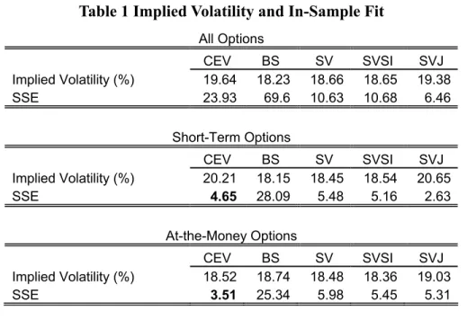
As shown in Table 1, we compare the testing results of the CEV model with those of

the BS, the SV, the SVSI, and the SVJ models obtained by Bakshi, Cao and Chen (1997).

In the all-option category, the SSE of the CEV model is lower than that of the BS model,

but higher than those of the SV, the SVSI, and the SVJ models. However, in short-term

options category, the CEV model has lower SSE than the those of SV and the SVSI models,

only higher than the SSE of the SVJ model. Furthermore, the CEV model performs best

even better than the SVJ model in at-the-money options category.

4.1.4 Assessment of the Relative Model Misspecification

As Rubinstein (1985) had done, the most popular diagnostic of relative model

misspecification is to compare the implied-volatility patterns of each model across both

moneyness and maturity

12

. The procedure is as follows: First, substitute the spot index and

interest rates of date t as well as the structural parameter values implied by all date (t-1)

option prices, into the option pricing formula, which leaves only the spot volatility

undetermined. Next, for each given call option of date t, find a spot volatility value that

equates the model-determined price with the observed price of the call. Then, after

repeating these steps for all options in the sample, obtain for each moneyness-maturity

category an average implied-volatility value.

Using the subsample data from July 1990 to December 1990 as Bakshi, Cao and

Chen (1997), the average implied volatilities of the CEV model are computed in Table 2.

In Figure 1, the implied volatility graph is presented. We then compare it with the results

by Bakshi, Cao and Chen (1997)

13

. For short-term calls, the CEV model still shows large

U-shaped moneyness-related biases. However, the magnitude of the biases, 6.5%, is only

slightly larger than that the SV model, around 6%. For medium-term and long-term calls,

the moneyness-related smiles of implied volatility are greatly reduced, and the

corresponding magnitudes are only 1.68% and 1.36%, respectively. We can also find that

the implied volatility of the CEV model in long-term options (maturity

≥ 180 days) is the

most stable case compared with other maturity-based options. For those options with

longer than 180 days to expiration, the implied volatility of the CEV model is more stable

than all of the other models including the SVJ model.

In sum, the CEV model is still subject to the model misspecification problems as all

of the option pricing models tested in Bakshi, Cao and Chen (1997). However, in terms of

the implied volatility, the extent of the moneyness-related biases is similar to the SV model,

and is much better that the BS model.

4.1.5 Out-of-Sample Pricing Performance

In out-of-sample option pricing, the presence of more parameters may actually cause

over-fitting and have the model penalized if the extra parameters do not improve its

structural fitting. For this purpose, Bakshi, Cao and Chen rely on the previous day’s option

prices to back out the required parameter/volatility values and then use them as inputs to

compute the current day’s model-based option prices. Next, they subtract the

model-determined price from its observed counterpart, to compute both the absolute and

the average percentage pricing errors and their associated standard errors. This prevents the

biases in the objective function (Eq 4.1.2) in favor of more expensive calls, such as

long-term and in-the-money calls. To make our results comparable with those of Bakshi,

Cao and Chen (1997), we also follow their approach by changing the objective function in

(Eq 4.1.2) to absolute pricing errors

(Eq 4.1.3)

∑

= Φ Φ ≡ N n n t V t V t APE 1 ), ( ] ), ( [ min ) (

ε

(Table 3)

and percentage pricing errors

(Eq 4.1.4)

∑

= Φ Φ ≡ N n n n n n t V C t K t V t PPE 1 ), ( ˆ ( , , ) ] ), ( [ min ) (

τ

ε

(Table 4) .

Pricing errors reported under the heading “All-Options-Based” are obtained using the

parameter/volatility values implied by all of the previous day’s call options; those under

“Maturity-Based” are obtained using the parameter/volatility values implied by those

previous-day calls whose maturities lie in the same category (short-term, medium-term, or

long-term) as the option being priced; those under “Moneyness-Based” are obtained using

the parameter/volatility values implied by those previous-day calls whose moneyness

levels lie in the same category (OTM, ATM, or ITM) as the option being priced.

In Table 3, we compare the out-of-sample pricing errors of the CEV model with those

of the BS, the SV, the SVSI, and the SVJ models from Bakshi, Cao and Chen (1997). We

mark those results of the CEV model which are better or equal to the results of the SV

model. In general, the out-of-sample pricing errors of the CEV model are in-between the

BS model and the SVJ model. In OTM and part of the ATM option cases (S/K <1.00), the

CEV model performs better than the SV model, while in the deep ATM and ATM options,

the CEV model has larger pricing errors than the SV model. In Table 4, percentage pricing

errors of the CEV model also show similar results as those of absolute pricing errors.

However, in Table 4, the CEV model performs slightly better in short-term (maturity<60)

and worse in long-term (maturity

≥ 180).

Finally, we should note that the CEV model only produces negative percentage

pricing errors for short-term OTM (

S/K ≤1.0

and days-to-expiration less than 60)

options. This is slightly different from the observation of Bakshi, Cao and Chen (1997) that

all models produce negative percentage pricing errors for options with

moneyness

S/K≤1.0

, and positive percentage pricing errors for options with

S/K ≥1.03

,

subject to time-to-expiration not exceeding 180 days.

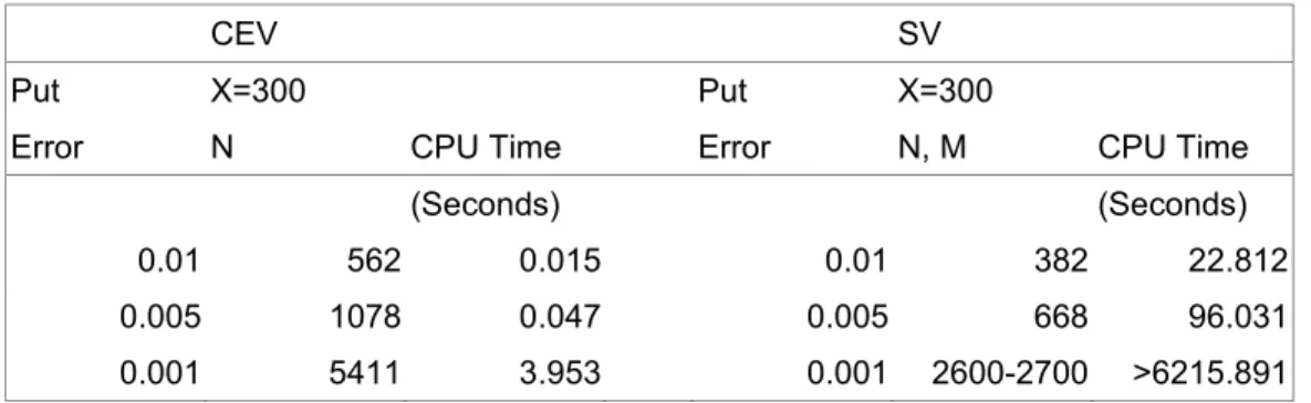
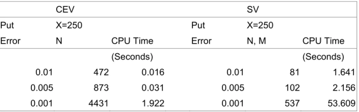
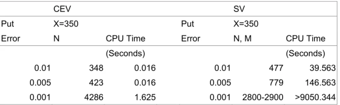
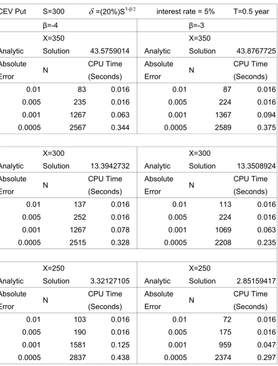
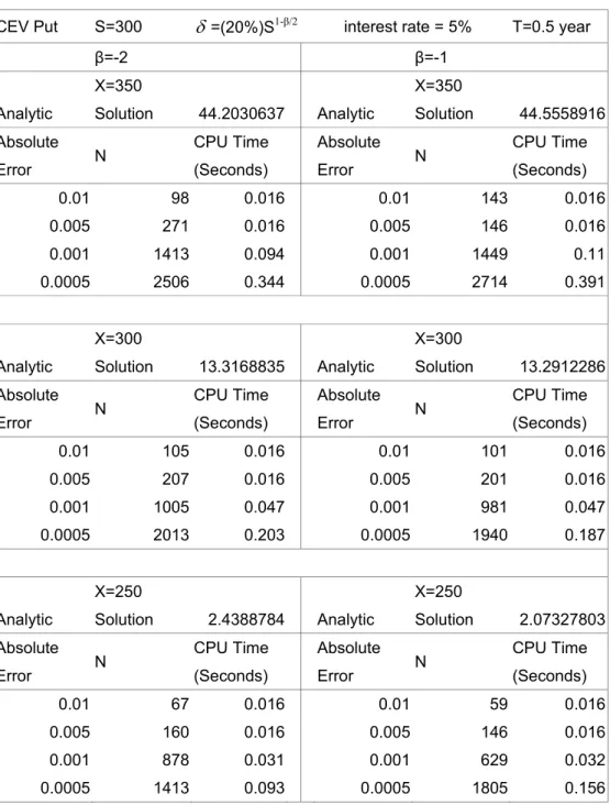
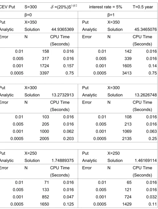
4.2 Pricing Performances of Numerical Procedures

In this section, we will compare the pricing performances of the CEV and the

stochastic volatility models in terms of cost-accuracy based analysis, namely, numerical

accuracy and computational efficiency. The numerical accuracy is measured by the

absolute pricing error between the option values generated by the numerical method and

the closed-form solution, given fixed CPU time. The computational efficiency is measured

by the required CPU time, given fixed pricing errors between the option values generated

by numerical method and the closed-form solution.

The numerical method of the CEV process we use is the trinomial model developed

by Boyle and Tian (1999). The numerical method of the stochastic volatility model we use

is the finite difference algorithm by Scott (1997).

14

4.2.1 The Trinomial Method Under the CEV Process

Boyle and Tian (1999) first transform the stochastic process under nature’s

probability measure into the Q-measure under which the deflated price processes of all

securities are martingales. The revised process is as follows:

(Eq 4.2.1)

dS

₌

rSdt

₊

_σ

S

β/2

dz

They first transform the variable

S

so that the transformed process has constant

volatility.

Let

y

=

y

( S

t

,

)

and apply Ito’s Lemma, the stochastic differential equation for y is

(Eq 4.2.2)

S dz S y dt S y S S y rS t y dy       ∂ ∂ +       ∂ ∂ + ∂ ∂ + ∂ ∂ = /2 2 2 2 2 1

_σ

β

_σ

β

To make the process (Eq 4.2.2) has constant volatility, they use the transformation

such that

v

S

S

y

₌

∂

∂

_σ

β/2

2 / β

σ

−

=

∂

∂

S

v

S

y

Therefore, this transformation is given by

(Eq 4.2.3)

₍

₎

1 /2

2

/

1

β

β

σ

−

−

=

v

S

y

for

β

≠

2

and the appropriate transformation

y

v

log(S

)

σ

=

for

β

=

2

.

For the case with

β

≠

2

, the transformed equation becomes

(Eq 4.2.4)

dy

rS

v

S

S

v

S

_

dt

+

vdz





















−

+

=

− /2 2 − /2−1

2

2

1

β β β

σ

β

σ

σ

(

)

y dt vdz v y r _ +      − −       − = 2 / 1 4 2 1 2

β

β

β

The transformed process above has constant volatility, which allows for a

straightforward construction of a two-dimensional grid for trinomial trees. However, this

transformed process has a complex drift term, which explodes when y approaches zero

(with the only exception when

β

=

0

). This makes the standard trinomial branching

process problematic for the region close to

y

=

0

, because the trinomial jumps and

probabilities must be chosen to match not only volatility but the drift.

They then modify the standard trinomial method as suggested by Tian (1994), in

which the trinomial branching process simultaneously utilizes both the transformed

process (Eq 4.2.4) and the original process (Eq 4.2.1). The detailed procedures can be

implemented in two steps as in the work by Boyle and Tian (1999).

4.2.2 The Finite Difference Method of the SV Model

The finite difference algorithm of Scott (1997) is briefly summarized as follows:

)

(t

S

,

t≥0

represents the price for a stock or a stock portfolio. Scott uses squared

Gaussian diffusions under actual measure:

(Eq 4.2.5)

dy(t)=[

κθ

−(

κ

+

λ

)y]dt+

γ

y(t)dZ(t)

,

15

where Z is Brownian motion and

λ

_j

=

0

for the risk-neutral process.

15 _{Note that there are slight differences by Scott’s notation in (Eq 4.2.5) and (Eq 4.2.6) compared with those} of Bakshi, Cao and Chen (1997) in (Eq A.2) and (Eq A.1).