1
行政院國家科學委員會專題研究計畫成果報告
※※※※※※※※※※※※※※※※※※※※※※※※※※※※※
匯率風險與跨時避險的研究(2/2)
※※※※※※※※※※※※※※※※※※※※※※※※※※※※※
計畫類別:個別型計畫
計畫編號:NSC 91-2416-H-002-001
執行期間:91年8月1日至92年7月31日
計畫主持人:洪茂蔚
處理方式:可立即對外提供參考
執行單位:國立台灣大學國際企業系
中華民國九十二年七月三十一日
2
In this project, we empirically investigate a simple version of international asset pricing model: ih m im m ii t f t i t V V V r r E ( 1) 2 1 , 1 ,+ − + =− +γ + γ − (1)
∑
∑
− + − + l l ih l m l l i l m V Vπ γ ω π ω γ ) (1 ) 1 ( where, =(∑
)/(∑
) l l l l l m W Wγ γ and∑
− − = l l l l l l W W ) 1 ( ) 1 ( γ γ ω .The following terms are used in the above and following discussion:
γ : Arrow-Pratt coefficient of relative risk aversion.
t
π : the price level at time t.
t i
R, : the real return for security i at time t.
N t i
R, : the nominal return for security i at time t.
t
C : the real consumption at time t.
N t
C : the nominal consumption at time t.
t m
R , : the real return for market portfolio at time t.
N t m
R , : the nominal return for market portfolio at time t.
t
W : investor’s nominal wealth at time t
Vcc : Vart(ct+1) jj V : Vart(rj,t+1)∀j =i,m Vcj :Covt(ct+1,rj,t+1)∀j=i,m Vim:Covt(ri,t+1,rm,t+1) π i V : Viπ =Covt(ri,t+1,rπ,t+1)
3 1 ,t+ rπ : 1 1 1 1 , ln( ) + + + + = = t t t t d d r ππ π π
∑
∞ = ++ + + − = 1 1 , 1 1 , ,( ) ) ( j j t m j t t t i t ih Cov r E E r V β∑
∞ = ++ + + − = 1 1 , 1 1 , ,( ) ) ( j j t j t t t i t ih Cov r E E r V π β πIn our model, inflation variable includes inflation risk and exchange rate risk. That is because inflation variable is priced under numeraire currency. Therefore, in addition to inflation risk that expresses inflation risk in domestic market, there exists exchange rate risk that indicates the risk of each currency relative to numeraire currency. If domestic inflation is a stable variable, the only random component in π is the relative change in the exchange rate between the numeraire currency and the investor’s home currency. Then, Vilπ is a pure measure of the exposure
of asset i to the exchange risk and l ih
V π is a measure of the exposure of asset i to hedge against the
exchange risk of the country in which investor l resides.
We adopt the Vector Auto-Regressive (VAR) approach of Campbell (1991) and construct a state variable system to estimate the market hedging portfolio and the currency hedging portfolio. We assume that the world market index return, r , is the first element of a K -element state m
variable vector z and the currency deposit return, t l e
r , is the l+1st element, l =1,2,...,L. The other elements of z are known to the market at the end of period t and are related to the t
forecasting of future world market returns and currency deposit returns. In addition, we assume that all the variables zt are demeaned and that the vector z follows a first order VAR. t
zt+1=Ψzt +ut+1, (2)
4
first-order is not restrictive because a higher-order VAR can always be stacked into first-order companion form as discussed by Schwarz (1978). Then we can use the first order VAR to generate simple multi-period forecasts of future returns as,
t i i t t z z E 1 1 + + + =Ψ . (3)
Define a K -element constant vector 1e whose first element is one and the other elements are all
zero. Then, rm,t =e1′zt and ,+1− m,t+1 = 1′ t+1
t t
m Er e u
r . Define another K -element constant vector
el whose l+1st element is one and other elements are all zero. Then, t l t e elz r, = ′ and 1 1 , 1 ,+ − + = ′ t+ l t e t l t e Er elu r .
It follows that the discounted sum of forecast revisions in world market returns is,
∑
∑
∞ = ∞ = + + + +− = ′ Ψ 1 1 1 1 , 1 ) 1 ( j j t j i j t m j t tE E β r e β u (4) =e1′βΨ(I−βΨ)−1ut+1 = ′θh tu+1 , where, θh′ is defined as 1 ) ( 1′βΨ I−βΨ −e which measures the importance of each state variable in
forecasting future returns on the world market.
Similarly, the discounted sum of forecast revisions in currency deposit returns is,
∑
∑
∞ = ∞ = + + + +1− ) 1 , 1 = ′ 1 Ψ 1 ( j j t j i l j t e j t tE E β r el β u (5) 1 1 ) ( − Ψ − + Ψ ′ =elβ I β ut5 =θe′l′ut+1 , where, θe′l′ is defined as 1 ) ( − Ψ − Ψ ′β I β l
e which measures the importance of each state variable
in forecasting future returns on the currency deposit.
Equation (1) appears to be the natural relation to use in an empirical investigation of an international asset pricing model because it takes into account the investor’s use of newly acquired information in creating a portfolio, thus taking into account his hedging strategy. The model requires equation (1) to hold for every asset including the market portfolio, market hedging portfolio, currency portfolio and currency hedging portfolio. Therefore, we assume that each asset return satisfies the following system of pricing restrictions :
+ +
∑
=∑
= − + − + − + + − = − L l l eh l L l l e l h m t f t t V V V V V r r E 1 1 1 1 1 1 11 1 , 1 , 1 ( 1) (1 ) (1 ) 2 γ γ γ ω γ ω (6) M + +∑
=∑
= − + − + − + + − = − L l l Neh l L l l Ne l Nh Nm NN t f t N t V V V V V r r E 1 1 1 , 1 , ( 1) (1 ) (1 ) 2 γ γ γ ω γ ωwhere, we replace V and iπ Viπh in equation (1) with V and ie V because the empirical evidence ieh
shows that fluctuations in domestic inflation are almost negligible relative to exchange rate changes.
Let rt denote the N ×1 time series vector which includes N risky assets, ri∀i=1,...,N. In matrix notation, equation (6) and equation (2) can be re-expressed in terms of random log excess return as,
6 + − + − + − + + − Φ = ⋅ − − t t t eh t e t h t m t d t t f t t u h h h h h z i r r z ξ γ γ γ γ , , , , , 1 , ( 1) (1 ) (1 ) 2 1 (7) ) , 0 ( ~ | t 1 t t t t I N H u − = ξ ε , = + × + × × × × 22 21 12 11 ) ( ) ( : N N K N N K K K t H H H H N K N K H
where, i is an N ×1 vector of one, Ht is the conditional covariance matrix of asset returns, hd t, is the diagonal element of 22
N N
H × which denotes the conditional variance of each risk asset, hm t, is
the 1st column of HN21×K which denotes the conditional covariance of each asset with the market
portfolio,
∑
= = K k t k k h t h h h 1 , ,, θ denotes the conditional covariance of each asset with the market hedging portfolio,
∑
= + = L l t l l t e h h 1 , 1, ω denotes the conditional covariance of each asset with the currency portfolio,
∑
∑
= = = K k t k l k e L l l t eh h h 1 , , 1, ω θ denotes the conditional covariance of each asset with the currency hedging portfolio, hk,t is the k th column of HN21×K and hl+1,tis the l+1st column of
21
K N
H × .
Three tests of asset pricing restrictions as special cases of equation (7) are implemented. First, we test the validity of the conditional CAPM that implies that γ must be significantly different from zero. The null hypothesis of γ =0 is tested against the alternative hypothesis γ ≠0. Second, the test of market hedging risk, exchange risk and exchange hedging risk as an important factor in the asset pricing model is implemented. This test implies that γ is not equal to one in equation (7). Otherwise, risk premia of assets are determined only by the covariance with the market portfolio. As discussed in the theoretical model, if we only test the price of market hedging risk, V , and ih
7
currency risk, V , we can find that the two risk values will be significant or insignificant ie
simultaneously because they all depend on whether or not relative risk aversion, γ, is different from one. Hence, we ultimately want to know which risk is most important in terms of scale.
Equation (7) follows directly from the system of the international asset pricing model. To implement the tests of the above hypotheses, the dynamics of the variance-covariance structure in equation (7) must be specified. A multivariate GARCH process based on the work of Ding and Engle (1994) is used to obtain a testable version of the model.
For simplicity, we assume that the innovation vector εt follows a popular GARCH(1,1) process. The time-varying conditional covariance matrix therefore can be parameterized as,
Ht = +Γ aε εt−1 t′ ′ +−1a bHt−1b′, (8)
where, Γ, a ,and b denote (N+K)×(N+K) matrices of parameters. It is difficult to estimate the model due to the large number of unknown parameters. In practice, it is necessary to further restrict the specification for Ht to obtain a numerically tractable formulation. One useful special
case is to assume that both a and b are restricted to be diagonal matrices. In such a parameterization, the conditional covariance between εi t, and εj t, depends only on past values of
εi t, −1⋅εj t, −1, and not on the products or squares of other residuals. Therefore, equation (8) can be written in a simple form:
Ht = +Γ αα ε ε′∗ t−1 t′ +−1 ββ′∗Ht−1, (9)
8
the symbol ∗ denotes the Hadamard (element by element) matrix product. However, the diagonal assumption is still too difficult to estimate, unless we can again reduce the number of unknown parameters. To this end, we assume that the εt process is covariance stationary following Ding
and Engle (1994). Consider the following system of equations,
1 t t | t 1 ~ (0, t) t t t t t H N I r z E r z − − + = ε ε (10)
If the εt process is covariance stationary, its unconditional variance-covariance
matrix is equal to,
H0 =Γ∗(ii′−αα′−ββ′)−1. (11)
Then, equation (9) is replaced by,
Ht = H0∗ ′ −(ii αα ββ′ − ′ +) αα ε ε′∗ t−1 t′ +−1 ββ′∗Ht−1. (12)
In a covariance stationary and diagonal construction with (N+K) assets, the number of unknown parameters in the conditional variance equation is reduced to 2(N+K) . The unconditional variance-covariance matrix, H , is not directly observable. Here we set it equal to 0
the sample covariance matrix of the return.
We use monthly dollar denominated index returns for U.S., U.K., Germany, Japan, and the world portfolio as reported by Morgan Stanley Capital International (MSCI) to investigate the proposed international asset pricing model. The sample period is from January 1980 through December 1997. We also use Eurocurrency rates offered in the interbank market in London for
9
one-month deposits in U.S. dollars, U.K. pounds, German DM and Japanese yen.
Table I reports the summary statistics for log index returns on both equity and Eurocurrency rates computed in U.S. dollars in excess of returns on the Eurodollar rate. The summary statistics include means, standard deviations, skewness, kurtosis, Bera-Jarque(1982) statistics, and the sample correlation. The magnitudes of the means, volatilities and correlations are very similar to those previously documented in other studies. The kurtosis values indicate that the unconditional distribution of excess log returns has heavier tails than the normal distribution for all countries. Furthermore, the Bera-Jarque statistics also show that the hypothesis of normality is rejected in our sample. Hence, we incorporate the heteroskedastic property when we estimate the asset pricing model.
Descriptive statistics for the state variables are reported in the second panel of Table I. We select a set of state variables that have been widely used in the literature. These instruments include the logarithm of the monthly MSCI world dividend yield (DIV) and the one-month U.S. T-bill rate (TB) both in excess of the monthly Eurodollar rate. These variables have been found to measure the information that investors use to set prices in the market. For example, Campbell (1996) finds that the dividend yield has some predictive power for future stock returns. Similarly, Fama and Schwert (1977), Ferson (1989), and Ferson and Harvey (1991) find that the short-term T-bill rate (TB) is capable of predicting monthly returns of stocks and bonds.
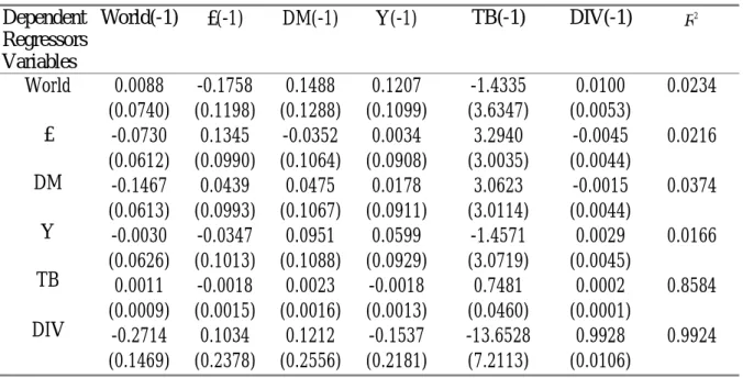
We first construct the dynamic behavior of state variables. Table II reports the estimates of the coefficients in the one-lag VAR. The first row of Table II reports the monthly forecasting equation for the excess log return of the world market portfolio (World). Since there is little serial correlation in the monthly world market log return, the coefficient for the World (-1) is small and insignificant. However, the coefficient for world dividend yield (DIV) is significantly positive and
10
the short-term T-bill rate (TB) is negative. The second row of Table II gives the monthly forecasting equation for the return on the currency deposit, £. The coefficient of lagged currency deposit returns is also small and insignificant. The remaining rows of Table II report the dynamics of the state variables. It can be seen that DIV behaves like a persistent AR(1) process with a coefficient of 0.9928.
The intertemporal model applied to international financial markets implies that the conditional expected log return on any asset is linearly related to the covariance of asset return with world market return, the covariance with news about the discounted value of all future market returns i.e. the hedging portfolio return, the covariance with the currency deposit return, and the covariance with news about the discounted value of all future currency deposit returns i.e. the currency hedging portfolio return. If the world market risk, news about the discounted value of all future market risk, exchange risk, and news about the discounted value of all future exchange risk are the only four relevant factors, the price of covariance risk γ should be significantly positive and significantly greater or less than one. It should also be noted that the value of γ should not be equal to zero or one.
In order to avoid the measurement error, the econometric system employed simultaneously estimates the parameters of VAR and the asset pricing model. The results are reported in Table III. Consider the estimates of parameters in the VAR. All the elements in the parameter matrix are similar to the unconstrained estimates that are reported in Table II. The estimate of γ is 3.0884 which is significantly different from zero. This implies that the conditional expected international asset return varies with world market volatility. This evidence supports the conditional version of the international CAPM. Next, consider the estimates of parameters in the multivariate GARCH process. All elements of vectors α and β are statistically significant at any conventional level. Moreover, the estimates satisfy the stationary conditions, α αi j+β βi j <1 ∀i j, , for all the
11 variance and covariance processes.
If the estimate of γ is equal to one, the model collapses to the conditional CAPM. Since we have the unrestricted estimates, a Wald test would be a convenient way to proceed. The value of the criterion function is χ2( )1 =21.935, which corresponds to a p-value of 0.000. This implies that we can reject the hypothesis that market hedging demand, exchange risk, and currency hedging demand are not important factors in pricing international stock returns. In other words, the conditional expected international asset return varies with market volatility, market hedging volatility, currency volatility and currency hedging volatility simultaneously. This evidence supports the international version of the intertemporal asset pricing model.
The price of risk that arises from the traditional covariance of an asset’s return with world
market return is
∑
= − + − + L l l e h 1 1 1 (1 ) ) 1 (γ θ γ θγ , where θh1 is the first element of θh and l e1
θ is the first element of θe. Therefore, this model provides a distinct link between the coefficient of relative risk aversion, γ , and the various prices of risks.
We use an econometric method to examine whether or not relative risk aversion, γ , is different from one. The result shows that three risk components, which depend on whether or not the value for relative risk aversion, γ , is different from one, all significantly explain the cross-section of equity returns in the U.S., U.K., Germany and Japan. However, we would like to know their relative importance. Table IV reports the mean of the risk variables for the U.S., U.K., Germany, and Japan equity markets. The traditional international CAPM uses only the market risk and exchange risk to price assets, whereas the intertemporal model also compensates for market hedging risk and exchange hedging risk. Table IV shows some striking results about the risk characteristics of international equity returns. First, we compare the market risk premium and the
12
exchange risk premium for our equity markets. For the U.S. equity market, the market risk is very important for explaining return whereas the exchange risk is small and not significant. In the other three equity markets, we find that although exchange risk is less important than market risk, it is still an important factor to explain equity market return. These findings are consistent with Dumas and Solnik (1995) and De Santis and Gerard (1998) who also find that exchange risk is important for pricing international equity returns.
Second, Dumas and Solnik (1995) claim that exchange risk might be proxying for market hedging risk. Table IV also allows a comparison of the magnitudes between market hedging risk premium and exchange risk premium. Except for the U.S. equity market, the exchange risk premia are highly significant relative to market hedging risk premia. This might be because we use the U.S. dollar as a currency measure, so exchange risk become less important for the U.S. equity market. Hence, we can conclude that if PPP is violated, exchange risk is a more important factor than hedging risk in the international asset pricing model. This implies that the conclusion of Chang and Hung (1999) and Hodrick, Ng, and Sengmueller (1999) which states that hedging risk is important in the international asset pricing model should be reassessed in the presence of exchange risk.
Third, DeSantis and Gerard (1998) explain the negative exchange risk since one would be willing to give up larger expected returns for smaller expected returns because currency can provide a hedge to PPP deviation. However, this is a relationship of contemporary hedge. Table IV shows that market risk premium is positive, market hedging risk premium is negative, exchange risk premium is negative except for U.S. , and exchange hedging risk is positive. In addition to contemporary hedge between exchange risk premium and market risk premium, market hedging risk premium and exchange hedging risk premium are two intertemporary hedges to market risk premium and exchange risk premium. That is because future market return and future currency can provide a hedge to currency market return and currency return.
13
Table I
Weightsa Mean(*100) S.D.(*100) Skewness Kurtosis B-J U. S. U.K. Germany Japan World 0.35 0.11 0.04 0.31 1 0.3283 0.2540 0.1934 0.1374 0.2255 4.3762 5.8702 6.1322 7.0080 4.2165 -1.0290** -0.4888* -0.4682* 0.0385 -0.7831* 5.0485** 1.9517** 1.3120* 0.3476* 2.4313** 266.2657** 42.6871** 23.2785** 1.1354* 74.9264** * and ** denote statistical significant at the 5 % and 1 % level, respectively.
a as of December 31,1990.
Instrumental Variables
Mean(*100) S. D.(*100) Maximum Minimum World(-1) £(-1) DM(-1) Y(-1) TB DIV 0.2173 0.0518 -0.1401 0.0462 -0.1078 -90.0291 4.2076 3.4764 3.5097 3.5450 0.0901 31.0668 10.5096 14.2591 7.8664 10.9511 0.0441 -4.2420 -20.1767 -12.6903 -10.8948 -11.0821 -0.3916 -146.9676
14
Table II
Dependent Regressors Variables
World(-1) £(-1) DM(-1) Y(-1) TB(-1) DIV(-1) R2
World £ DM Y TB DIV 0.0088 (0.0740) -0.0730 (0.0612) -0.1467 (0.0613) -0.0030 (0.0626) 0.0011 (0.0009) -0.2714 (0.1469) -0.1758 (0.1198) 0.1345 (0.0990) 0.0439 (0.0993) -0.0347 (0.1013) -0.0018 (0.0015) 0.1034 (0.2378) 0.1488 (0.1288) -0.0352 (0.1064) 0.0475 (0.1067) 0.0951 (0.1088) 0.0023 (0.0016) 0.1212 (0.2556) 0.1207 (0.1099) 0.0034 (0.0908) 0.0178 (0.0911) 0.0599 (0.0929) -0.0018 (0.0013) -0.1537 (0.2181) -1.4335 (3.6347) 3.2940 (3.0035) 3.0623 (3.0114) -1.4571 (3.0719) 0.7481 (0.0460) -13.6528 (7.2113) 0.0100 (0.0053) -0.0045 (0.0044) -0.0015 (0.0044) 0.0029 (0.0045) 0.0002 (0.0001) 0.9928 (0.0106) 0.0234 0.0216 0.0374 0.0166 0.8584 0.9924 Standard errors are in parentheses.
15
Table III
γ 3.0884 (0.4459) α β rm t, −rf t, £ DM Y TB DIV 0.2102 (0.0233) 0.1674 (0.0307) 0.1936 (0.0432) 0.1902 (0.0233) 0.2100 (0.0200) 0.1753 (0.0410) 0.9602 (0.0085) 0.9755 (0.0147) 0.9507 (0.0208) 0.9677 (0.0083) 0.9605 (0.0076) 0.9512 (0.0267) U.S. U.K. Germany Japan 0.2138 (0.0475) 0.1561 (0.0197) 0.3063 (0.0270) 0.3054 (0.0286) 0.9250 (0.0331) 0.9805 (0.0093) 0.9484 (0.0098) 0.9506 (0.0096)16
Table IV
Summary of Risk Premiums
TP MP MHP CP CHP U.S. Mean Std. Dev. U.K. Mean Std. Dev. German Mean Std. Dev. Japan Mean Std. Dev. 4.3681 1.0023 5.1384 1.1164 4.3776 1.3628 6.7094 1.7167 5.4035 1.7551 6.9687 1.7529 5.6133 1.7056 8.0265 2.2407 -1.3546 1.3885 -1.2515 1.3188 -0.2906 1.4192 -0.7827 1.5124 0.0579 0.2067 -0.7548 0.2218 -0.9761 0.2919 -0.9013 0.2163 0.2610 0.2118 0.1760 0.2401 0.0316 0.2468 0.3688 0.2773
17
REFERENCES
Adler, M. and B. Dumas. (1983), "International portfolio selection and corporation finance: a synthesis." Journal of Finance , 38, 925-984.
Bansal, R. D. A. Hsieh, and S. Viswanathan. (1993), "A new approach to international arbitrage pricing." Journal of Finance , 48, 1719-1747.
Bera, Anil K. and C. M. Jarque (1982), "Model specification tests : a simultaneous approach." Journal of Econometrics, 20, 59-82.
Campbell, John Y. (1991), "A variance decomposition for stock returns." Economic Journal, 101, 157-179.
Campbell, John Y. (1993), "Intertemporal asset pricing without consumption data." American Economic Review, 83, 487-512.
Campbell, John Y. (1996), "Understanding risk and return." Journal of Political Economy, 104, 298-345.
Carrieri, F. (2001), "The Effects of Liberalization on Market and Currency Risk in the European Union." Forthcoming, European Financial Management.
Chang J. R. and Hung M. W. (1999), "An International asset pricing model with time-varying hedging risk." Working paper.
Cumby, R.E. (1990), "Consumption risk and international equity returns: Some empirical evidence." Journal of international Money and Finance, 9, 182-192.
De Santis G. and Gerard B. (1997), "International asset pricing and portfolio diversification with time-varying risk." Journal of Finance , 52, 1881-1912.
De Santis G. and Gerard B. (1998), "How big is the premium for currency risk?" Journal of Financial Economics , 49, 375-412.
Dumas, B. and B. Solnik (1995), "The world price of foreign exchange risk." Journal of Finance , 50, 445-479.
18
consumption and asset returns: a theoretical framework." Econometrica, 57, 937-969.
Epstein, Larry G., and S. E. Zin (1991), "Substitution, risk aversion, and the temporal behavior of consumption and asset returns: an empirical analysis." Journal of Political Economy, 99, 263-286.
Fama, E.F., and G.W. Schwert, (1977), "Asset returns and inflation." Journal of Financial Economic, 5, 115-1461.
Ferson, W. (1989), "Changes in expected security returns, risk, and the level of interest rates." Journal of Finance , 44, 1191-1217.
Ferson, W. and C. R. Harvey. (1991), "Variation of economic risk premiums." Journal of Political Economy , 99, 385-415.
Ferson, W. and C. R. Harvey. (1993), "The risk and predictability of international equity returns." Review of Financial Studies, 6, 527-567.
Giovannini, Alberto, and P. Weil (1989), "Risk aversion and intertemporal substitution in the capital asset pricing model." NBER, 2824.
Harvey, C. R. (1991), "The world price of covariance risk." Journal of Finance , 46, 111-157. Hodrick, R. J., D. Ng and P. Sengmueller, “An International Dynamic Asset Pricing Model,” Working paper, Columbia University.
Kreps, D. and E. Porteus (1978), "Temporal resolution of uncertainty and dynamic choice theory." Econometrica, 46, 185-200.
Korajczyk, R. and C. Viallet. (1989), "An empirical investigation of international asset pricing." Review of Financial Studies, 2, 553-585.
Merton, Robert C. (1973), "An intertemporal capital asset pricing model." Econometrica, 41, 867-887.
Narayana, K. (1990), "Disentangling the coefficient of relative risk aversion from the elasticity of intertemporal substitution: an irrelevance result." Journal of Finance , 45, 175-190.
Ross, S. A. (1976), "The arbitrage theory of capital asset pricing." Journal of Economic Theory, 13, 341-360.
19
Solnik, Richard E. (1974), "An equilibrium model of the international capital market." Journal of Economic Theory, 8, 500-524.
Stulz, R.M., (1981), "A model of international asset pricing." Journal of Financial Economics, 9, 383-406.
Stulz, R.M., (1984), "Pricing capital assets in an international setting: an introduction" Journal of International Business Studies, winter, 55-73.
Svensson Lars E. O. (1989), "Portfolio choice with non-expected utility in continuous time." Economics Letters, 30, 313-317.
Weil, Phillippe (1989), "The equity premium puzzle and the risk free rate puzzle." Journal of Monetary Economic, 24, 401-421.