Hepatitis B virus mutants associated with hepatitis b surface antigen loss: Chicken or egg?

(1)

An Efficient Method of Solving Problems of Classification and

Selection Using Minimum Spanning Tree in

a

Flexible Manufacturing System

Pei-Sen

Liu

and

Li-Chen

Fu

Department of Computer Science & Information Engineering

National Taiwan University, Taipei, Taiwan, R.O.C.

Abstract

Flexible manufacturing systems (FMS’s) become more and more popular nowadays in the field of manufacturing since they can perform different workpieces automatically in more than one sequence and, hence, possess considerable flexibility. Design of an FMS will involve several levels of consideration and each level will endeavor to solve various problems. One of those levels is planning and scheduling where problems regarding how to perform ckzssifrcotzon and selection are intrinsic ones. In this paper, an efficient heuristic method by building some minimum spanning tree(s) (MST) to solve these problems is proposed and, then, it is applied to three different types of environment for illustration. Computer simulation results show that our approach can obtain a satisfactory solution in moderate computational time.

I. Introduction

Flexible manufacturing systems (FMS’s) become more and more popular nowadays in the field of manufacturing since they can perform different workpieces automatically in more than one sequence and, hence, possess considerable flexibility. In other words, no human intervention will be needed in determining system operations and in handling con- tingent incidents in such an automatic manufacturing environment. Design of an FMS will involve several levels of consideration and each level will endeavor to solve various problems. One of those levels is planning and scheduling where problems regarding how to perform clussifrcution and selection are intrinsic ones. In this paper, a efficient approach for solving these problems is proposed and is, later, applied to three different types of environment for illustration.

The first environment contains problems of so called group technology (GT) (see in [1]-[3]. Its philosophy is to perform necessary operations of processing a part by a group (cell) of machines which are physi- cally close-by as much as possible in o d e r to minimize the total handling time. Before such a technology can be applied, all the parts to be pro- duced in a machine shop with lots of machines have to be sorted out into several families. Each family of parts is formed by judging the degree of similarity in size, geometry, method of manufacture, etc. Above all, all the operations involved in each family should be related to only a particular group of machines. Obviously, these are also known as classification problems.

The second one is tied with problems of the so called process plan selection [5][6]. Due to the very flexibility of an FMS, for each part there exists a number of different process plans and each plan specifies different requirements for tools, auxiliary devices, as well as operations (for example, machining operations) to be performed altogether at a

given cost. Moreover, since there usually will be several parts to be manufactured at the same time, there may exist a contlict in using a single machine for manufacturing more than one part due to the choice of some possible combination of so many relevant process plans. Therefore, a mission for the production planner is to select one out of all possible combinations of all process plans so that the minimum number of fixtures, grippers, fedders, and tools will be required. In another words, the corresponding total cost will be the minimum over all possible choices.

Very often in a realistic situation, not only a subset of a set of process plans has to be chosen but also the sequence among process plans in that chosen subset has to be determined as well. This constitutes the third

environment to be considered here where the class of problem, originated from that mentioned above, is terms as process plan sequencing problems. Of c w m , the sequence to be selected here w i l l correspond to the minimum total cost as has been requested previously.

All these problems mentioned so far are NP-complete and, hence, the complexity of solving these problems is considerably high if its so

called “optimal” solution is attempted. Thus, introduction of some good heuristics which can reduce complexity will be preferable in solving these problems in real practice. The efficient approach proposed here is based on the concept of minimum spanning tree [4] mixed with some relevant heuristics. For illustration of the performance, some computer simulation examples are provided with satisfactory results.

II. Problem Formulations

A. Group Technology Problem

Group technology is an approach that seeks to identify those attributes of a population that permit its members to be collected into groups, sometimes called families, so as to take advantages of their similarities in manufacturing and design. In a manufacturing system part similarities are

of two types: design attributes (such as geometric shape and size) and manufacturing attributes (the sequence of processing steps required to make the part). Suppose there rue k parts, p,

.

. . h, which need to be manufactured and each part has m attributes. Then a kxm matrix PI can be built to indicate the parts’ information. Every entry PI,, is a number or a character, which represents the value of ith attribute of part p.. For illustration, table 1 shows the information about ten parts each of which has twelves attributes.

Since each attribute has different effect to identifymg a part, the Hamming distance has been modified by introducing the weight coeficient w; for each attribute i. Recall that the weighted Hamming distance between any two parts, say, p, and pb is defined as:

(2)

arm1 sur2 all13 alu4 aim5 anr6 I 9 0 1

,

4.0 3 4 B A 1 1 59 R G 1 8 8 Y Y 2.9 B C I aIu7 10 2.7 62 -1 2.7 am8 1 2 3 4 ~ u ' H = 5 6 7 8 9 IO am9

-

0 13.5 14.7 7.3 11.6 12.5 7.8 6.2 10.5 13.5 0 4.8 9.4 9.9 6.5 12.3 7.3 7.4 14.7 4.8 0 ' 6.4 7.1 6.8 12.5 10.5 7.8 7.3 9.4 8.4 0 7.3 11.2 12.1 6.9 11.6 11.6 9.9 7.1 7.3 0 8.7 14.4 8.6 9.7 12.5 6.5 6.8 11.2 8.7 0 12.3 S.5 9.4 7.8 12.3 12.5 12.1 14.4 12.3 0 10.0 6.9 6.2 7.3 10.5 6.9 8.6 8.5 10.0 0 7.1 10.5 7.4 7.8 11.6 9.7 9.4 6.9 7.1 0 9.2 7.5 7.7 5.9 10.8 13.3 10.0 9.6 11.5

-

amlo attrl 1 awl 2

Table1 Example]: Tuelre Allribules for Tcn Parts.

where di is the difference of the ith attribute between the two parts. Based on the part information matrix PI, we can first calculate the Ham- ming distance between every pair of parts, then a weighted Hamming distance matrix WH which indicates the degree of difference among every parts can be created accordingly. Thus, based on the part information matrix, we define the weighted Hamming distance matrix WH of which each entry, say, (ab) denotes the weighted Hamming distance between part pa and pb. Accordingly, the matrix WH registers the degree of dis-

similarity among all parts. For example, table 2 is the weighted Ham- ming distance mahix associated with the part information matrix shown in table 1. In this special case, if the ith attribute is a numerical value, then

4

= I Pki-PIb, I , else 4=0 when PI,=PI, and di=l otherwise.

By these definitions, a group technology problem can be stated as:

Given a kxk weighted Hamming distance matrix

WH,

group those k parts

into f families where f is a given number.

B.

Process Plan selectioa Problem

Most of the planning methods for automated manufacturing systems are based on the assumption that for each part there is only one process plan (defined as a sequence of operations) available. But in practical situation (e.g., in an FMS) one can generate a set of different process plans, whose attributes as well as costs may vary from one to the others. The former are defined as the auxiliary devices (such

as

fixtures, grippers, feeders. and tools) that each plan specifies whereas the latter is the manufacturing cost induced by that particular plan. By this observation, every process plan can be identified with its attributes (i.e., required auxiliary devices) and the associated cost. Suppose there are n auxiliary devices in a manufacturing system and at certain time there are p process plans to manufacture k parts, then the following incidence row vector is defined for each process plan Pi,

la9

:

x, = [X,i.X2,.

.

' ' J " i ]

Where

1 if the auxiliary device t is used in Pi 0 otherwises

and a row vector C is used to denote costs of all the process plans, i.e.,

c

= [Cl,C,, . ' ' .C,I

where Ci is the cost for process plan Pi. An example for demonstration is shown in figure. 1.

Like the first class of problems, after figuring out the incidence vector for each process plan, we can then construct a pxp weighted Ham- ming distance matrix D measuring dissimilarity among the plans. Each entry

4,

denotes the weighted Hamming distance between process plan Pi

and Pj. Now the process plan selection problem can be defined as follows: Choose from the set U={l,

...,

p ) a subset S=(j,,

,...,

j,) which contains one representative process plan j, for each part i, lSjiSp, i=l,

...,

k,

such that the following is minimized:

C

4,,.je+

CCi, (1)

CJil.j,)€As JiES

where As={(jl,j2), (j,,j3),

..., (jk-l,jk)).

In words, to manufa- k parts we choose from the set of p process plans a subset of k process p l w (counting the multiplicity) such that the total costs of these chosen p l w plus a measure dissimilarity over those plans is minimized.

c.

p r e s s plan sequencing h o b l e m

The class of problems considered here is originated from that given in subsection B but also takes into account the importance of the process- ing order of the manufacturing plam selected. This additional considera- tion will become imperative when the setup efforts caused by switching from one process plan to another are comparable to the total costs of the relevant process plans.

By

use of the previous notation, we now formulate the problems as follows: Corresponding to the subset S=(jl,

...,

jk), we define the set of

all possible permutations of the ordered kth tuple

GI,

...,

jk) as

n(S)

of which each element is denoted as n=(il,

...,

ik)En(S). Then, the objective is to minimize

C

dj,,d,, + CCji (2)

( i , & ) ~ W ) j,ES

where B(n)={(il,i2), h i 3 ) ,

...,

(ik-l,ik)) over

all

possible S c

U

and all possible n(S).

m.

Solving Problems of Classification and Selection Using Modified MST In section 2, we have formulated the three classes of problems to be studied here. Later in this section we will show that by simply introducing some suitable m&cations to the MST according to the problem nature, all these problems can be solved efficiently. It is noteworthy, however, that certain heuristics will have to be introduced when Concepts

10 9.2 7.5 7.7 5.9 10.8 13.3 10.0 9.6 11.5 0

2149

(3)

‘1 ‘2 ‘3 ‘4 ‘ 5 ‘6 ‘7 ‘8 ‘9 ‘IO

~ - [ ~ . 8 . 9 . 4 . 1 1 . 6 . 5 . 7 . 3 . 4 . 4 . 3 , 5 . 1 . 6 . 4 . 5 . 2 . ~ . ~ 1 ~i~~~~ 1. ~ ~ ~Ten Process Plans associaled nilh Four Parts. ~ ~ 1 ~ 2 :

of MST are to be used to solve these NP-complete problems in general. Hence, the optimalily of solutions will be traded with the efficiency of reaching good solutions.

A. Group Technology F’roblem

Recall that this class of problems are characterized mainly by the

weight Hamming distance matrix WH. The objective is to group k parts in total into f families. Then, it is quite straightforward to build a graph G=(V,E) according to the mauix WH. Specifically, V corresponds to the set of parts and each element of E, say, (v,w) denotes the weighted edge between the part py and pw Now we are ready to propose an approach of solving the problems in the following:

Algorithm A

Stepl: According to the weighted Hamming distance matrix WH, build a corresponding undirected complete graph G=(V,E). Create a minimum spanning tree S=(V,T) of G. For index = I to f-1 do Step3.1 and Step3.2: Step3.1:

Step3.2:

Now the graph S=(V,T) is an unconnected graph with f com- ponents.

Step2: Step3:

Choose an edge (v ,w) in T of the largest weight; Delete (v ,w ) from T.

Step4:

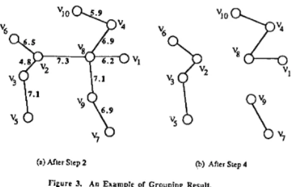
After a minimum spanning tree is constructed in Step2, (f-I) edges of the tree with the larger weights are deleted so that S becomes an unconnected graph with f components. Each component thus corresponds to a family of parts. For example, there are totally ten parts which are shown in table 1 and table 2, and they are to be grouped into three families. Figure 3 shows the partial and the final result of our approach where

three families are found as:

Remark: To balance the load of these families the above algorithm should be modiIied to meet this constraint. At first an integer number lp indicating the lowest number of parts in every family must be given (or be calculated by some rule), then Step3 can be modified as follows (the

lpz,ps.ps.p61. and {pr,psl.

(a) Gragh G=(V,E) @) A M i n i ” Spanning Trce Of G

Figure 2. A n Elample or Minimum Spanning Tree.

(a) After Step 2 @) Ahcr Step 4

Figure 3. An Example of Grouping Resuit.

other steps remain unchanged): When the next largest edge is chosen, we must check after deleting this edge whether there exists a subtree whose number of node is less than lp, If it is, then this edge must be kept, and

is deleted it otherwise. As before, after deleting f- 1 edges Step3 is then terminated.

B. Process Plan Selection Problem

The problems to be considered here are not only characterized by a weighted Hamming distance matrix D (as before) but also a cost vector C of all relevant process plans and a variable k which indicates the number of total parts. Likewise, an undirected graph G=(V,E) is constructed according to the matrix D and the vector C as well, where V now denotes the set of process plans whereas the weight of each edge in E, say, (v.w) is defined as

C k

I (v.w) I = C , + C , + ~ d , , = C,+C,+k&w 2

(k-1) (3)

where C; denotes the number of 2-combinations of a k-set. The choice of the weight function is due to the fact that the total weight of any solution tree (with (k-I) tree branches) out of the graph G will generally be more close to the value given hy the objective function in (1) than when d,, instead of -d,w is used in the calculation (3). Based on the graph, a modified MST is constructed and gives a desired result. The detailed algorithm is shown below:

c2“

k- I

Algorithm B-1:

Stepl: According to the pxp weighted Hamming distance matrix D, the number of parts to be processed k. and the cost vector C, do Stepl.1 and Stepl.2 to build an undirected complete graph G=(V,E).

Stepl.1: For each process plan Pi builds a vertex Vi in V so that the number of vertices in V is p.

Stepl.2: The weight of the edge (v.w) is given by (3). Let F be a set called forest, which is a set of trees. Initially, F

is set to be empty.

Do Step3.1 through Step3.3 repeatedly until F becomes a tree with k vertices.

Step3.1:

Step3.2: Delete (v,w) from E.

Step3.3: Test whether the edge (v,w) can be legally added into the forest F and then add it if can.

Now the forest F contains only one single tree. ”his implies Step2:

Step3:

Choose (v.w) an edge in E of lowest cost.

(4)

1 2 3 4 5 6 7 8 9 10 - 5 6 4 4 8 5 6 5 W W W l 3 4 3 4 c o w 2 2 5 I 5 I 2 3 4 5 6 7 w 6 4 3 2 5 c o w 5 4 3 o s 3 2 3 w c o w

-

01 CD 21.4 13.5 15.2 16.1 12.9 20.2 13.0 19.1 OD 31.0 21.1 20.8 21.7 26.9 22.2 23.0 24.1 W W Q) 17.9 22.7 26.0 22.8 24.9 w m 14.0 14.8 22.1 12.9 21.0 19.7 16.5 15.8 12.6 18.7 W W 20.7 17.5 15.6 03 17.5 14.5 16.4 9 1 O D W I lo

1

-1

Table 3. Weighted Hamming Distance Matrix lor ExampleZ.

that the set of process plam represented by the corresponding vertices in that tree is a valid selection for processing the total

k paris.

I

w m

_I

Table 4. The Weight of Every Edge E ii in the Graph G=(V,E) Built

b) Example?..

(a) After Adding h e @) After Adding L e (c) Aftcr Adding the

Edgeof?, O f h 'Drird Edge of the Fonh

Smallest \\tight. Smalles~ Weight. Smallest weight. Figure 4. Running Algorilhm B-1 and C-1 lor Example2.

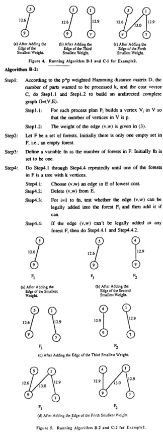
Algorithm 0-2:

Stepl: According to the p*p weighted Hamming distance matrix D, the number of parts wanted to be processed k, and the cost vector C, do Stepl.1 and Stepl.2 to build an undirected complete graph G=(V.E).

Stepl.1: For each process plan Pi builds a vertex Vi in V so

that the number of vertices in

V

is p. Stepl.2: The weight of the edge (v,w) is given in (3). Let F be a set of forests. Initially there is only one empty set in

F,

i.e., an empty forest.

De& a variable fn as the number of forests in F. Initially fn is set to be one.

Do Step4.1 through Step4.4 repeatedly until one of the forests in F is a tree with k vertices.

Step4.1: Choose (v.w) an edge in E of lowest cost. step4.2: Delete (v.w) from

E.

Step4.3: For i=l to fn, test whether the edge (v,w) can be legally added into the forest Fi and then add it if Step2:

Step3:

Step4:

Can.

Step4.4 If the edge (v,w) can't be legally added in any forest Fi then do Step4.4. I and Step4.4.2.

(a) After Adding the Edge Of IhC S d C S t

Weight

(b) After Adding thc Edge ofthe Second

Smalles~ Wcighhr

F1 F2

(c) After Adding the Edge of the Third SmaUesl Weight.

F1 F2

(d) After AddinL Ihc Edge ofthc F m h Smallerl \\'eight.

(5)

Step4.4.I: Step4.4.2:

fn t fn

+

I.

Clear the forest Fh to be empty, and,

then, add the edge (v,w) into this new forest.

Now there is at least one forest F, in F become a tree with k

vertices. If there exists more than one such trees in F then find

a tree F,,,, with smallest cost according to the cost function (1). Then the set of process plans represented by the corresponding vertices in F,, is a valid selection for processing the total k Parts.

Steps:

The major difference between algorithm B-2 and B-1 is that F in algorithm B-2 is a set of forests instead of a set of trees, and a new forest Fmcl with a single edge (v,w) must be constructed if the edge (v,w) can't be legally added into any forest Fi, I l i l f n . For illustration figure 5 shows the forests built by algorithm B-2 for example 2. Figure 5(b) shows that the second smallest edge (v4, vg) can't be legally added into the forest FI and, hence, a new forest F2 is then constructed. In figure 5(c) the third smallest edge (v1,v7) can be legally added into both Fl and F2 so that it is incorporated into both of them. At last, there are two spanning trees, F, and F2, with four vertices as shown in figure 5(d). After the total cost of these two trees is calculated, the set of process plans (P1,P4,P7P9} is the final solution which is also the optimal solution.

C. Process Plan Sequencing Problem

The necessary information for this problem is the same as the above one, i.e., a weighted Hamming distance matrix D, a variable k

indicating the number of parts wanted to be processed, and a cost vector C. The algorithms for solving this problem are similar to that for solving the previous problem except that the testing procedure is different and the weight in every edge when building the corresponding graph G is also different. Specifically, the weight for the edge (v,w) is defined as the sum of C,, C,,,,

and

2 * 4 , in view of the fact that the total weight of edges in a sequence is twice of that given by (2) according to this weight definition. Furthermore, when the edge (v,w) is chosen, we must test after it is added whether the forest can form a valid sequence instead of whether it can form a valid spanning tree. Two algorithms for solving this class of problems are shown as follows.

Algorithm C-1: Step I :

Step2:

Step3:

Step4:

According to the pxp weighted Hamming distance matrix D, the number of parts to be processed k, and the cost vector C, do Stepl.1 and Stepl.2 to build an undirected complete graph W V , E ) .

Stepl.1: For each process plan P, builds a vertex Vi in V so that the number of vertices in V is p.

The weight of edge (v,w) is the sum of C,, C,, and 2*4.w.

Stepl.2:

Let F be a set of trees, that is, a forest. Initially, F is an empty set with no element.

Do Step3.1 through Step3.3 repeatedly until F becomes a sequence with k vertices.

Step3.1:

Step3.2: Delete (v,w) from E.

Step3.3: Test whether the edge (v.w) can be legally added into forest F and then add it if can.

Now the forest F contains only one sequence S. This implies that the order of process plans represented by the corresponding vertices in S is a valid sequence for processing the total k parts.

Choose (v,w) an edge in E of lowest cost.

Algorithm C-2: Stepl:

Step2

Step3:

Step4:

According to the pxp weighted Hamming distance matrix D, the number of parts to be processed k, and the cost vector C, do Stepl.1 and Stepl.2 to build an undirected complete graph G=(V,E).

Stepl.1: For each process plan Pi builds a vertex V i in V so that the number of vertices in V is p.

Stepl.2: The weight of edge (v,w) is the sum of C,, C,, and

Let F be a set of forests. Initially, there is only one empty set in F which indicates that there is an empty forest in F at first. Define a variable fn as the number of forests in F. Initially ti^ is set to one.

Do Step4.1 through Step4.4 repeatedly until there is a forest Fi in F being a valid sequence with k vertices.

Step4.1: 2* 4.w

Choose (v,w), an edge in E of lowest weight.

(40.8) 0.1123 0.1697 40.032 0 % 2 % 16.85% 14.11% SI.OR% 2.314%

(40.10) 0.1233 0.3887 56.152 0% 0 % 13.81% 9.82% 215.1% 3.528% (50.10) 0.1967 0.4231 803.43 0 % 0 % 16.18 % 13.14 % 174.4 % 2.512 'b

(50.12) 0.2217 0.7082 1261.6 0 % 0 % 14.53 % 10.11 % 219.3 % 3.695 %

run time : CPU run time (sec) on VAX 8530 OPT': exhaustive mehod for finding optimal roluiion.

DRATIO' : diflercncc ratio hhveen approximate solution and optimal solution.

Tahle 5. Fcrlormance of Algorllhm D-1 and D-1. (avcrapc value lor 50 inslanccs each problem solved)

(6)

Steps: sin: (p.W Step4.2: Delete (v.w) h m E. Step4.3: Step4.4:

For i=l to ti, test whether the edge (v,w) can be legally added in forest Fi and then add it if can. If the edge (v.w) can't be legally added in any forest Fi then do Step4.4.1 and Step4.4.2. Step4.4.1: fn c fn

+

1.

Step4.4.2: Clear the forest F, to be empty then add (v.w) in this new forest. Now there is at least one forest Fi in F become a valid sequence with k vertices. If there exists more than one such sequences in F then find a tree Fmi, with the smallest cost according to the cost function (2). Then the sequence of process plans repmented by the corresponding vettices in Fmin is a valid one for processing the total k parts.

DRATIO@ nlio or finding oplimal snlulion computer mn lime c-2

I

O F r

I

c-l

I

c-2

I

c-l

I

c-2 c-l

1

For example, after the edge (vI,v4) is added into the forest shown in figure 61a) the forest in figure 6(b) is not 3 valid sequence although it is a valid tree. Application of these two algorithms to example 2 are shown in figure 4 and figure 5 respectively. Then forests built by these algorithms are found to be the same as the ones built by algorithm B-1

and B-2 because the weights C;/(4-1) (used in algorithm B-1 and 8-2)

are equal to 2 (use in algorithms C-1 and C-2). In figure 4 the process sequence obtained is P+P9+P,+P7 (or P7-+P,+P9+P5) which is the optimal solution. In figure 5(d) two valid sequences are obtained. After their respective costs are calculated, the final solution is the same as the above one.

IV. Computer Simulation Examples

In this section, we implement some simulation programs of the algorithm B-I, B-2, C-I, and C-2 on VAX 8530 to solve the relevant problems. Comparison between results of our approachs and the optimal solutions is performed and shown. In order to analyze the performance of these algorithms, random problems of various sizes (p,k) were generated. Here p is the number of process plans

and

k is the total number of parts. The cost C,, for each 1 4 5 ~ . were uniform in interval (0,15) and the Hamming distances were random integers in [1,10]. Table 5 and 6 sum- marize the results obtained.

The first column of table 5 shows the computer run time of three algorithms: B-I. B-2, and a exhaustive search method to find the optimal solution (say, OPT method). Since the process plan selection is NP- complete, the run time of OPT method grows greatly as the problem size increases. The result shows that algorithm B-1 and B-2 are both very efficient because of the little run time. The second column demonstrates the percent of finding the optimal solution of algorithm B-1 and B-2. It is shown that it will become more and more difficult to find the optimal solution for these methods as the problem size increases. The third column lists the difference ratio between the optimal solution and that

(a) Oribinal Forest. (b) An h a l i d S q w n c c .

Figure 6. Example of an I n l a l i d Sequence.

run tim : Cmr mn lime (SE) on VAX 8530. om' : clhaustire method lor finding optimal solution

DRATIO" : differma nlio b e l m n approximate solution and optimal solution.

Tahle 6. Pcrrormanca or Algorithm C-1 and C-L

(average value lor IO Instances each problem solved)

our approach found. The result shows that the value obtained from algorithm B-2 is about ten to fourteen percent off the value of best solution, and the solution obtained kom algorithm B-1 is a little worse than that from algorithm B-I. The last column reveals that the improvement of solution quality is about 2 to 6 percent of algorithm B-2, but the computer time needed is much longer than that of algorithm B-1 as the problem size increases. Finally it seems to make the application of algorithm B-2 worthwhile.

The similar results are shown in table 6 for algorithm C-1 and C-2.

To sum up, we can see that algorithm C-1 is a very efficient and satisfactory method when applied to the process plan sequencing problem.

V. Conclusion

An efficient method of solving problems of classification and selec- tion using minimum spanning tree in an FMS is proposed in this paper. Computer simulation examples anthen provided which shows a satisfactory result. Especially, the total computational time spent is also econom- ical. The application of this method to these classes of problems will be quite promising. Ongoing research will be on considering the very flexibility nature of an M S

and

then extending this method to solve more dynamic and general problems in an M S .

VI. Reference

1. Ham, K. Hitomi, and T. Yoshida, Group Technology, Kluwer Nijhoff publishers, Hingham, Mass., 1985.

C. C. Gallagher and W. A. Knight, Group Technology. Butterworth & Company (Publishers) Ltd., London, 1973.

A. Kusiak, A. Vaonelli, and K. R. Kumar, "Grouping problem in scheduling flexible manufacturing systems," Robotica, vol. 3, pp. 245-252, 1985.

J. B. KNskal, "On the shortest spanning subtree of a graph and the traveling salesman problem," in Proc. h e r . Math.. S o c . 7:1, 48-

so.

T.

C. Chang and R. Wysk. An Introduction to Automated Process Planning Systems, Englewood Cliffs, HJ: F'rentic-Hall, 1985. A. Kusiak and G. Finke, "Selection of process plans in automated manufacturing systems,'' IEEE J. of R . and A., vol. 4, no. 4, Aug. pp. 397-402, 1988.