國立交通大學
電信工程學系
碩士論文
以虛擬基地台為輔助的無線位置估測
Wireless Location Estimation with the Assistance
of the Virtual Base Stations
研究生:陳建華
指導教授:方凱田
以虛擬基地台為輔助的無線位置估測
Wireless Location Estimation with the Assistance of Virtual Base Stations
研究生:陳建華
Student:Chien-Hua Chen
指導教授:方凱田
Advisor:Kai-Ten Feng
國立交通大學
電信工程學系碩士班
碩士論文
A Thesis
Submitted to Department of Communication Engineering
College of Electrical and Computer Engineering
National Chiao Tung University
in Partial Fulfillment of the Requirements
for the Degree of
Master of Science
in Communication Engineering
June 2006
以虛擬基地台為輔助的無線位置估測
學生:陳建華 指導教授:方凱田
國立交通大學電信工程學系碩士班
摘要
隨著商業應用的潮流,無線位置估測的技術在近年來被廣泛的研究著。很多種形式
的無線訊號都可以作為位置估測之用。在這篇論文之中,由傳播時間轉換過來的量
測距離首先被線性化,以便利用最小平方 (Least Square) 估計的方法。論文裡考
量兩個實務上的問題,分別是〝非直接路徑 (NLOS) 誤差〞與〝幾何衰減 (GDOP) 效
應〞
。在量測時間資訊時,非直接路徑誤差會引發ㄧ個正值而且很大的偏差。另ㄧ方
面,基地台的幾何分佈不佳時,幾何衰減效應的值會增加,進而降低定位的準確度。
這篇論文所提出的〝虛擬基地台 (VBS) 輔助演算法〞藉由加入一些幾何限制以降低
非直接路徑誤差的影響;也藉由加入一些虛擬基地台來減少幾何衰減效應。所提出
的虛擬基地台輔助演算法在模擬時與一些現有的定位演算法相比較。模擬結果顯示
虛擬基地台輔助演算法的表現較好,特別是在非直接路徑誤差很大與基地台幾何位
置不佳時的錯誤率表現更佳。
國立交通大學
電信工程學系
碩士論文
以虛擬基地台為輔助的無線位置估測
Wireless Location Estimation with the Assistance
of the Virtual Base Stations
研究生:陳建華
指導教授:方凱田
以虛擬基地台為輔助的無線位置估測
Wireless Location Estimation with the Assistance of Virtual Base Stations
研究生:陳建華
Student:Chien-Hua Chen
指導教授:方凱田
Advisor:Kai-Ten Feng
國立交通大學
電信工程學系碩士班
碩士論文
A Thesis
Submitted to Department of Communication Engineering
College of Electrical and Computer Engineering
National Chiao Tung University
in Partial Fulfillment of the Requirements
for the Degree of
Master of Science
in Communication Engineering
June 2006
Wireless Location Estimation with the Assistance of Virtual Base Stations
Student:Chien-Hua Chen Advisor:Kai-Ten Feng
Department of Communication Engineering
National Chiao Tung University
Abstract
The wireless location estimation techniques have been wildly investigated with
the trend of commercial applications in recent years. Various types of radio
signals can be used to develop the location estimation algorithms. In this thesis,
the range measurements transferred from the received time-based information
are first linearized to utilize the Least Square (LS) method. The practical issues
such as the Non-Line-of-Sight (NLOS) errors and the Geometric-Dilution-of-
Precision (GDOP) effect are concerned. The NLOS errors will cause a large
positive bias while measuring the time information. On the other hand, the poor
geometric layout will raise the GDOP value and reduce the accuracy of a location
algorithm. The proposed VBS (Virtual Base Stations) algorithm mitigates the
influence of the NLOS errors by adding some geometric constraints and reduces
the GDOP effect by joining the assisted virtual base stations. The proposed VBS
algorithm is compared with several existing location algorithms via simulations.
The performance is comparably better than other methods, especially in the
environments with large NLOS errors and poor geometric layout.
致 謝
很感謝指導教授方凱田老師讓我進入了這個充滿活力、淺力無窮的實驗室。
在研究的路上,很感謝老師給我發揮的空間,讓我作ㄧ些有興趣的議題。在人生
規劃上,也很感謝老師與我作經驗分享,讓我可以自信地向前邁進。也感謝口試
時,給予寶貴建議的交大電信吳文榕教授和交大資工王國禎教授;有了這些建議
和問題,更能使我的研究愈臻周全和完整。
在來到交大電信所之後,我很幸運地和智迪、名宇、中義、冠宏與偉祥成為
朝夕相處的同學。我們一起作研究,一起讀書,一起遊玩;透過他們,我認識了
更多同學和朋友。大家的感情都很好,這是我的碩士求學期間的重要收穫。我想
謝謝他們大家,因為他們豐富了我碩士時期的時光。
在專業的研究上,每周長達三小時和老師、壆長昭霖、學弟柏軒與育群的討
論對我的研究有很大的幫助。學長昭霖給與的建議和指教,使我的研究更紮實;
學弟柏軒與育群的另類思考,也讓我激發出更多有趣的想法。每次都在熱烈討論
的小組會議之後,拖著疲憊的身體回寢,但是腦海中那些大家集思廣益的想法,
正是使研究更加前進的動力。就在一次又一次的努力和嚐試之後,我承繼著實驗
室之前的研究而完成了一個完整了演算法,也算是對自己碩士班研究成果的一個
呈現。
我要特別感謝我的妻子謝瑩穎。撰寫碩士論文期間的苦悶和趕稿的壓力真的
讓人很疲累。瑩穎給我充分的時間,讓我能專心的完成我的論文,同時也不斷的
鼓勵我,讓我在愈益疲憊的身心下還能打起精神繼續努力。我很感謝她為我所做
的一切。最後,我要感謝我的父母和岳父母,謝謝他們的支持和鼓勵。我要將我
的小小成果歸功於我的阿嬤、父母、岳父母和我最愛的妻子。
陳建華謹誌 於新竹交通大學
Contents
1 Introduction 5
2 Related Work 8
2.1 Mathematical Modeling . . . 8
2.2 Studies on Existing Location Estimation Algorithms . . . 9
2.2.1 The Subspace Method . . . 9
2.2.2 The Beamforming Method . . . 11
2.2.3 The Fingerprinting Method . . . 11
2.2.4 The Ray-Optical Approach . . . 12
2.2.5 The Taylor-Series Estimation (TSE) Algorithm . . . 14
2.2.6 The Two-Step Least Square (two-step LS) Algorithm . . . 16
2.2.7 The Linear Line-of-Position (LLOP) Method . . . 19
2.3 Studies on Propagation Noise . . . 22
2.3.1 Overview . . . 22
2.3.2 Methods Proposed to Mitigate or Reduce the NLOS error . . . 23
2.4 Studies on an Important Metric — Geometric Dilution of Precision (GDOP) . 33 3 The Location Estimation with The Assistance of Virtual Base Stations 35 3.1 Overview . . . 35
3.2 Observations from the GDOP . . . 37
3.3 The Extended Two-Step LS Algorithm with Virtual Base Stations . . . 40
3.3.2 Formulation of the Extended Two-Step LS Algorithm . . . 41
3.4 The Selection of a Virtual Base Station . . . 44
3.4.1 The Center of Gravity (CG) Based Selection Method . . . 44
3.4.2 The Minimum GDOP (MG) Based Selection method . . . 45
4 Performance Evaluation 48 4.1 The Noise Models and Simulation Parameters . . . 48
4.2 Simulation Results . . . 49
List of Figures
1.1 Position Determination Methods: (a) Time of Arrival (b)Time Difference of
Arrival (c) Angel of Arrival . . . 6
2.1 Geometric Description of Three-Antenna Case . . . 10
2.2 The Ray-Optical Approaches Include (a) the Ray-Tracing Method and (b) the Ray-Launching Method . . . 13
2.3 The Geometry of TOA-Based Location with Circular LOPs and Linear LOPs . 20 2.4 The Range Measurements Suffer from the NOLS Errors. . . 23
2.5 The Flow Chart of the Rwgh Algorithm . . . 24
2.6 Mobile location estimation using the Kalman Filtering . . . 27
2.7 The Geometry of the TOA-Based Location Showing the Relationship of the True Ranges and Inter-BS Distance. . . 28
2.8 Geometric Constraints for TOA-Based Location Estimation Confine the True MS’s Position in the Overlap Region of the Range Measurements. . . 29
3.1 The Flow Chart of the VBS Algorithm . . . 36
3.2 The GDOP Value in a Regular Triangle. . . 38
3.3 The GDOP Value in a Square. . . 38
3.4 The GDOP Value in a Regular Pentagon. . . 39
3.5 The GDOP Value in a Regular Hexagon. . . 39
4.1 Performance Comparison between the Location Estimation Schemes under NLOS Environments in Case(1) (with Median Value of the NLOS Noises: τm=0.3 µs) . . . 50
4.2 The Positioning Processes of the VBS Schemes under NLOS Environments in Case(1) (with Median Value of the NLOS Noises: τm =0.3 µs) . . . 51
4.3 Performance Comparison between the Location Estimation Schemes under NLOS Environments in Case(2) (with Median Value of the NLOS Noises: τm=0.3 µs) . . . 51
4.4 The Positioning Processes of the VBS Schemes under NLOS Environments in Case(2) (with Median Value of the NLOS Noises: τm =0.3 µs) . . . 52 4.5 Performance Comparison between the Location Estimation Schemes under
NLOS Environments in Case(3) (with Median Value of the NLOS Noises: τm=0.3 µs) . . . 53
4.6 The Positioning Processes of the VBS Schemes under NLOS Environments in Case(3) (with Median Value of the NLOS Noises: τm =0.3 µs) . . . 53
4.7 Performance Comparison between the Location Estimation Schemes under NLOS Environments in Case(4) (with Median Value of the NLOS Noises: τm=0.3 µs) . . . 54 4.8 The Positioning Processes of the VBS Schemes under NLOS Environments in
Case(4) (with Median Value of the NLOS Noises: τm =0.3 µs) . . . 54
4.9 The Comparison of the 60% Average Position Errors of the Location Estimation Methods under Different NLOS Errors . . . 55
Chapter 1
Introduction
Wireless positioning techniques have been wildly studied over the past few decades. Today, more and more commercial applications such as the navigation system, the location-based billing, and the Intelligent Transportation System (ITS) need to cooperate their own processes with the information from the positioning systems. After the issue of the emergency 911 (E-911) subscriber safety service, the QoS of the positioning accuracy has been first-time defined. The importance and the requirements of the positioning techniques in many fields excite the research in this domain. Because of such interests and demands in location-based services (LBSs) , the studies of a new location estimation scheme considers different environment properties has been carried out.
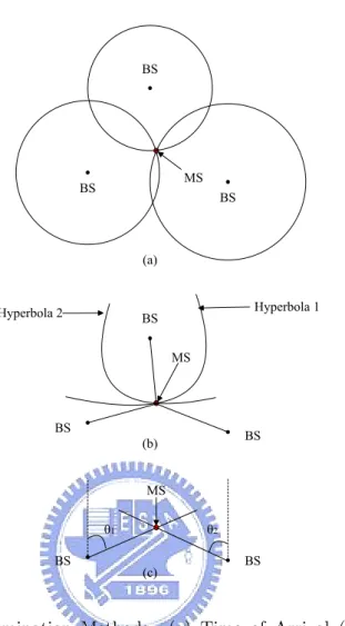
The time-based information, said the Time-of-Arrival (TOA), is directly proportional to the distance between the transmitter (i.e. Mobile Station or MS) and the receiver (i.e. Base Station or BS). With simply multiplying by the speed of light, the distance above can be easily obtained. As presented in Fig. 1.1.(a), a range circle with a receiver being the center and the corresponding measured distance being the radius can be obtained from each communication channel. Evidently, every single point on such a circle represents a possible location of the wanted MS. The circles of two different base stations (BSs) will intersect at two points without considering the special cases of tangency and non-intersection. Three range circles are the least information required to acquire an unique point. This result can be applied to the
BS BS (a) (b) BS BS BS (c) θ1 θ2 BS Hyperbola 1 Hyperbola 2 BS BS MS MS MS
Figure 1.1: Position Determination Methods: (a) Time of Arrival (b)Time Difference of Arrival (c) Angel of Arrival
satellite-based and the network-based location schemes which are two major categories in existing wireless location systems.
The concept of time difference can also be used to solve the problem of positioning in the network-based system. Since the propagation time and distance between each pair of a BS and an MS are closely related, the difference of two measured time information can be associated with that of two measured distances in thinking. A hyperbola curve with two BSs as the foci can be introduced from the formulation of the difference of two distances. The intersection of two hyperbola curves will be viewed as the position of the MS, as shown in Fig. 1.1.(b). Hence the information of the Time-Difference-of-Arrival (TDOA) can be transformed
into a geometric relationship and applied in the application of positioning. The extra demand in the network-based system utilizing the TDOA scheme is that synchronization of the BSs is necessary.
In a two-dimensional (2-D) scenario, an object can be localized with hybrid time and/or angle information. The Angle-of-Arrival (AOA) , also known as the Direction-of-Arrival (DOA) , can be adopted to proceed the task of positioning. On a reference coordinates, a line from a BS to the MS can produce an angle. It requires at least two lines that intersect with each other to locate the MS in the AOA scheme as shown in Fig. 1.1.(c). With the uncertainty of the position of MS, antenna arrays or multi-dimensional antenna are needed for every BS to obtain the direction.
The TOA, TDOA and AOA information mentioned above can be utilized individually or can be cooperated with each other in a network-based location estimation system [1] [2]. Since the expression of the distance contains inherently nonlinear terms, many mathematical solutions can not be adopted to solve the problem. Therefore, linearized approaches are applied to re-formulate the expression and estimate the position of MS [3]. However, one thing to be emphasized is that only the Line-of-Sight (LOS) case is concerned in these location methods. In this thesis, more realistic noise and interference are considered. A VBS scheme is proposed to estimate the location of MS under the considerations of NLOS (Non-Lone-of-Sight) and GDOP (Geometric-Dilution-of-Precision).
The remainder of this thesis is organized as follows. The related work, including the mathematical modeling, the existing location estimation algorithms, the propagation noise, and the GDOP effect, is briefly described in chapter 2. The observation from GDOP and the formulation of the VBS algorithm are discussed in chapter 3. The performance evaluations are shown in chapter 4, followed by the conclusions remark in chapter 5. The reference is outlined in the last part.
Chapter 2
Related Work
2.1
Mathematical Modeling
The mathematical models for the TOA, TDOA, and AOA measurements are summarized as follows. The TOA measurement t` from the `th BS is obtained by
t`= rc` = 1cζ`+ n` ` = 1, 2, ...n (2.1)
where c is the speed of light, and r` represents the measured relative distance between the MS and the `th BS contaminated with the TOA measurement noise n
`. The noiseless relative
distance ζ` between the MS and the `th BS can be obtained as
ζ` = kx − x`k (2.2)
where x = (x, y) represents the MS’s position, and x` = (x`, y`) is the location of the `th
BS in the 2-D setting; while in the 3-D formulation, x = (x, y, z) and x` = (x`, y`, z`). On
the other hand, the TDOA measurement ti,j is obtained by computing the time difference
between the MS w.r.t. the ith and the jth BSs as:
where ni and nj represent the measurement noises from the MS to the ith and the jth BSs.
Since it is assumed that the antenna arrays at the home BS can only measure the incoming signals along the x and y directions, the AOA measurement θ of the cellular system is obtained as
θ = tan−1(y − y1 x − x1
) + nθ (2.4)
where θ represents the horizontal angle between the MS and its home BS. (x1, y1) is the
horizontal coordinate of the home BS, and nθ is the measurement noise associated with θ.
2.2
Studies on Existing Location Estimation Algorithms
Different location estimation schemes have been proposed to acquire the MS’s position. Various types of information (e.g. the signal propagation time, the received angle of the signal, or the Receiving Signal Strength (RSS)) are involved to facilitated the algorithms design for location estimation. The primary objectives in most of the location estimation algorithms are to obtain higher estimation accuracy with promoted computational efficiency.
2.2.1 The Subspace Method
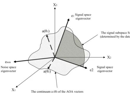
The subspace method is also known as the super-resolution method or the high-resolution method. The multiple radio wave fronts or the superposition of them are received by sensor arrays at a receiver. It utilizes the eigendecomposition or the eigenanalysis process of the cross-correlation matrix to generate the estimates of some particular parameters contained in the signals. These parameters can be the number of signals, the AOA information, the signal strength, the noise strength or the characteristic (like gain, phase and polarization) of the an-tennas. The most well-known super-resolution algorithm is the MUltiple SIgnal Classification (MUSIC), which can be implemented as an unbiased estimator asymptotically. The MUSIC scheme studied in [4] considers arbitrary-located antennas and a particular covariance matrix within a noisy environment.
X1 X3 X2 e1 e2 emin a(θ1) a(θ2) Signal space eigenvector Signal space eigenvector Noise space eigenvector
The signal subspace Ss (determined by the data)
The continuum a (θ) of the AOA vectors (determined by array geometry and characteristic)
Figure 2.1: Geometric Description of Three-Antenna Case
As shown in Fig. 2.1, multiple transmitted signal wavefronts arrival with varies directions. The incident signal vectors a(θ1) and a(θ2) can construct the range space a. The vectors E1,
E2 and E3 are the eigenvectors of the covariance matrix S of the received vector r. The λ1,
λ2 and λ3 are the corresponding eigenvalues and λ1 > λ2 > λ3 > 0. The signal subspace Ss
can be generated by the vectors E1and E2 while the vector E3 can form the noise space. The
received vector r can be represented as the linear combination of the vector E1, E2 and E3.
The AOA parameter can be solved by intersecting the vector a and the signal subspace Ss.
The MUSIC scheme is experimentally illustrated to be a robust solution for location estimation, especially for a near-far environment. Over fading channels, the estimator in [5] applying the MUSIC identification method intents to estimate the propagation delay of the received signal in a DS-CDMA system. In [6], the variance of the MUSIC signal source location estimates is derived and the synthetic formulation can be adopted to the correlation matrix of a biased estimator. However, it has also be shown in [7] and [8] that the drawbacks of the MUSIC approach include (i) comparably high sensitivity to large noise and (ii) its complexity in computation.
2.2.2 The Beamforming Method
The beamforming system is a space-time processor that operates on the output of sensor arrays. The received temporal signal with spatial wavefront being a function of its unknown MS’s position can be proceeded to locate multiple MSs, restrain interferences, and mitigate noise. It supports spatial filtering capability by enhancing the amplitude of a coherent signal associated with surrounding noises. The conventional adaptive beamforming technique is sensitive to the estimation error of the position of MS. Signal distortion or cancellation will be introduced in the iterative process.
A combination of localization and beamforming is proposed as in [9]. It utilizing the MU-SIC scheme to provide the ability of self-correcting and increase the robustness to locate errors without sacrificing the computation efficiency under the assumption that the number of MS and the characteristic of the noise are known. An enhanced algorithm for simultaneous multi-source beamforming and adaptive multi-target tracking is studied in [10]. The correlation between the adaptive minimum variance (MV) beamforming and the optimal source localiza-tion is also investigated and developed as in [11]. Under equal priors, it shows that the optimal source localization decision rule (i.e. the log-likelihood function) is directly proportional to the output power of the adaptive MV beamformer.
2.2.3 The Fingerprinting Method
Instead of exploiting the spatial and temporal information of the signal, the location fingerprinting technique locates the MS based on the received signal strength (RSS) .
The fingerprinting technique involves both the off-line and the on-line phases. First in the off-line mode, the location fingerprinting senses the RSS from multiple access points (AP) in a 802.11 wireless local area network. A location-scanned database is stored in a sink node and a rectangular grid network covered a specific service area is ready as a radio map after collecting enough statistical data. The location fingerprinting means the signal strength value at a grid point of the radio map. The second mode comes with the on-line phase in real-time processes. When a radio signal is received at multiple access points, a measured RSS vector can be
obtained and is used to compare with the location fingerprinting map at the sink node. In order to minimize the error of location estimation, it generally applies a proximity-matching method, like Euclidean distance, to figure out the position of the MS.
The characteristics of radio signals in indoor environments are discussed in [12]. For WLAN location fingerprinting, the distribution of RSS is usually not Gaussian, and its stan-dard deviation is signal-level dependent. In addition, it demonstrates that the effect of the existence or movement of persons apparently affects the location fingerprinting and the infor-mation of the changes should be recorded on the sink node. In [13], a method for arranging and designing parameters is proposed when considering deploying a indoor positioning sys-tem. A hybrid algorithm, which combines the RF propagation loss model, is proposed to both mitigate the requirement of the training data and to adjust the configuration changes [14].
2.2.4 The Ray-Optical Approach
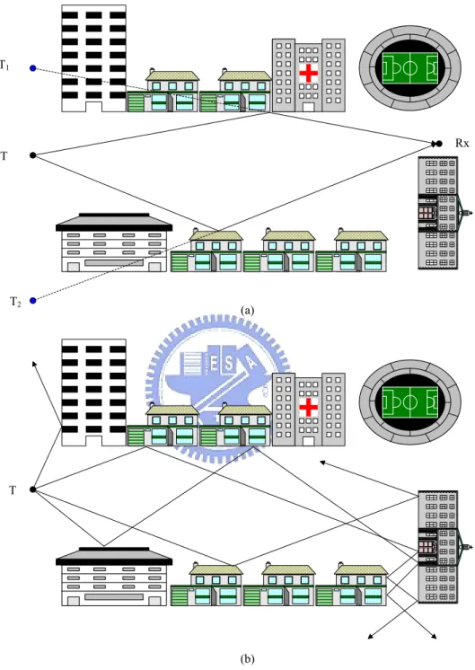
The ray-tracing and ray-launching techniques are the two ray optical approaches for lo-cation estimation. The radio signals that are launched from a transmitter and reflected or diffracted by various objects are aggregated in a receiver. The rays are treated as the traces of radio signals and are summed individually to determine the corresponding electric field strengths.
In the method of ray-tracing, the generation of a image comes with a reflection of a ray. As shown in Fig. 2.2.(a), the images T1 and T2 are relative to the transmitter T. High accuracy can be achieved by tracking each trace apart, but the cost of high computation time can not avoid. In the ray-launching approach, as illustrated in Fig. 2.2.(b), rays launched from the transmitter reflect and diffract across the indoor circumstance. Every time a ray reflect from a wall or diffract by a cone, the number of intersections will be added by 1 and the field will be accumulated. When the number of intersection or path loss exceed a threshold, the tracing of a ray will stop. One thing to be emphasized is that a vast amount of diffracted rays may be introduced and heavily increase the load of the location system.
T1 T2 T Rx (a) T (b)
Figure 2.2: The Ray-Optical Approaches Include (a) the Ray-Tracing Method and (b) the Ray-Launching Method
losses are studied as in [15] [16]. The unknown indoor parameters, such as materials, layouts will significantly affect the propagation predictions of rays. An indoor micro cell area pre-diction system is proposed in [17] and the prepre-diction can be effortlessly estimated by using ray-tracing scheme.
A ray-launching approach is enhanced with two methods, i.e. the effective-propagation-area method and the dominant-corner extraction method [18]. By restricting the behaviors of the propagations, it saves the computation time and efficiently fulfills the prediction of prop-agation characteristics. The improved three dimensional indoor radio propprop-agation techniques are developed in [19] and [20].
2.2.5 The Taylor-Series Estimation (TSE) Algorithm
In [21], the Taylor series method is applied to linearize the equations of the range mea-surements and hence the location calculations are simplified.
As mentioned in section 2.1, (x, y) is the position of the MS and (x`, y`) is the position of the `th base station and r
` is the TOA measurement from the base station `. Assuming that
the propagation noise can be neglected, the range measurement can be expressed as
ζ` = r`− n` = f`(x, y, x`, y`) (2.5)
where ζ` represents the noiseless distance between the MS and the `th BS. n
` is the
mea-surement noise and is statistically distributed. We take the noises to have zero-mean values < n`>=0 and nij =< ninj > is the i − jth term in the covariance matrix
Q = [nij]
If the xv, yv are the initial guessed values of the true MS’s position, the MS’s position (x,y)
can be written as
where δx and δy are the deviations of the MS’s position (x, y) and the corresponding initial guessed position (xv, yv).
Expand the function f` in Taylor’s series by keeping only terms below second order as:
f`= r`− n` ∼= f`v+ a`1δx+ a`2δy (2.7)
where
f`v = f`(xv, yv, x`, y`)
a`1= ∂f`/∂x|xv,yv a`2= ∂f`/∂y|xv,yv
The approximate relations of (2.7) can be written as
Aδ ∼= z − n (2.8) where A = a11 a12 a21 a22 . . aN 1 aN 2 δ = δx δy z = r1− f1v r2− f2v . rN − fN v n = n1 n2 . nN
The parameter δ can be chosen as
δ = (ATQ−1A)−1ATQz (2.9)
Thus, to estimate the position of the MS, compute δx, δy with (2.9), replace
xv ← xv+ δx yv ← yv+ δy (2.10)
essentially zero.
2.2.6 The Two-Step Least Square (two-step LS) Algorithm
The content of this section will show the two-step least square location algorithm for the TOA measurements and it can be obtained in [22]. The two-step LS method for the TDOA measurements can be derived from the similar concept.
The notations of the MS’s position and the base stations are the same as those in the TSE algorithm described in the previous section. The small propagation noises are concerned in the two-step LS algorithm. The additive noises are assumed to be Gaussian-distributed and independent of the radio signals. By incorporating the influences of the propagation errors on the location estimation, the range measurements can be formulated as
r2` ≥ (x`− x)2+ (y`− y)2 = κ`− 2x`x − y`y + x2+ y2 ` = 1, 2, ...N (2.11)
where κ` = x2`+y2`, r`= ct`is the measured distance between the MS and the `thbase station,
and c is the speed of light. And by defining a new variable β = x2+ y2, we rewrite (2.11) through a set of linear expressions
−2x`x − 2y`y + β ≤ r2` − κ` ` = 1, 2, ...N (2.12)
Let xa= [x y β]T and express (2.12) in matrix form
Hxa≤ J (2.13) where H = −2x1 − 2y1 1 −2x2 − 2y2 1 . . . −2xN − 2yN 1 J = r2 1− κ1 r2 2− κ2 . r2 N− κN
With measurement noise, the error vector is
ψ = J − Hxa (2.14)
When r` can be expressed as ξ`+ cn`, the error vector ψ is found to be
ψ = 2cBn + c2n ¯ n
B = diag{ξ1, ξ2, ..., ξN} (2.15)
The symbol ¯ represents the Schur product (element-by-element product). In addition, the second term on the right of (2.15) can be ignored since the condition cn` ≤ ξ` is usually
satisfied. As a result, ψ becomes a Gaussian random vector with covariance matrix given by
Ψ = E[ψψT] = 4c2BQB (2.16)
Q is the covariance matrix of measured noise, and ξ1,...,ξN are denoted as the true values of distances between the sources and the receiver. The element xa are related by the equation,
β = x2 + y2, which means that (2.13) is still a set of nonlinear equations in two variables
x and y. The approach to solve the nonlinear problem is to first assume that there is no relationship among x, y and β. It can then be solved by the Least Square (LS) method. The final solution is obtained by imposing the known relationship to the computed result via another LS computation. This two step procedure is an approximation of a true Maximum Likelihood (ML) estimator. By considering the elements of xaindependent, the ML estimator
of xa is
xa = arg min{(J − Hx )TΨ−1(J − Hx )}
= (HTΨ−1H)−1HTΨ−1J (2.17)
(2.17). The covariance matrix of xa can be calculated as [23]
cov(xa) = (HTΨ−1H)−1 (2.18)
Since we have used the independent supposition of variables x, y, and β in the estimation of xathough the variable β is dependent on the variable x and y, we should revise the results
as follows. Let the estimation errors of x, y, and β be e1, e2, and e3. Here and below, denote
the ith entry of a matrix M as [M ]
i; then the entries in vector xa become
[xa]1 = xo+ e1 (2.19a) [xa]2 = yo+ e2 (2.19b)
[xa]3 = βo+ e3 (2.19c)
where xo, yo, and βo are denoted as the true values of x, y, and β. Let another error vector
ψb = Jb− Hbxb (2.20) where Hb= 1 0 0 1 1 1 Jb= [xa]21 [xa]22 [xa]3 and xb= x 2 y2
. Substituting (2.19a) - (2.19c) into (2.20), we have
[ψ]1 = 2xoe1+ e21 ≈ 2xoe1
[ψ]2 = 2yoe2+ e22≈ 2yoe2
[ψ]3 = e3
small. Subsequently, the covariance matrix of ψb is
Ψb = E[ψbψTb] = 4Bbcov(x )Bb
Bb = diag{xo, yo, 0.5} (2.22)
As an approximation, elements xoand yoin matrix x can be replaced by the first two elements
x and y in xa. Similarly, the ML estimate of xb is given by
xb = (HTbΨ−1b Hb)−1HTbΨ−1b Jb (2.23)
≈ (HTbB−1b (cov(x )a)−1B−1b Hb)−1 (2.24) • (HTbB−1b (cov(x )a)−1B−1b )Jb (2.25)
So the final position estimation x = [x y]T is
x =√xb, or x = −
√
xb (2.26)
Here the sign of x should coincide with the sign of [xa]1 calculated by solving (2.17), and the
sign of y coincides with the sign of [xa]2.
The complete derivation of the the two-step LS for the TOA measurements is shown as above. In addition, the two-step LS method can be adopted to estimate MS location from the TDOA [23], and the TDOA/AOA measurements [24].
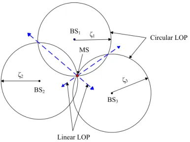
2.2.7 The Linear Line-of-Position (LLOP) Method
The linear line-of-position methods can be utilized to locate the MS’s position by using the TOA measurements as in [25], and the hybrid TOA/AOA measurements in [26]. The content of this section will show the linear Line-of-Position (LLOP) and it can be referred to [25].
BS1 BS2 BS3 ζ1 ζ2 ζ3 Linear LOP Circular LOP MS
Figure 2.3: The Geometry of TOA-Based Location with Circular LOPs and Linear LOPs between the `th BS and the MS can be expressed as
ζ` =p(x`− x)2+ (y
`− y)2 (2.27)
where (x, y) is the position of the MS, (x`, y`) is the position of the `th BS. The relationship
between the ranges for three BSs, their location, and the position of the MS are shown in Fig. 2.3 in two dimensions.
The Linear Line-of-Position (LLOP) method is based on the observations of Fig. 2.3. Instead of utilizing the circular LOPs, the LLOP presents the approach of the linear LOPs, a new interpretation of the geometry of TOA location. Since two TOA measurements inter-sections at two points generate a line, the least number of BSs (i.e. 3) used to estimate the location of the MS in 2-D scenarios will produce two independent lines. As indicated in Fig. 2.3, the new LLOPs also intersect at the location of the MS.
To determine the equations for the new linear LOPs, we must start with the original LOP equations, given in (2.27) for ` = 1, 2, 3. The lines which pass through the intersection of the three circular LLOPs can be obtained by squaring and differentiating the ranges in (2.27) for
` = 1, 2 and ` = 1, 3, which result in
(x2− x1)x + (y2− y1)y = 12(x22− x21+ ζ12− ζ22) (2.28)
(x3− x1)x + (y3− y1)y = 12(x23− x21+ ζ12− ζ32) (2.29)
Given the two linear LOPs above, the location of the MS can be obtained by solving (2.28) and (2.29). The location of the MS (x, y) can be obtained as
x = (y2− y1)C2− (y3− y1)C1 (x3− x1)(y2− y1) − (x2− x1)(y3− y1) (2.30) y = (x2− x1)C2− (x3− x1)C1 (x2− x1)(y3− y1) − (x3− x1)(y2− y1) (2.31) where C1 = (x22− x21+ ζ12− ζ22) C2 = (x23− x21+ ζ12− ζ32)
The scheme developed the location geometry for locating a MS in the 2-D plane with three BSs. When there are more than the minimum number (i.e. greater than three BSs in the 2-D plane and there are measurement errors in the TOA signals, two approaches to algorithm development can be taken: an intersection solution (geometry based) and a least squares solution.
Intersection Solution
This approach can be generalized for N total BSs where independent N − 1 lines can be produced from the intersections of the N circles. These N − 1 linear LOPs could then be used to compute the intersection points. All of the intersections of the independent N − 1 lines could be used to obtain (N −1)(N −2)2 intersection points. As a result, the location of the MS could be found from the mean of the intersection points or the centroid of a polygon formed by these points.
Least Squares Solution
An alternative approach to the solution of geometric equations is to compute the position of the MS using a least squares when the number of the received BSs (N ) is more than three. Each of the independent N − 1 lines is represented in the form (as shown in (2.28)- (2.29))
a`,1x + a`,2y = aT`x = b` (2.32)
for the `th line, where a` = [a`,1, a`,2]T and x = [x, y]T. The equations describing all of the
lines can be written in matrix form as
Ax = b (2.33)
where AT = [a
1 a2...aG], b = [b1 b2...bG]T, and G is the number of lines used. Due to the
measurement errors , the LS estimate is used to obtain a solution ˆx
ˆ
x = (ATA)−1ATb (2.34)
This algorithm is obviously much less difficult than the geometric method since there is no need to compute intersections of many lines.
2.3
Studies on Propagation Noise
2.3.1 Overview
The precision of time measurement significantly leads the performance of the location algorithms which utilize the time-base information. The transmitted radio signal can reach the receiver in the shortest time in the case that there are no barriers in the direct connection between the transmitter and the receiver. This is called the Line-of-Sight (LOS) situation, which often occurs in a open space. Yet, this ideal situation usually can not meet in a obstacle-concentrated environment such as a dense urban or an office inside a building. The emitted
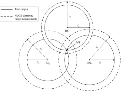
BS1 BS2 BS3 True ranges NLOS-corrupted range measurements MS ζ2 ζ3 ζ1 r3 r1 r2
Figure 2.4: The Range Measurements Suffer from the NOLS Errors.
radio signal is either reflected or diffracted by obstructions, and it must take extra time to arrive at the receiver. The additional propagation time is so-called the Non-Line-of-Sight (NLOS) error, and is always positive as presented in Fig. 2.4. The NLOS error is viewed as a killer issue for location estimation [27]. The excess part of the time measurements will result in range errors on the order of 513 meters and 436 meters in the mean and the standard deviation respectively [28], which inevitably makes a time-based location algorithm to fail.
2.3.2 Methods Proposed to Mitigate or Reduce the NLOS error
Identifying NLOS Error According to the Residual Analysis
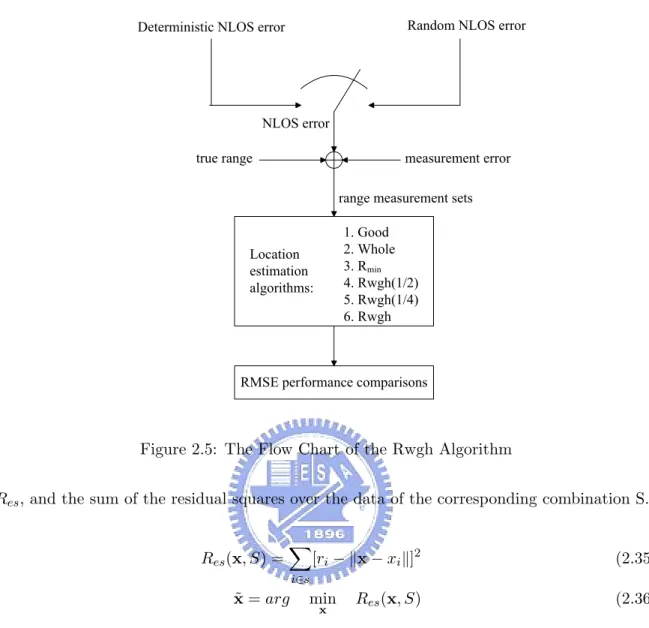
The residual weighting algorithm (Rwgh) proposed in [29] exploits the concept of the LS estimator and the weighting of each intermediate estimate to identify the NLOS error without any prior information. It takes three steps to figure out the NLOS error. First, it chooses a subset n from the N range measurements to form a range set where 2 < n ≤ N . Second, it proceeds the calculation of the intermediate LS estimate ˜x, which is the vector minimizes
Deterministic NLOS error Random NLOS error NLOS error measurement error true range Location estimation algorithms:
range measurement sets 1. Good 2. Whole 3. Rmin 4. Rwgh(1/2) 5. Rwgh(1/4) 6. Rwgh
RMSE performance comparisons
Figure 2.5: The Flow Chart of the Rwgh Algorithm
Res, and the sum of the residual squares over the data of the corresponding combination S.
Res(x, S) = X i∈s [ri− kx − xik]2 (2.35) ˜ x = arg min x Res(x, S) (2.36)
The estimated ˆRes containing NLOS measurement is deservedly larger than that of other estimates. Hence, the weighting is inversely proportional to ˆRes of the estimate. At last, the final estimates can be expressed as a weighted linear combination of the previous intermediate estimates.
The flow chart of this algorithm is shown in Fig. 2.5. Both Deterministic and random NLOS errors are concerned. The estimated ˆRes with varies numbers of range combinations
are compared with the all-LOS case and the case suffered from NLOS error. The performance shows that the Rwgh is effective to resist the NLOS error.
Identifying NLOS Error According to the Standard Deviations
The transmitted radio signal corrupted by the NLOS errors arrives at the receives through multiple channels. The characteristics of these channels can be obtained after acquiring enough statistical data. The standard deviation, a kind of prior information, is used in [30] to identify the NLOS error.
Once a radio signal reaches the receiver m, the range measurement rm(ti) is formulated by using an Nth order polynomial fit and its unknown coefficients is solved by the least
square techniques. A smoothed measurement sm(ti) utilizing the solved coefficients above is
presented as another Nth order polynomial function. The standard deviation at this moment
can be derived as ˆ σm = v u u t 1 K K−1X i=o (sm(ti) − rm(ti))2 (2.37)
Suppose that σm is the standard deviation of the LOS cases that is calculated when the
transmitter has LOS with the receiver m. It is well-known that the NLOS effect will increase the standard deviation of the range measurements in a great manner. According to the time history of range measurements, a decision hypothesis distinguishing NLOS from LOS is made as
H0 : ˆσm= σm (LOS case) (2.38)
H1 : ˆσm > σm (NLOS case) (2.39)
The NLOS-contaminated signal can be identified and corrected. The corrected signal can be proceeded with positioning and a better estimate is expected.
Identifying NLOS Error According to the Theoretic Decision Rules
The theoretic framework in [31] offers a binary hypothesis test to classify whether a range measurement is corrupted by NLOS error or not. It is assumed that the error distributions
can be categorized with respect to the NLOS and the LOS transmissions. The statistical characteristic of the LOS error is assigned as a Gaussian distribution with zero mean and variance σ2
los. The distribution of NLOS error is also modelled as Gaussian with mean µnlos
and variance σ2
nlos. It is noted that µnlos> 0 and σnlos2 > σ2los. The general binary hypothesis
test for NLOS identification is as followed.
H0 : X ∼ fXlos with prior probability P (H0) (LOS condition) (2.40) H1: X ∼ fXnlos with prior probability P (H1) (NLOS condition) (2.41)
Five cases are classified and summarized according to whether the probability model, prior probability, and the characteristic (i.e. the mean and variance) of NLOS error is known or not. Four different hypothesis tests are presented with different combinations of the above statistical information. It is worthy of mention that the fifth decision rule is the same with that of the previous approach when the model of NLOS distribution is unknown.
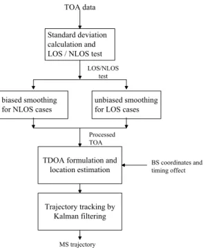
Mitigating NLOS Error by Using Kalman Filtering
The Kalman filter is commonly used in smoothing a data set or tracking an object. An application [32] applying two Kalman filters, one for smoothing and the other for tracking, proceeds the task of positioning in a NLOS environment. The method first periodically samples the received radio signals to gather enough data to estimate the standard deviation ˆ
σm, and identifies the NLOS-corrupted range measurements by the following hypothesis test.
H0: ˆσm= γσm (LOS case) (2.42)
H1: ˆσm> γσm (NLOS case) (2.43)
The σm is the standard deviation of the measurement noise in the LOS case. The presence of
γ is to reduce the false alarm probability. The classified LOS and NLOS range measurements in Fig. 2.6 are then passed to the Kalman filters behind. The smoothing procedure is taken to proceed the LOS range measurements to an unbiased Kalman filter, and the NLOS ones to
Standard deviation calculation and LOS / NLOS test
TOA data
unbiased smoothing for LOS cases biased smoothing
for NLOS cases
TDOA formulation and location estimation Trajectory tracking by Kalman filtering LOS/NLOS test Processed TOA BS coordinates and timing offect MS trajectory
Figure 2.6: Mobile location estimation using the Kalman Filtering
a biased Kalman filter. The NLOS error is mitigated step by step with the bias obtained at the sampling state. The proceeded TOA data are continuously fed to the process of location estimation. A Kalman filter finally handles these estimated position data of the mobile to acquire a smooth trajectory.
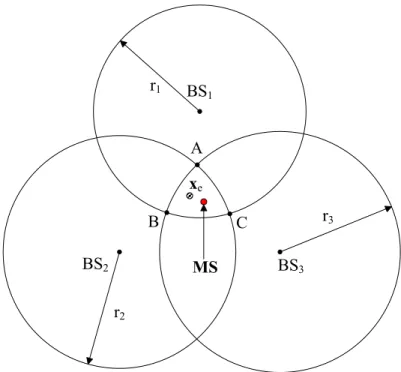
Mitigating NLOS Error According to the Properties of Geometry
The NLOS error is reduced in a cell-based layout without knowing the prior information of the range measurements [33]. In addition, a large number of base stations required in [29] are not necessary in this proposed method. A true range measurement is expressed as a multiplication of the corresponding measured range and a scale factor. The function of a scale factor is to scale a NOLS-corrupted range measurement to be closer to the true range. Each scale factor is varied from 0 to 1, and all the three scale factors form a vector v. The upper bound U of the vector v is [1 1 1]T. As shown in Fig. 2.7, a nonlinear equality g(v) is
derived by utilizing the law of cosines. The formula g(v) is a function of the measured ranges, the distance of any two of the three base stations, and the vector v.
BS1 BS2 BS3 A B C r3 r1 r2 MS θ1 θ2 θ3
Figure 2.7: The Geometry of the TOA-Based Location Showing the Relationship of the True Ranges and Inter-BS Distance.
In the Fig. 2.7, the limitations of the lower bound L of the vector v is characterized by confirming that any measured range circle must intersect with another two. The intersections A, B and C of the three measured ranges are the 3 closest points to the MS. A nonlinear cost function F (v) is then presented as the squared sum of the distances between the mobile station and these intersections. Given g(v) = 0 and the boundary of the vector v, the objective function F (v) is constraint-optimized with the applying of the sequential quadratic programming (SQP) algorithm to obtain the estimated scale vector ˆv as
ˆ
v = min
L≤v≤U F (v) subject to g(v) = 0 (2.44)
Finally, the MS location is decided by taking the estimated scale vector ˆv into any con-ventional location algorithms.
BS1 BS2 BS3 A B C r3 r1 r2 xe MS
Figure 2.8: Geometric Constraints for TOA-Based Location Estimation Confine the True MS’s Position in the Overlap Region of the Range Measurements.
Mitigating NLOS Error According to the Properties of Geometry and Noise Vari-ance
As illustrated in Fig. 2.8 , the MS’s location estimation using the Two-Step Least Square method may fall inside or outside of the boundaries of the three arcs, AB, BC, and CA. With the larger overlap region caused by the increasing NLOS error, the inaccuracy of the location estimation of the MS consequentially raises. The characteristics of the geometric layout and the noise variances are applied to a method named the Geometry-Constrained Location Estimation (GLE) algorithm [34] to modify the formulations within the Two-Step Least Square method. The primary objective of the proposed GLE algorithm is to confirm the location estimate within the overlap region by joining the geometric constraints into the Two-Step LS method.
the Two-Step Least Square method. The constrained cost function γ is given by γ = X µ=a,b,c 1 3kx − µk 2 1/2 (2.45)
where x is the MS’s location as mentioned before; a = (xa, ya), b = (xb, yb), and c = (xc, yc)
represent the corresponding coordinates of the points A, B, and C. The parameter γ defined as the square root of the average squared-sum of the distance from the MS to the three points A,B and C is called the virtual distance and obviously varies as the three coordinates a ,b and c changes. The corresponding expected virtual distance γe is defined as
γe = X µ=a,b,c 1 3kxe− µk 2 1/2 = γ + nγ (2.46)
where nγ is the error induced by the computed deviation between γe and γ. The xecalled the
expected MS’s position is chosen to minimize the deviation between the virtual distance γ and the corresponding expected virtual distance γe. The coordinates of the expected MS position xeis a linear combination of those of the three points A, B, and C with the parameters acting
as weights which is related to the signal variations.
xe= w1xa+ w2xb+ w3xc (2.47a) ye= w1ya+ w2yb+ w3yc (2.47b) where w` = σ 2 ` σ2 1 + σ22+ σ32 for ` = 1, 2, 3 (2.48)
σ1, σ2, and σ3 are the corresponding standard deviations obtained from the three TOA mea-surements r1, r2, and r3.
The selection of the weights is directly proportional to the corresponding signal variances. For example, the excessive range measurement r1 due to the comparatively large signal
vari-ance σ1 may probably cause the true position of the MS to move incorrectly toward to the boundary of the arc BC. Therefore,the weighting of the coordinates of a should be relatively large to make the true position of the MS to move toward the point A of the analogous triangle.
The GLE algorithm integrates the geometric constraints into the first step of the Two-Step Least Square method is defined as:
Hx = J + ψ (2.49) where x = · x y β ¸T H = −2x1 −2y1 1 −2x2 −2y2 1 −2x3 −2y3 1 −2γx −2γy 1 J = r2 1 − κ1 r2 2 − κ2 r2 3 − κ3 γ2 e− γκ
The corresponding coefficients are given by
β = x2+ y2 κ` = x2` + y`2 for ` = 1, 2, 3 γx = 1 3(xa+ xb+ xc) γy = 13(ya+ yb+ yc) γκ = 13(x2a+ x2b + x2c+ y2a+ y2b + yc2)
The noise matrix ψ in (2.49) can be obtained as ψ = 2 c Bn + c2n2 (2.50) where B = diag ½ ζ1, ζ2, ζ3, γ ¾ n = · n1 n2 n3 nγ/c ¸T
Based on the two-step LS scheme, an intermediate location estimate after the first step can be obtained as
ˆ
x = (HTΨ−1H)−1HTΨ−1J (2.51)
where
Ψ = E[ψψT] = 4 c2 BQB
It is noted that Ψ is obtained by neglecting the second term of (2.50). The matrix Q can be acquired as
Q = diag ½
σ12, σ22, σ23, σγ2e/c2 ¾
Q represents the covariance matrix for both the TOA measurements and the expected virtual distance, where σ2γe/c corresponds to the standard deviation of γe/c. The final location
esti-mation can be obtained by continuously carrying on the second step of the Two-Step Least Square method [22].
2.4
Studies on an Important Metric — Geometric Dilution of
Precision (GDOP)
The GDOP is a metric that describes the effect of different BS layouts on the performance of location algorithms. It is a measurement-to-noise ratio on standard deviation.
Let the distance ζi from the MS to the ith BS in 2-D condition is given as
ζi=
p
(x − xi)2+ (y − yi)2 i = 1, 2, ...N (2.52)
where (xi, yi) are the known coordinates of the ith BS, and (x, y) is the unknown position of
the MS. The matrix M is the partial deviations of the noise-free measurement equations with respect to the unknown parameters (i.e. x and y).
M = ∂ζ1 ∂x ∂ζ∂y1 ∂ζ2 ∂x ∂ζ∂y2 . . ∂ζN ∂x ∂ζ∂yN = x−x1 ζ1 y−y1 ζ1 x−x2 ζ2 y−y2 ζ2 . . x−xN ζN y−yN ζN (2.53)
The Best, Linear, Unbiased Estimate (BLUE) of (x, y) obtains the variance as
V ar(ˆx) = diag(MTQ−1M)−1 (2.54)
where the matrix Q is the noise covariance matrix. Define G2×2as
G = V ar(ˆx)
Q (2.55)
and the GDOP will be given by
GDOP =pG1,1+ G2,2 (2.56)
range measurements. If the noise errors are simplified by i.i.d. distribution with mean 0 and variance σ2
n, the matrix G will translate into
G = (MTM)−1 (2.57)
A statement in [35] demonstrates that given a Gaussian-distributed noise, the GDOP and the Cramer-Rao lower Bound (CRLB) are identical. In [36], the minimum GDOP inside a K-side (K ≥ 3) regular polygon takes place at the center of the layout and the value is √2
K. To verify
the conclusions in [36], a series of simulations with TOA or TDOA information are tried in a K-side regular polygon. The results show that the shape of the GDOP seems to be a concave function and the value at the center is minimum and comparable to √2
Chapter 3
The Location Estimation with The
Assistance of Virtual Base Stations
3.1
Overview
The Taylor-Series Estimation (TSE) algorithm [21] mentioned in section 2.1.5 transfers an original measurement range into a simplified form by a linearized process. The adoption of the first-order Taylor expansion for two variables notably simplifies the utilization of the Least Square (LS) method on the range data. The method takes the error covariance matrix into the formulation and views it as the weighting of the range data. An initial guess of the MS’s position is necessary for the algorithm to continue the estimation iteratively. A diverged result may occur due to a improper initial guess of the MS’s position. The two-step LS method in section 2.1.6 can use the TOA [22], the TDOA [23], or the hybrid TDOA/AOA [24] measurements to estimate the MS position. It is regarded as an implementation of a Maximum Likelihood (ML) estimator under the assumption of equal prior. After a linearized transformation of the independent-assumed objective parameters, a LS method is applied to estimate the MS position in the first step. The estimated result is fine tuned with the considerations of the presence of the estimation errors and the relationship of the objective parameters. The other LS process is carrying on to get the final estimate. Rather than
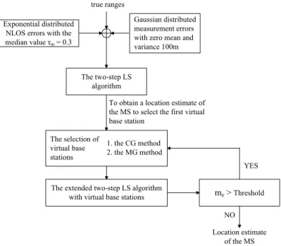
true ranges Exponential distributed
NLOS errors with the median value τm= 0.3 The two-step LS algorithm me> Threshold 1. the CG method 2. the MG method Location estimate of the MS YES NO To obtain a location estimate of the MS to select the first virtual base station The selection of virtual base stations Gaussian distributed measurement errors with zero mean and variance 100m
The extended two-step LS algorithm with virtual base stations
Figure 3.1: The Flow Chart of the VBS Algorithm
run iteratively, two-stepped process is enough in this algorithm. The LLOP algorithm [25] in section 2.1.7 uses the connections of the intersections of the measured range circles to estimate the MS position. There are CN
N −1 independent line equations generated by the intersections
of the N measured range circles. Two similar method, intersections of the line equations and the least squares, are applied to locate the MS position. However, the TSE, the two-step LS and the LLOP algorithms are only feasible for the LOS environments. The NLOS error be a killer issue in the location positioning will bring up a considerable bias in to a time measurement, especially in a dense region like metropolises and downtowns.
The method in [32] mitigates the influence of the NLOS error by utilizing the constraints of the geometric layout in the cell-based communication network. A constraint equation and a nonlinear cost function are derived from the characteristics of the geometry. The cost function is constraint-optimized by adopting the SQP algorithm. The computation time is intuitively increased duo to the optimization process. The Geometry-constrained Location Estimation (GLE) algorithm [34] extended from the two-step LS method is found effective and time-saving in location position. The proposed VBS (Virtual Base Stations) algorithm
takes a step ahead by combining the considerations of the signal variations with the extending geometric constraints of the virtual base stations. The functionalities of the assisted virtual base stations is to improve the GDOP effects by joining the geometric constraints into the formulations of the GLE algorithm. The flow chart of the proposed VBS algorithm is shown in Fig. 3.1. An exponential distributed NLOS error is considered. The first estimate ˆxM,1of the
MS’s position is obtained by utilizing the two-step LS method. The first assisted virtual base station xv,1 can then be obtained by applying the proposed Center-of-Gravity (CG) based or
the Minimum GDOP (MG) based selection methods. The second estimate ˆxM,2 of the MS’s
position obtained from the VBS algorithm is compared with the previous estimate ˆxM,1. The iteration processes will continue while the distance from the latest estimate to the last one is larger than the chosen threshold. The proposed VBS algorithm iteratively adds virtual base stations into the original layout and terminates as the estimated MS’s position converges.
3.2
Observations from the GDOP
The GDOP criterion is originally used in the satellite-based location system to check if the layout of the visible satellites is good for the goal of positioning. It has been applied to the cell-based location system as well. The interpretation of the meaning of the GDOP is that it represents the standard deviation ratio of the signal and the noise. In a fixed layout, the signal variations differ with where the MS locates. The radio signals range over larger variations not only raise the inaccuracy of the location estimation but also the value of the GDOP. In other words, the lower value of the GDOP stands for the smaller signal variations in a fixed layout and expectedly accompanies the better performance of location estimation. The GDOP is utilized as an index for judging the the effect of the geometric layout. Several K-side (3 ≤ K ≤ 6) regular polygon layouts are examined to verify the phenomenons of the GDOP. Each regular polygon is centered at the origin with the vertexes 1000m away from the origin. In each case, the 3-D graph and the contour of the GDOP value are shown in Fig. 3.2 to 3.5. Some results can be concluded inside the regular polygons by observing the differences of these figures.
−2000 0 2000 −2000 0 2000 0 0.5 1 1.5 2 2.5 3 x−axis The GDOP while using 3 TOA measurements
y−axis GDOP 1.2 1.3 1.4 1.5 1.6 1.7 1.8 1.9 −2000 0 2000 −3000 −2000 −1000 0 1000 2000 3000 x−axis y−axis GDOP(min)=1.1547 1.251 1.251 1.251 1.2029 1.2029 1.2029 1.2029 1.2029 1.2029 1.251 1.2992 1.3474 1.2029 1.2029 1.251 1.29921.3474 1.251 1.2992 1.4437 1.4918 1.6363 1.6845 1.829 1.251 1.2992 1.3955 1.4918 1.5882 1.7327 1.7327 1.2029 1.6845 1.3 1.4 1.5 1.6 1.7 1.8
Figure 3.2: The GDOP Value in a Regular Triangle.
−2000 0 2000 −2000 0 2000 0 0.5 1 1.5 2 2.5 3 x−axis The GDOP while using 4 TOA measurements
y−axis GDOP 1.05 1.1 1.15 1.2 1.25 1.3 −2000 0 2000 −3000 −2000 −1000 0 1000 2000 3000 x−axis y−axis GDOP(min)=1 1.0213 1.0213 1.0213 1.0213 1.0425 1.0425 1.0425 1.0425 1.0638 1.0638 1.0638 1.0638 1.0213 1.0213 1.0425 1.0425 1.0638 1.0638 1.0851 1.0851 1.0213 1.0213 1.1276 1.1489 1.2127 1.1489 1.2553 1.2766 1.2766 1.2553 1.05 1.1 1.15 1.2 1.25 1.3
−2000 0 2000 −2000 0 2000 0 0.5 1 1.5 2 2.5 3 x−axis The GDOP while using 5 TOA measurements
y−axis GDOP 0.9 0.95 1 1.05 1.1 1.15 1.2 1.25 1.3 −2000 0 2000 −3000 −2000 −1000 0 1000 2000 3000 x−axis y−axis GDOP(min)=0.89443 0.92168 0.92168 0.92168 0.92168 0.92168 0.92168 0.92168 0.92168 0.92168 0.92168 0.97617 0.97617 0.97617 0.97617 0.97617 1.0579 1.1669 1.0579 1.0307 1.0579 0.94893 0.94893 0.95 1 1.05 1.1 1.15 1.2 1.25 1.3
Figure 3.4: The GDOP Value in a Regular Pentagon.
−2000 0 2000 −2000 0 2000 0 0.5 1 1.5 2 2.5 3 x−axis The GDOP while using 6 TOA measurements
y−axis GDOP 0.85 0.9 0.95 1 1.05 1.1 1.15 −2000 0 2000 −3000 −2000 −1000 0 1000 2000 3000 x−axis y−axis GDOP(min)=0.8165 0.83883 0.83883 0.83883 0.83883 0.83883 0.83883 0.83883 0.83883 0.83883 0.83883 0.83883 0.83883 0.88349 0.88349 0.90583 0.97283 1.0398 0.99516 0.90583 0.95049 1.0622 0.92816 0.95049 0.99516 1.0622 0.95049 0.97283 1.0845 0.85 0.9 0.95 1 1.05 1.1 1.15
The shape of the GDOP is a concave function with the values at the vertexes being the maximum. The minimum GDOP is found to occur at the center and the value is comparably to √2
K in a K-side regular polygon. One thing to be noted is that the GDOP values are
smaller and the regions inside the regular polygons are flatter as K increases. According to the statements above, a virtual base station utilized in the VBS algorithm can be joined to the original layout to flatten the GDOP effect and lower the minimum value. The selection of a virtual base station is to let the estimated MS’s position locate at the location where the value of GDOP is minimum.
3.3
The Extended Two-Step LS Algorithm with Virtual Base
Stations
A series of geometric constraints involved by the assisted virtual base stations is feasible to be integrate into the GLE algorithm. The following section shows the way that how to integrate the information of the assisted virtual base stations into the conventional two-step LS algorithm.
3.3.1 Overview
Analogous to the GLE algorithm by adding geometric constraints within the conventional two-step LS method, the VBS algorithm extends the concept of ”virtual” assistances in the GLE algorithm to add the geometric constraints from the assisted virtual base stations.
As shown in Fig. 3.6, the three original range measurements intersects at the A, B and C points around the overlap region. A linear combination of the coordinates of the A, B and C points with the corresponding parameters direct proportional to the signal variances constructs the expected virtual distance as in (2.46). The expected virtual distance restricts the MS in the overlap region and constructs a cost function to minimize the deviation to the virtual distance as in (2.45). The functionality of the virtual base stations is to reduce the GDOP effect in the original layout. From the observations in section 3.2, the more the number
BS1 BS2 BS3 A B C r3 r1 r2 xe VB3 VB2 VB1
Figure 3.6: The Location Estimation with the Assistance of the Virtual Base Stations of the virtual base stations are, the lower the value of the GDOP is. With an appropriate setting of the threshold, the precision of the location can be achieved.
3.3.2 Formulation of the Extended Two-Step LS Algorithm
While the concept of the ”virtual” assistance in the proposed VBS algorithm is the same with that of the GLE algorithm, the formulations of the expected virtual distance γe as
in (2.46) and the definition of the weights as in (2.48) are utilized. In order to integrate the information of the ith added virtual base station with the geometric constraints, the coordinates of the ith virtual base station (xv,i, yv,i) is expressed as
xv,i = αa,ixa+ αb,ixb+ αc,ixc for i = 1, 2, ... , n (3.1)
yv,i = αa,iya+ αb,iyb+ αc,iyc for i = 1, 2, ... , n (3.2)
are acquired. The parameters αa,i, αb,i and αc,i can be obtained by solving (3.1) and (3.2) associated with αa,i+ αb,i+ αc,i= 1. The fraction 13 in (2.46) is substituted by the parameters
αa,i, αb,i and αc,i so that the expression of the γe,i can be formulated as
γe,i= X µ=a,b,c αµ,ikxe− µk2 1/2 = γ + nγi (3.3)
where nγ,i is the error of between the γ and the γe,i.
It is assumed that there are n virtual base stations collaborating in the VBS algorithm. By rearranging and combining (2.1) and (2.46) in the matrix format, the following equation can be obtained: Hx = J + ψ (3.4) where x = · x y β ¸T H = −2x1 − 2y1 1 −2x2 − 2y2 1 −2x3 − 2y3 1 −2xv,1 − 2yv,1 1 −2xv,2 − 2yv,2 1 . . . −2xv,n − 2yv,n 1
J = r2 1 − κ1 r2 2 − κ2 r2 3 − κ3 γe,1− γκv,1 γe,2− γκv,2 . . γe,3− γκv,n
The corresponding coefficients are given by
β = x2+ y2 (3.5)
κ` = x2` + y`2 for ` = 1, 2, 3 (3.6) γκv,i = αa,i(x2a+ y2a) + αb,i(x2b + yb2) + αc,i(x2c+ y2c) (3.7)
It is noted that the equation (3.7) is utilized to facilitate the formulation of the two-step LS problem. Moreover, the noise matrix ψ in (3.4) can be obtained as
ψ = 2 c Bn + c2n2 (3.8) where B = diag ½ ζ1 ζ2 ζ3 γ1 γ2 ... γn ¾ (n+3)×(n+3) n = · n1 n2 n3 nγ1/c nγ2/c ... nγn/c ¸T (n+3)×1
Based on the two-step LS scheme, an intermediate location estimate after the first step can be obtained as
ˆ
where
Ψ = E[ψψT] = 4 c2 BQB
It is noted that Ψ is obtained by neglecting the second term of (3.8). The matrix Q can be acquired as Q = diag ½ σ2 1 σ22 σ32 σ2γe,1/c σ 2 γe,2/c ... σ 2 γe,n/c ¾
It can be observed that Q represents the covariance matrix for both the TOA measurements and the expected virtual distance, where σ
|γe,i|
1
2 corresponds to the standard deviation of
|γe,i|
1
2. The final location estimation after the second step of the two-step LS algorithm can
be obtained by referring the approach as stated in [23].
3.4
The Selection of a Virtual Base Station
Since the information of the virtual base stations can be integrated into the conventional two-step LS method, two methods of selecting virtual base stations are proposed hereafter.
3.4.1 The Center of Gravity (CG) Based Selection Method
As discussed in the section 3.2, the value of the GDOP at the center of the gravity is minimum in a regular polygon. A virtual base station is added to make the latest location estimate of the MS be at the center of the gravity of the modified layout. After the first location estimate ˆxM,1of the MS by the two-step LS method in a regular triangle layout, the
first virtual base station ˆxv,1 is added in accordance with the CG based selection method by
ˆ
xM,1= x1+ x2+ x3+ xv,1
BSN + V BN (3.10)
where the BSN and the VBN are the number of the base stations and the virtual base stations, respectively. The BSN and the VBN are 3 and 1 in this case. The first added virtual base station xv,1 can be obtained as 4ˆxM,1− 3xCG after a simple transformation while xCG is the position of the center of the gravity in the original layout. The first obtained virtual base