一個針對可調視訊編碼中跨層編碼與位元流擷取之位元率-失真最佳化模型

全文

(1)一個針對可調視訊編碼中跨層編碼與位元流擷取之位元率-失真最佳化模型. A Rate-Distortion Optimization Model for SVC Inter-layer Encoding and Bitstream Extraction 研究生：黃雪婷. Student：Hsueh-Ting Huang. 指導教授：彭文孝. Advisor：Wen- Hsiao Peng. 國立交通大學多媒體工程研究所碩士論文. A Thesis Submitted to Institute of Multimedia Engineering College of Computer Science National Chiao Tung University in partial Fulfillment of the Requirements for the Degree of Master in. Computer Science July 2008 Hsinchu, Taiwan, Republic of China. 中華民國九十七年七月.

(2) 一個針對可調視訊編碼中跨層編碼與位元流擷取之位元率-失真最佳化模型研究生：黃雪婷. 指導教授：彭文孝. 國立交通大學多媒體工程研究所. 摘. 碩士班. 要. 可調視訊編碼標準(SVC)使觀看裝置可以使用位元流擷取機制調整其視訊接收內容。正因可調視訊編碼提供了結合空間、時間與畫質上的可調性，為不同觀看裝置擷取適當的位元流時需要經過特別考慮，不適當的選擇經常會產生粗劣的觀賞品質。在本論文中，我們提出了一個針對可調視訊編碼位元流進行位元率-失真 (R-D)最佳化擷取的方法。精確地說，我們針對可調視訊編碼壓縮時的量化參數與跨層編碼相依性之設定，發展一組可適應性規則，遵循此規則所產生的良適性可調視訊編碼位元流(Well-adapted SVC bitstream)可在連續增益步驟中所擷取之可調層產生明顯較好的位元率-失真平衡。我們亦正式定義最佳化與近似最佳化擷取路徑的概念，並設計了在運算量上相當有效率的擷取路徑搜尋策略。實驗的結果展示出我們的位元率-失真最佳化的適應性設定方法與擷取策略可在不同觀賞裝置的播放畫面品質達到重大的改善。特別的是，我們的可適應性規則可保證沿著所找出的最佳擷取路徑之位元率-失真曲線具有凸狀的特性，並使得貪婪探索式擷取策略(Greedy Heuristic)可用以找出最佳化或近似最佳化之路徑，而此最簡單之搜尋策略比起暴力搜尋法(Exhaustive Search)只需要大約一半的運算複雜度。.

(3) A Rate-Distortion Optimization Model for SVC Inter-layer Encoding and Bitstream Extraction Student：Hsueh-Ting Huang. Advisors：Wen-Hsiao Peng. Institute of Multimedia Engineering National Chiao Tung University. ABSTRACT The Scalable Video Coding (SVC) standard enables viewing devices to adapt their video reception using bitstream extraction. Since SVC offers spatial, temporal, and quality combined scalability, extracting proper bitstreams for different viewing devices can be a non-trivial task, and naive choices usually produce poor playback quality. In this thesis, we propose an approach for performing rate-distortion (R-D) optimal extraction of SVC bitstreams. Specifically, we developed a set of adaptation rules for setting the quantization parameters and the inter-layer dependencies among the SVC encoding layers. A well-adapted SVC bitstream thus produced manifest good R-D trade-offs when its scalable layers are extracted in successive refinement steps. We also formalized the notion of optimal and near-optimal extraction paths and devised computationally efficient strategies to search for the extraction paths. Experimental results demonstrated that our R-D optimized adaptation schemes and extraction strategies offer significant improvement in playback picture quality on various viewing devices. In particular, our adaptation rules promise R-D convexity along optimal extraction paths and permit the greedy heuristic extraction strategy to be used for discovering the optimal/near-optimal paths. This simplest strategy performs only half of the computation necessary for an exhaustive search..

(4) 誌. 謝. 首先我要感謝彭文孝老師與邵家健老師一直以來給予我研究上的指導，經由一次次與老師的討論，研究內容才得以逐漸趨於完整；若沒有兩位老師所給予的方向指引與協助，我將無法完成這項工作。這兩年來，老師對於研究的熱情與嚴謹態度、解決問題的思考方式，一直是我學習的典範；老師的指導與建言，經常使我獲益良多。對於老師平時給我的鼓勵與支持，這份感激之情更是筆墨難以形容。其次，我要感謝王澤瑋學弟幫忙跑了很多的實驗與整理數據；感謝林哲民同學參與討論中提出的意見；感謝林岳進同學提供實驗中的時間差補法程式；感謝李志鴻學長、林鴻志學長、陳漪紋學長在我有疑問時為我解答；感謝所有 MAPL 實驗室裡的成員，包含：林岳進、陳敏正、Eric、陳俊吉、陳建穎、林哲永、詹家欣、王澤瑋、吳思賢，無論是研究上的討論或生活中的苦樂分享，你們是我研究生涯不可或缺的伙伴。最後也最重要的，我要感謝長久以來給我關心與鼓勵、支援我完成碩士班學業的父母：黃慶峯先生與黃吳素真女士，若沒有您們的支持就不會有今日的我；也要感謝我的姐妹黃慧玲與黃綉雯、以及 Puppy，感謝你們一路的陪伴打氣給了我很多力量，謝謝你們！.

(5) A Rate-Distortion Optimization Model for SVC Inter-layer Encoding and Bitstream Extraction Advisors: Prof. Wen-Hsiao Peng Prof. John Kar-Kin Zao Student: Hsueh-Ting Huang Institute of Multimedia Engineering National Chiao-Tung Univeristy 1001 Ta-Hsueh Rd., 30010 HsinChu, Taiwan July 2008.

(6) Contents. Contents. i. List of Tables. iv. List of Figures. v. 1 Research Overview. 1. 1.1 Introduction . . . . . . . . . . . . . . . . . . . . . . . . . . . . . . . . .. 1. 1.2 Problem Statement . . . . . . . . . . . . . . . . . . . . . . . . . . . . .. 2. 1.3 Contributions and Organization of Thesis . . . . . . . . . . . . . . . . .. 2. 2 Background. 4. 2.1 Scalable Video Coding . . . . . . . . . . . . . . . . . . . . . . . . . . .. 4. 2.1.1. Concept . . . . . . . . . . . . . . . . . . . . . . . . . . . . . . .. 4. 2.1.2. Transport Interface of SVC . . . . . . . . . . . . . . . . . . . .. 5. 2.2 Related Works . . . . . . . . . . . . . . . . . . . . . . . . . . . . . . . .. 7. 2.2.1. Basic Extraction . . . . . . . . . . . . . . . . . . . . . . . . . .. 7. 2.2.2. Quality Information Table (QIT) . . . . . . . . . . . . . . . . .. 7. 2.2.3. Quality Index (QI) . . . . . . . . . . . . . . . . . . . . . . . . .. 8. 2.2.4. Quality Layer Optimized Extraction . . . . . . . . . . . . . . .. 9. -i-.

(7) CONTENTS 3 Rate-Distortion Optimization of SVC Bitstream Extraction 3.1 Extraction Paths through SVC Bitstream. 11. . . . . . . . . . . . . . . . .. 11. 3.1.1. Successive Refinement . . . . . . . . . . . . . . . . . . . . . . .. 12. 3.1.2. Incremental and Cumulative Rate-Distortion Performance . . .. 12. 3.2 Rate-Distortion Optimal Extraction Path . . . . . . . . . . . . . . . . .. 14. 3.3 Near-optimal Extraction Paths . . . . . . . . . . . . . . . . . . . . . .. 14. 4 Searching for Optimal Extraction Paths 4.1 Graphical Tools. 16. . . . . . . . . . . . . . . . . . . . . . . . . . . . . . .. 16. 4.2 Search Strategy . . . . . . . . . . . . . . . . . . . . . . . . . . . . . . .. 19. 4.2.1. Dynamic Programming Algorithm . . . . . . . . . . . . . . . . .. 19. 4.2.2. Greedy Heuristic Scheme . . . . . . . . . . . . . . . . . . . . . .. 21. 4.3 Analysis of Greedy Heuristic Scheme . . . . . . . . . . . . . . . . . . .. 23. 4.3.1. Convex Segments and Global Condition . . . . . . . . . . . . .. 23. 4.3.2. Strong Local Conditions . . . . . . . . . . . . . . . . . . . . . .. 24. 4.3.3. Weak Local Conditions . . . . . . . . . . . . . . . . . . . . . . .. 25. 4.3.4. Fractional Violation of Local Conditions . . . . . . . . . . . . .. 26. 4.4 Summary . . . . . . . . . . . . . . . . . . . . . . . . . . . . . . . . . .. 27. 5 Production of Well-adapted SVC Bitstreams. 28. 5.1 Settings of Quantization Parameters . . . . . . . . . . . . . . . . . . .. 28. 5.2 Settings of Inter-layer Dependencies . . . . . . . . . . . . . . . . . . . .. 29. 6 Experiments. 32. 6.1 Implementation of Well-adapted SVC Bitstream . . . . . . . . . . . . .. 32. 6.1.1. Prediction of R-D Convexity . . . . . . . . . . . . . . . . . . . .. 32. 6.1.2. Degradation in Coding Efficiency . . . . . . . . . . . . . . . . .. 34. 6.2 Analysis of Optimal Extraction Paths . . . . . . . . . . . . . . . . . . .. 35. 6.2.1. Optimal Paths versus Video Contents . . . . . . . . . . . . . . .. 36. 6.2.2. Optimal Paths versus Distortion Measures . . . . . . . . . . . .. 36. 6.2.3. Optimal Paths versus Spatiotemporal Interpolation . . . . . . .. 38. 6.3 Performance of Greedy Heuristic Scheme . . . . . . . . . . . . . . . . .. 39. 6.3.1. Extraction Paths and R-D Performance . . . . . . . . . . . . . .. 39. 6.3.2. Computational Complexity . . . . . . . . . . . . . . . . . . . . .. 40. -ii-.

(8) CONTENTS 6.4 Comparisons with Other Extraction Schemes . . . . . . . . . . . . . . .. 41. 7 Conclusions. 45. Bibliography. 47. -iii-.

(9) List of Tables. 6.1 Testing conditions and encoder parameters . . . . . . . . . . . . . . . .. 36. 6.2 Comparison of extraction paths with MSE. . . . . . . . . . . . . . . . .. 41. -iv-.

(10) List of Figures. 2.1 SVC dependency structure . . . . . . . . . . . . . . . . . . . . . . . . .. 5. 2.2 Scalable layers corresponding to Figure 2.1 . . . . . . . . . . . . . . . .. 6. 2.3 Preference path of perceptual quality [4] . . . . . . . . . . . . . . . . .. 8. 2.4 Quality-Layer-based extraction [2] . . . . . . . . . . . . . . . . . . . . .. 9. 3.1 Measuring components of the deviation from convexity of a NAL cluster along an SVC R-D curve . . . . . . . . . . . . . . . . . . . . . . . . . .. 15. 4.1 R-D mesh and trellis diagram of an SVC test bitstream, Akiyo (CIF30). 18. 4.2 Example: using dynamic programming algorithm to find the optimal extraction path. . . . . . . . . . . . . . . . . . . . . . . . . . . . . . . .. 20. 4.3 Example: using greedy heuristic scheme to find the optimal extraction path. . . . . . . . . . . . . . . . . . . . . . . . . . . . . . . . . . . . . .. 22. 4.4 A trellis diagram with convex segments satisfying strong intra-trellis (local) and inter-trellis (global) R-D conditions . . . . . . . . . . . . . .. 25. 4.5 A trellis diagram with convex segments satisfying weak intra-trellis (local) and inter-trellis (global) R-D conditions . . . . . . . . . . . . . . .. 26. 4.6 R-D mesh and trellis diagram of an SVC bitstream with fractional violation of intra-trellis (local) R-D conditions . . . . . . . . . . . . . . . . -v-. 27.

(11) LIST OF FIGURES 5.1 R-D performance of SVC bitstreams with different inter-layer dependency settings. Labels A, B, C, D, and E denote five coding layers of different SNR levels with E being the target layer for reconstruction. . .. 30. 6.1 Comparison of SVC dependency settings: (a) Mobile and (b) Foreman. The results were produced with bottom-up encoding process and fixedquality configurations. . . . . . . . . . . . . . . . . . . . . . . . . . . .. 33. 6.2 Comparison of SVC dependency settings: (a) Mobile and (b) Foreman. The results were produced with bottom-up encoding process and fixedrate configurations. . . . . . . . . . . . . . . . . . . . . . . . . . . . . .. 34. 6.3 Comparison of total bit rate for different dependence settings. Fixedquality (FQ) and fixed-rate (FR) configurations were used. . . . . . . .. 35. 6.4 Comparison of optimal extraction paths for different viewing devices: (a) Mobile, (b) Foreman, (c) Akiyo, and (d) ICE. B.Direct and MSE are used for temporal interpolation and distortion measure, respectively. . .. 37. 6.5 Comparison of optimal extraction paths found by using MSE and MOS as the distortion criterion: (a) Foreman CIF@30 and (b) Mobile CIF@30. 38 6.6 Comparison of optimal extraction paths using frame replication (F.R.) and B_Direct_16x16 (B.Direct) for temporal interpolation: (a) Akiyo CIF@30 and (b) Foreman QCIF@30. . . . . . . . . . . . . . . . . . . .. 39. 6.7 Comparison of extraction paths for the steepest-descent method and exhaustive search: (a) R-D trellis diagram and (b) R-D curves. . . . . .. 41. 6.8 R-D preformance comparison of the proposed scheme with the Quality Layer and Basic extractions in JSVM 9: (a) QCIF SNR Scalability, (b) QCIF/CIF Combined Scalability. . . . . . . . . . . . . . . . . . . . . .. 42. 6.9 Bitstream extraction (a) with and (b) without successive refinement. R1-R4 indicate the extracted NAL sets associated with increasing bit rate. 43. -vi-.

(12) CHAPTER 1. Research Overview. 1.1. Introduction. Production of scalable bitstreams that can be played back by a garden variety of viewing devices has been a long pursued goal of video compression technology. The new scalable extension of H.264/AVC standard (referred hereafter as SVC) [12][16] promises to achieve that goal by employing adaptive inter-layer prediction along with hierarchical temporal reference. By encoding a video sequence into an inter-dependent set of network abstraction layer (NAL) units, SVC allows different viewing devices to extract and decode different scalable layers according to their display formats, processing power, and/or transport network throughput. However, the parts of a bitstream needed for providing good quality playback at different devices may differ significantly depending on the visual characteristics of video programs, the quantization and dependency settings of SVC encoders as well as the display formats of viewing devices. This problem has prompted an intensified study of bitstream adaptation for viewing quality optimization.. -1-.

(13) Chapter 1. Research Overview. 1.2. Problem Statement. While offering the flexibility for discretionary bitstream extraction, the current standard does not specify what to produce and what to use if there are several extraction possibilities. Several approaches have thus been proposed for finding optimal bitstream adaptation/extraction schemes that ensure the best playback quality on a viewing device while making the best use of available transport bandwidth. Although the extraction process can be improved by R-D optimization, the playback quality may still be far from satisfactory. This is because the pre-encoded SVC bitstreams may not be well-adapted, which could easily give rise to poor R-D performance. As a result, in this thesis we propose a novel R-D optimization model to tackle the problem from both encoder settings and extraction process. Experiments were conducted to illustrate 1. How the tuning of quantization parameters coupled with the changing of interlayer dependencies affects the R-D performance of SVC bitstreams, 2. What criteria on SVC encoder/decoder settings may ensure the existence of optimal or near-optimal extraction paths for different viewing devices, 3. And how the optimal extraction paths of different viewing devices can be found using computationally efficient strategies especially when the SVC bitstream is to be extracted through successive refinements. Aiming at viewing quality optimization for bitstream adaptation of different devices, this thesis provides an in-depth study on the relationship among video contents, viewing device capability and searching strategies for finding an optimal extraction path. Moreover, SVC inter-layer dependency and quantization parameter settings during SVC encoding were investigated to discover some rules to produce well-adapted SVC bitstream.. 1.3. Contributions and Organization of Thesis. Specifically, our main contributions in this work include the following: • We define the rate-distortion optimal bitstream extraction problem as a constrained optimization problem and create a R-D trellis diagram to model the bitstream extraction process. • We employ dynamic programming algorithm and propose a fast greedy heuristic -2-.

(14) Chapter 1. Research Overview search strategy for searching optimal extraction paths. • We develop a set of adaptation rules for setting quantization parameters and inter-layer dependencies during SVC encoding. • We analyze a lot of experimental results to figure out how video contents, device types, distortion measures and interpolation algorithms may affect the optimal extraction paths. Experimental results indicate that our optimization scheme makes a significant difference in improving viewing quality. Our adaptation rules promise the R-D convexity of optimal extraction paths and enable the greedy heuristic scheme to achieve the same or similar performance as the dynamic programming algorithm while reducing the complexity by 50% or more. The remaining of this thesis is organized as follows: Chapter 2 contains a review of SVC dependency structure and related works for finding optimal bitstream extraction schemes. Chapter 3 presents our R-D optimization model for bitstream extraction. Chapter 4 introduces and analyses our strategies for finding an optimal/near-optimal extraction path. Chapter 5 further describes the necessary criteria that must be satisfied during SVC encoding in order to guarantee the existence of optimal/near-optimal extraction paths. Chapter 6 addresses the implementation issues of establishing welladapted inter-layer dependencies and provides a detailed analysis on the optimal extraction paths and evaluates the performance of the greedy heuristic scheme in search for the optimal path. The differences between our extraction scheme and other previous works are also compared. This thesis ends with a summary of our observations and a list of future works in the conclusion.. -3-.

(15) CHAPTER 2. Background. 2.1 2.1.1. Scalable Video Coding Concept. The scalable video coding (SVC) standard [3][12][16] is an scalable extension of the H.264/AVC standard developed by the Joint Video Team (JVT) that makes a single bitstream to provide multiple frame sizes, frame rates and quality levels while achieving a reasonable coding efficiency. A subset of SVC bitstreams can be extracted and decoded to produce a lower playback quality rather than failed to decode under some constraints of resources such as network throughput or power of devices. SVC supports three types of scalabilities: spatial, temporal and quality scalabilities. An SVC bitstream is organized into one base layer and one or more enhancement layers in corresponding dimension if it provides certain scalability. The spatial scalability bases on multilayer coding that uses separate encoder loops for different spatial resolution layers and develops adaptive inter-layer prediction techniques to exploit correlations among the layers. For each coding layer, the temporal scalability is provided by hierarchical temporal prediction structures. Quality scalability in SVC is provided -4-.

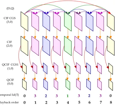
(16) Chapter 2. Background. (D,Q) CIF CGS (3,0). CIF (2,0). QCIF CGS1 (1,0). QCIF (0,0). Temporal Id(T). 0. 3. 2. 3. 1. 3. 2. 3. 0. Playback order. 0. 1. 2. 3. 4. 5. 6. 7. 8. Figure 2.1: SVC dependency structure. by two approaches: Coarse-grain quality scalable coding (CGS), which can be considered as a special case of spatial scalability with identical frame sizes for base and enhancement layer, and medium-grain quality scalable coding (MGS), which provides quality refinement layers inside each spatial layer and allows packet-based quality scalable coding. Figure 2.1 depicts an example of SVC dependency structure. Each block denotes a coded picture. The horizontal order presents playback order of frames and the vertical stack appears the coding layers, as known as dependency layers, in spatial/CGS scalabilities. The arrows present the dependency relations due to coding prediction structures. Every dependency layer may choose one of lower layers as reference layer for inter-layer prediction. To decode correctly, all of lower layers which target layer directly or indirectly depends on for reference should appear while bitstream decoding.. 2.1.2. Transport Interface of SVC. The coded video data and other side information in SVC bitstreams are encapsulated as network abstraction layer (NAL) units. The NAL unit consists of a header followed by payload data. The SVC NAL header consists of one-byte H.264/AVC header and three-byte extended SVC header. The extended header includes syntax elements de-5-.

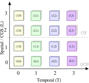
(17) Chapter 2. Background. Spatial / CGS (L). 3. (3,1,0) (3,0). (3,1,1) (3,1). (3 ,1,2) (3,2). (3,1,3) (3,3). (3,1,0) (2,0). (3,1,1) (2,1). (3,1,2) (2,2). (3,1,3) (2,3). 1. (1,1,0) (1,0). (1,1,1) (1,1). (1,1,2) (1,2). (1,1,3) (1,3). 0. (0,1,0) (0,0). (0,1,1) (0,1). (0,1,2) (0,2). (0,1,3) (0,3). 1. 2. 2. 0. CIF. QCIF. 3. Temporal (T). Figure 2.2: Scalable layers corresponding to Figure 2.1. pendency_id (D), temporal_id (T ) and quality_id (Q), which denote the identifier of dependency layers, temporal layers and quality refinement layers respectively, as well as other assisting information to support easy bitstream extraction. Another important syntax element is the priority identifier priority_id, which can be used to signal the importance of NAL unit. The sets of NAL units with identical D, T and Q information are organized into scalable layers. Here, the dependency and quality identifiers are combined as coding layer identifier L. As shown in Figure 2.2, the NAL units in the SVC bitstream which is depicted in Figure 2.1 can be grouped into scalable layers using coding layer identifier L and temporal identifier T . A set of scalable layers which are required for decoding certain corresponding scalable layer is known as scalable layer representation and defined as S(L, T ) in this thesis. For instance, S(3, 2) includes all scalable layers with identifiers L ≤ 3 and T ≤ 2 in Figure 2.2. SVC also designs Scalability information Supplemental Enhancement Information (SSEI) messages to carry the scalable layers information of bitstream such as spatial resolution, bit rate and priority information of layers for assisting bitstream adaptation processes.. -6-.

(18) Chapter 2. Background. 2.2. Related Works. 2.2.1. Basic Extraction. Currently, the Joint Scalable Video Model (JSVM) [11][15] provides three different ways to perform bitstream extraction. The first one is to extract a substream according to a bit rate constraint. The scalable layer representation thus extracted will have a bit rate that is closest to but not greater than the target bit rate. The second one is to choose a target scalable layer. The extractor will return the layer representations on which the target layer directly or indirectly depends. The last one is to explicitly specify the desired frame rate, frame size, and bit rate. However, the current standard does not specify what to produce if there are several extraction possibilities. In following subsection, we reviewed some approaches that have been proposed for finding optimal bitstream extraction schemes.. 2.2.2. Quality Information Table (QIT). Kim et al. [4] evaluated the perceptual preference for spatial and temporal quality over a range of bit rates to find preference paths of perceptual quality for bitstream extraction. The spatiotemporal switching points were recorded using Quality Information Tables (QIT), which were further provided to the extractor. The main idea is to figure out the optimal bit rate allocation strategy for three scalabilities of SVC according to video classes. First of all, video segments are classified and represented using semantic concepts. Then, quality preference paths between multidimensional scalabilities of different semantic concepts are determined by subjective testing while bit rate decreasing. For example, Figure 2.3[4] shows the preference paths of scenery and active concepts in three-dimensional scalability. The quality preference path of each video class is recorded in quality information table, which contains scalable layers information and relative bit rate of every switching point. After all, the QITs are provided to extractor for bitstream adaptation. This approach can find quality preference paths of perceptual quality for different video classes. However, the display formats of target devices are not considered. Furthermore, subjective testing is time consuming and hardly performed for all video sequences. -7-.

(19) Chapter 2. Background. Figure 2.3: Preference path of perceptual quality [4] : (a) scenery concept, (b) action concept. 2.2.3. Quality Index (QI). Unlike QIT used subjective testing as measurement, Lim et al.[7] defined a objective Quality Index (QI) to measure the perceptual quality and performed bitstream extraction by maximizing the quality index of the resulting bitstream subject to the bit rate constraint. The total QI is composed of weighted quality indexes of spatial, temporal and quality scalabilities (denote as QISR , QIF R and QIP SNR , respectively) of extracted bitstream. Among them, quality indexes for spatial scalability QISR and quality scalability QIP SNR can be measured by PSNR value. While measuring QISR , video segments are interpolated first to matching the playback format of target devices. Quality index for temporal scalability QIF R , on the other hand, employs an expo-logarithm function [5] as model to estimate subjective perceptual quality MOS. This scheme measures QI of every scalable layer representations that can be extracted subject to the bit rate constraint and chooses the one that has maximum total QI value. It obtains the sub-stream with best viewing quality measured by QI given any bit rate. But, the arbitrary extracted scalable layers at different bit rates may not support multiple adaptation of single extracted bitstream, which is an important feature in some network applications such as video multicasting.. -8-.

(20) Chapter 2. Background. Figure 2.4: Quality-Layer-based extraction [2]. 2.2.4. Quality Layer Optimized Extraction. Amonou et al. [2] formulated the problem as a rate-distortion (R-D) optimization process and shuffled the quality increments in an R-D sense for MGS/FGS enhancement layers. The idea is similar to Quality Layers in JPEG 2000 [14]. Priorities are assigned to NAL units in SVC bitstream to represent virtual layered organization of stream for further bitstream adaptation. First of all, R-D information is calculated for quality increment of each picture at each quality refinement level using independent or dependent distortion calculation. In dependent distortion calculation, the distortion of a picture and the distortion of pictures which were predicted from it are all considered. Namely, the impact on total rate and on the global reconstruction quality of each quality increment is computed to measure its R-D performance (slope). Based on the R-D information, the quality increments are sorted while the constraints of temporal prediction dependency are respected. Finally, Quality Layers are assigned to the quality increments according to the sorting results and stored in NAL header using priority_id field or in SEI messages. The Quality Layer optimized extraction can even apply to multiresolution bitstream. Figure 2.4 [2] illustrates Quality-Layer-based extraction. Each big block represents a scalable layer refereed to as (Dd , Tt , Qq ) where Dd indicates the spatial resolution, Tt for temporal layer and Qq for the quality level. The small blocks represent the NAL units of quality enhancement layer in different spatial resolution: dark-gray -9-.

(21) Chapter 2. Background blocks for D0 and gray ones for D1 . The blocks are ordered according to their Quality Layer information rather than quality levels. Therefore, NAL units with lower R-D performance will be dropped first when bitstream extraction happened. Quality Layer assignment makes quality increments are well prioritized, which insures a simple parsing of the stream that can be performed in network transmission. Nevertheless, the trade-off between spatial and temporal scalabilities is not considered in this approach. In summary, all of prior studies were designed to determine the bitstream extraction order through different optimization schemes except the Basic Extraction approach. Between them, the Quality-Layers-based extraction is the only one approach that can produce extracted sub-streams which can support multiple adaptations. Moreover, they all can be treated as post-processing of pre-encoded bitstreams. No suggestions for proper parameter settings during SVC encoding have been proposed for benefiting the bitstream extraction.. -10-.

(22) CHAPTER 3. Rate-Distortion Optimization of SVC Bitstream Extraction. Our investigation began with an attempt to devise strategies for finding an optimal extraction path of an SVC bitstream for a viewing device. The extraction path should be amenable to successive refinement of the SVC bitstream for supporting multiple adaptations. In this chapter, we describe the notion of successive refinement of optimal extraction paths and define the R-D optimization of SVC bitstream extraction problem as a constrained optimization problem. We further introduce a R-D trellis diagram to model the bitstream extraction process. Based on R-D trellis diagrams, we can employ dynamic programming algorithm to find the solution, and furthermore propose a greedy heuristic scheme to achieve the same or similar performance while reducing the complexity significantly.. 3.1. Extraction Paths through SVC Bitstream. While playing back an SVC bitstream, a viewing device may choose to extract and decode various sets of scalable layers (with possible use of error concealment) based -11-.

(23) Chapter 3. Rate-Distortion Optimization of SVC Bitstream Extraction on its display format, decoding capability and network throughput. A sequence of these scalable layer sets arranged from lowest scalable layer (referred to as base unit, ˆ Tˆ)) according to S(L, T )) to the target scalable layer (referred to as target layer, S(L, their dependence relations is known as an extraction path Π℘ for the viewing device. The subscript ℘ indicates a denotation of the extraction path.. 3.1.1. Successive Refinement. Beside of satisfying the dependence relations, one may want to fulfill some additional criteria while choosing the extraction paths for one or more viewing devices: 1. One may want to feed a viewing device with scalable layer representations of lower bit rates when the network throughput deteriorates. Such an act of bit-rate adaptation enables a viewing device to support graceful degradation of playback quality. 2. One may want to perform successive extraction en-route a multicasting tree. Significant reduction of transport bandwidth can be achieved by having an up-stream provider extracts only the scalable layers needed by its down-stream subscribers. Careful selection of extraction paths for different down-stream subscribers may minimize the bandwidth consumption of a multicasting session [9]. The two criteria of successive refinement of SVC bitstream imply that every element along the extraction path must have the previous element being its proper subset [Figure 6.9 (a)] for supporting multiple adaptations.. 3.1.2. Incremental and Cumulative Rate-Distortion Performance. Several extraction paths are available for traversing an SVC bitstream between the base unit and a target layer. These extraction paths are differentiated by their rate-distortion (R-D) performance, which measures the effectiveness that an extracted bitstream uses their data bits to enhance the quality of their playback pictures. The R-D performance of an SVC bitstream can be quantified in two ways using: (1) a ratio between the increase in bit rate and the decrease in playback distortion at every refinement step and (2) the area underneath the R-D curve that spans the refinement steps. The two. -12-.

(24) Chapter 3. Rate-Distortion Optimization of SVC Bitstream Extraction measurements are defined below and used in Chapter 4. The first (incremental) measurement of R-D performance evaluates the R-D improvement 1 Γ incurred through successive refinement2 : Γ (L, T ; L00 , T 00 ) , −. d (L00 , T 00 ) − d (L, T ) r (L00 , T 00 ) − r (L, T ). (3.1). where d (L, T ) is the distortion value and r (L, T ) is the total bit rate of S(L, T ). Note that R-D improvement is path independent because each S(L, T ) has unique r, d values. We further define the local R-D improvements γ of a single refinement step in either L or T dimensions as d (L0 , T ) − d (L, T ) r (L0 , T ) − r (L, T ) d (L, T 0 ) − d (L, T ) γT (L, T ) , − r (L, T 0 ) − r (L, T ) γL (L, T ) , −. (3.2a) (3.2b). where L0 and T 0 denote the subsequent spatial or quality and temporal layers reached through a single refinement step. Note that these local R-D improvements are uniquely identified by their reference identifiers (L, T ). We also define the R-D improvement Γ0 of two successive refinement steps (one in each of L and T dimensions): Γ0 (L, T ) , Γ (L, T ; L0 , T 0 ) = −. d (L0 , T 0 ) − d (L, T ) r (L0 , T 0 ) − r (L, T ). (3.3). This is the R-D improvement incurred during the traversal of a four-node trellis in the grid of S(L, T ) [Section 4.1]. These traversals play a pivotal role in our proposed strategies to search for an optimal extraction path. The second (cumulative) measurement of R-D performance is the underlying area ˆ Tˆ) of an R-D curve corresponding to an extraction path Π℘ (L, T ; L, ˆ Tˆ). Ω℘ (L, T ; L, Unlike R-D improvement, Ω℘ depend on the chosen extraction path ℘. Also, rather than measuring the rate of R-D improvement in a single refinement step, Ω℘ measures the efficiency of an SVC bitstream in using its data bits to enhance its play1. The negation of the slope is used to ensure that a positive value reflects an improvement in playback picture quality. 2 In the definitions of R-D improvements and the equations hereafter, we use indices L0 , T 0 to denote the scalable layer representations that it can be reached through a single refinement step in L or T dimensions from the reference representation S(L, T ) and use L00 , T 00 to denote that it can be reached through multiple refinement steps.. -13-.

(25) Chapter 3. Rate-Distortion Optimization of SVC Bitstream Extraction back quality through a series of refinement steps along the path ℘. Furthermore, ˆ Tˆ)/(r(L, ˆ Tˆ) − r(L, T )) can be interpreted as the average playback quality Ω℘ (L, T ; L, along the extraction path.. 3.2. Rate-Distortion Optimal Extraction Path. When we select an extraction path across an SVC bitstream for a specific viewing device, we intend to choose the optimal extraction path that offers the viewing device with best rate-distortion (R-D) performance as prescribed by the following criteria. Criterion 1 Minimum Underlying Area for Corresponding R-D (MSE) Curve3 . The optimal extraction path Π℘ produced by successive refinement should be the one that has minimum total underlying area Ω℘ for the corresponding R-D curve if mean square errors4 (MSE) are used to measure the playback distortion of the extracted bitstream. Criterion 2 Convexity of Corresponding R-D (MSE) Curve. The optimal extraction path Π℘ produced by successive refinement should have the corresponding R-D curve maintains its convexity5 at every refinement step. More precisely, the R-D curve should have monotonically decreasing MSE values and R-D improvement γ at every step. Note that among the two criteria, the first one is used as the optimization criterion, which means the optimal path should have best average R-D performance over a bit rate range, while the second one serves as a constraint to ensure that the optimal extraction path has good properties in bitstream adaptation. Namely, it should produce maximal quality improvement within least bit rate increasing or minimal quality degradation within largest bit rate reduction.. 3.3. Near-optimal Extraction Paths. In our experiments, we discovered in some rare cases (especially when subjective measures such as mean opinion scores are used to quantify playback picture quality), some 3. In the cases that the peak signal-to-noise ratios (PSNR) are used as the measurement of playback distortion, the minimum/maximum conditions of the criteria must be reversed. 4 The uncompressed videos that match the display format of target devices are used as the references for MSE computation. Also, we interpolate each intermediate representation to the same format before measuring its MSE. 5 A R-D curve with distortion measured in terms of mean square errors (MSE) is convex or concave upward if and only if its epigraph (the sets of points lying on or above the curve) is a convex set.. -14-.

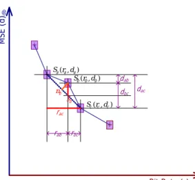
(26) MSE (d)db. Chapter 3. Rate-Distortion Optimization of SVC Bitstream Extraction. +. +. Sa (ra , da ) S (r , d ) + b b b nb. εb. dbc. dac. + Sc (rc , dc ). rac rab. dab. +. rbc. Bit Rate (r)Kb/s. Figure 3.1: Measuring components of the deviation from convexity of a NAL cluster along an SVC R-D curve. extraction paths with slightly non-convex R-D curves may have better performance than the ones with convex R-D curves. In those cases, we should choose a near-optimal extraction path that has the smallest area underneath its R-D curve while the deviation from convexity of the R-D curve falls below a tolerance limit. Criterion 3 Tolerance Limit for Deviation from Convexity. An SVC extraction path can be considered as near optimal if and only if the deviation from convexity ζ of its R-D curve at any refinement step (as defined by the following formula) lies within a specified tolerance limit and the total underlying area of its R-D curve is minimum among all the satisfying paths. ζ(Sb ) ,. b. rac. =. rac dab − rab dac 2 rac. (3.4). Figure 3.1 illustrates the quantities appeared in Equation 3.4 and offers a physical interpretation of the measurement ζ. As shown in the figure, ζ(Sb ) is a ratio between the increment in MSE distortion. b. and the increment in bit rate rac within a non-. convex segment [Sa , Sb , Sc ] of an R-D curve. This ratio must be small in order for the deviation from convexity to be deemed acceptable. This is particularly true at the early refinement steps, in which the increases in bit rates are moderate while the decreases in distortion measures are steep. Only minute deviation of convexity can be tolerated in those early steps. -15-.

(27) CHAPTER 4. Searching for Optimal Extraction Paths. An exhaustive search can be used to find the optimal extraction path by decoding all scalable layers and measuring R-D slope of every refinement step. While R-D performance of all possible combinations of extraction paths are computed, it is easy to find out which one not only maintains its convexity but also has minimal underlying area for the corresponding R-D curve by exhaustively comparing. However, the decoding process of all S(L, T ) embedded in an SVC bitstream is extremely time consuming. Hence, the number of scalable layers required for decoding through searching processes is treated as complexity measure in this thesis. In the following paragraphs, we introduce graphical tools to model the process of successively refined bitstream extraction and then design more efficient search strategies for searching optimal extraction path.. 4.1. Graphical Tools. To aid our search for the optimal extraction path of an successively refined SVC bitstream, we developed two graphical tools and named them, the R-D mesh and the trellis diagram of the bitstream. Following paragraphs explain the essence and the uses of these tools. -16-.

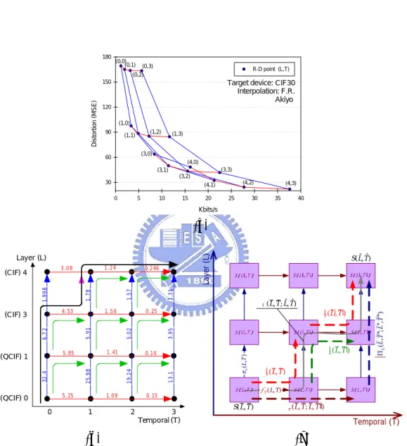
(28) Chapter 4. Searching for Optimal Extraction Paths For the sake of examining the R-D improvement contributed by different refinement steps, we displayed in a single diagram all the piecewise-linear R-D curves of the extraction paths produced by successive refinement of an SVC bitstream. The R-D curves form a mesh, which we call the R-D mesh of the SVC bitstream. Every node in the R-D mesh represents a scalable layer representation S(L, T ) in the bitstream and is labeled explicitly by its layer L and temporal T identifiers. The coordinates (r, d) of the node represent the bit rate and the distortion of S(L, T ), which is decoded and interpolated to fit the display format of target devices to measure viewing quality. Every line segment in the mesh, on the other hand, corresponds to a refinement step π in either L or T dimension: πL (L, T ) : S(L, T ) → S(L0 , T ). (4.1a). πT (L, T ) : S(L, T ) → S(L, T 0 ). (4.1b). where L0 and T 0 denote the subsequent spatial/CGS and temporal layers. The slope of each segment equals to the negation of the R-D improvement contributed by the corresponding refinement step. Similarly, for the sake of exhibiting all possible extraction paths of an SVC bitstream, we superimpose them onto a grid of all scalable layer representations S(L, T ) embedded in the bitstream, and call the composite diagram, the trellis diagram of the SVC bitstream. Again, every node and edge in the trellis diagram represents a scalable layer representation and a refinement step respectively. In the trellis diagram, however, the coordinates of the nodes are their identifier values (L, T ) while the edges are explicitly labeled with the R-D improvement γL (L, T ) and γT (L, T ) offered by the corresponding refinement steps. Plausible extraction paths and their segments are also drawn on top of the trellis diagram to illustrate the process of searching for the optimal path. Figure 3.1 displays the R-D mesh and the trellis diagram of the Aikyo test sequence. Box (a) shows the R-D mesh; box (b) shows the trellis diagram, and box (c) gives a conceptual rendering of a simple trellis diagram. These tools are used in the rest of this thesis both to expound the search strategies and to interpret the experiment results.. -17-.

(29) Chapter 4. Searching for Optimal Extraction Paths. 180. (0,0) (0,1). (0,3). R-D point (L,T). (0,2). Target device: CIF30 Interpolation: F.R. Akiyo. Distortion (MSE). 150. 120 (1,0) 90. (1,2). (1,1). (1,3). (3,0). 60. (4,0) (3,3). (3,1) (3,2) 30. (4,2). (4,1) 0. 5. 10. 15. 20. 25. (4,3). 30. 35. 40. Kbits/s. (a) 1.24. 1.56. 0. 1.31. Π′T ( L′, T ′) S ( L ′ ,T ). S ( L ′ ,T ′). S ( L ′ , T ′′ ). Π′L ( L , T ′) Π ′T ( L , T ) S ( L ,T ). 0. 15. 2. S ( L ′′ , T ′′ ). ℘ ( L , T ; Lˆ , Tˆ ) Π. 0.16. 1.09. 1. S ( L ′′ , T ′ ). S ( L ′′ , T ). 13.1. 25.98. 32.4 5. 25. (QCIF) 0. 5.02 1. 41. 5. 85. (QCIF) 1. S ( Lˆ , Tˆ ). 0. 25. 19.24. 6.7 2. 5.91. 4. 53. (CIF) 3. 3.95. 1.78. 1.998. (CIF) 4. 0.246. 1.57. 3.08. Layer (L). Layer (L). S (L,T ). 3 Temporal (T). π T ( L, T ). S ( L ,T ′). S ( L ,T ′′ ). ΠT ( L , T ; L , T ′′). Temporal (T). (b). (c). Figure 4.1: R-D mesh and trellis diagram of an SVC test bitstream, Akiyo (CIF30). -18-.

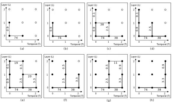
(30) Chapter 4. Searching for Optimal Extraction Paths. 4.2. Search Strategy. 4.2.1. Dynamic Programming Algorithm. Based on trellis diagrams, we can design search strategies to discover extraction paths who have maintained the convexity for corresponding R-D curve (named as convex extraction paths) by examining R-D performance of every refinement step from base unit to target layer. After that, the underlying area of their R-D curve can be computed and compared to find the optimal extraction path. Thinking of this process, dynamic programming algorithm, which is the most classic optimization method, is an available search strategy that can surely find the optimal extraction path if it is existent. Utilizing dynamic programming to discover convex extraction paths is composed of two iterative phases: 1. The trellis grows in both spatial/CGS and temporal dimensions from each existent path until the paths reach target layer. The word "grow" means to decode subsequent scalable layers with one more spatial/CGS or temporal enhancement layer and evaluate the incremental R-D ratio. 2. Non-convex paths are figured out and pruned at each stage by comparing RD performance with those of previous refinement step. Due to transitivity of inequality (A > B ∧ B > C ⇒ A > B > C), the convexity of extraction paths can be maintained even if the incremental R-D performance only compared with preceding one stage while pruning. After all paths reaching the target scalable layer, the maintained paths are candidates of optimal extraction path. Finally, the one with the smallest total area underneath its R-D curve is the optimal extraction path. Figure 4.2 shows an example of process using dynamic programming algorithm as search strategy to find the optimal extraction path. Each box in figure illustrates a step. In these trellis diagrams, we denote block nodes as scalable layers that have been decoded and white ones as those not have been decoded. Moreover, the refinement steps depicted as thin edges to represent that their R-D information are evaluated. If R-D curve of the extended path is convex, it would be maintained and depicted as broader edge. Otherwise, the edge would be pruned and eliminated. The process is described below.. -19-.

(31) Chapter 4. Searching for Optimal Extraction Paths. Layer (L) 2. 1. 1. 1. Layer (L) 2. (e). 74 0. 0.9. 2.5 0.5. 0. 38 1. 1. 2.5. 2.5 0. 2 Temporal (T). 2 Temporal (T). 2 Temporal (T). 2. 1. 3.3. 2.5 38 1. 38 1. (d). 11. 0.5. 0.5. 0.1 0.9. 74 0. 74 0. Layer (L). 2. 1. 20. 2 Temporal (T). Layer (L). 2. 19. 0. 38 1. (c). Layer (L). 1. 74 0. (b). Layer (L). 0. 2 Temporal (T). 0.9. 1. (a). 2. 0. 74 0. 74 0. (f). 38 1. 3.3. 2 Temporal (T). 3.3. 1. 0.9. 0. 74 0. 3.3. 0. 1. 38 0.9. 0.9. 0.9. 0.1. 2. 2.5. Layer (L). 2. 0.1. Layer (L). 2 Temporal (T). 0. 74 0. (g). 38 1. 2 Temporal (T). (h). Figure 4.2: Example: using dynamic programming algorithm to find the optimal extraction path.. Step 1 ) Trellis starts from base unit and grows in both L and T dimensions as shown in Figure 4.2(a). Step 2 ) These two paths are both kept as shown in Figure 4.2(b). Step 3 ) Next iteration, trellises grow in two dimensions from existent two paths as shown in Figure 4.2(c). Step 4 ) Pruned πT (1, 0) since it can not construct a convex extraction path (0.9 < 38). The other three edges become broader to represent the paths are maintained as shown in Figure 4.2(d). Step 5 ) Trellises grow from existent three paths as shown in Figure 4.2(e). Step 6 ) Pruned πT (1, 1) since γL (0, 1) < γT (1, 1) (as shown in Figure 4.2(e), 2.5 < 20) and pruned the path with πT (2, 0) due to γL (1, 0) < γT (2, 0). The other paths are kept as shown in Figure 4.2(f). Step 7 ) Trellises grows in only L or T dimension because each of existent paths had reached their target layer in another dimension as shown in Figure 4.2(g). Step 8 ) Pruned the path with πT (2, 1) due to γL (1, 1) < γT (2, 1). After four grew and pruned iterations, all paths reach target layer in both L and T and the process stop. In this example, the process left only one convex extraction path in the end, which -20-.

(32) Chapter 4. Searching for Optimal Extraction Paths is the optimal extraction path. Although dynamic programming algorithm can ensure finding all convex extraction paths, its computational complexity is still considerable. It works better than exhaustive search since some paths may be pruned without evaluation and even some nodes (scalable layers) may be skipped without decoding. However, as we can see in Figure 4.2, the gain over exhaustive search is insignificant in case that the size of trellis diagrams are small because almost every nodes are required for decoding. On the contrary, if the number of scalable layers is large, the complexity of dynamic programming algorithm grows exponentially. Therefore, we need more aggressive pruning rules in a search strategy to discover convex extraction paths.. 4.2.2. Greedy Heuristic Scheme. Since the efficiency of dynamic programming is not much better than exhaustive search, we propose a greedy heuristic scheme to tackle the problem. The main concept of "greedy" scheme is that every refinement step of extraction path is decided at every stage without looking ahead. This approach also consists of two iterative phases: 1. The same as dynamic programming algorithm, trellises grow in both spatial/CGS and temporal dimensions from existent paths. 2. The refinement step with worse incremental R-D improvement is pruned and only one path would be kept at each stage. In other words, the greedy heuristic scheme is performed as steepest-descent method. While the path reaching target layer in any dimension, no more scalable layers are needed to decode and evaluate since there is only one choice for further refinement steps. For instance, Figure 4.3 presents a process using greedy heuristic scheme as search strategy to find the optimal extraction path. The process is described below. Step 1 ) Trellis starts from base unit and grows in both L and T dimensions as shown in Figure 4.3(a). Step 2 ) Since γL (0, 0) is worse than γT (0, 0) (as shown in Figure 4.3(a), 0.9 < 74), πL (0, 0) is pruned yet only πT (0, 0) is kept as shown in Figure 4.3(b). Step 3 ) Trellis grows from the only one existent path as shown in Figure 4.3(c). Step 4 ) πL (0, 1) is pruned yet πT (0, 1) is kept due to γL (0, 1) < γT (0, 1). As shown -21-.

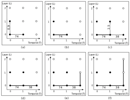
(33) Chapter 4. Searching for Optimal Extraction Paths Layer (L). Layer (L). Layer (L). 2. 2. 1. 1. 1. 0.9. 2.5. 2. 0. 0. 74 0. 1. 2 Temporal (T). 0. 74 0. 1. (a). 2 Temporal (T). Layer (L). Layer (L). 2. 2. 1. 1. 1. 74. 38 1. 2 Temporal (T). (d). 0. 74 0. 2 Temporal (T). (c). 2. 0. 38 1. (b). Layer (L). 0. 74 0. 38 1. (e). 2 Temporal (T). 0. 74 0. 38 1. 2 Temporal (T). (f). Figure 4.3: Example: using greedy heuristic scheme to find the optimal extraction path.. in Figure 4.3(d), the existent path reach target layer in temporal dimension. Step 5 ) No more scalable layers are needed to decode. The refinement step in spatial dimension is included in the path as shown in Figure 4.3(e). Step 6 ) Again, no more scalable layers are needed to decode. The path include the left refinement step in spatial dimension thus reach the target layer in both dimensions and end the process as shown in Figure 4.3(f). The greedy heuristic scheme presents significant complexity reduction about 50% or more. Even number of scalable layers is small, almost half of them not have to be decoded [Figure 4.3 (f)]. Moreover, since always only one path is maintained through whole process, the complexity of greedy heuristic scheme grows linearly while the number of scalable layers increasing. Intuitively speaking, this approach seems no guarantee of optimality of solution. Its pruning rules are designed neither with verification of R-D convexity nor with comparison of underlying area for corresponding R-D curve. However, empirical finding from our experimental results exposes that greedy heuristic scheme often can obtain the optimal extraction paths or reveal a path with comparable R-D performance. For instance, the previous example in Figure 4.3 obtained the same answer as the optimal extraction path produced by dynamic programming algorithm in Figure 4.2. The -22-.

(34) Chapter 4. Searching for Optimal Extraction Paths surprisingly good performance of this scheme is theoretically analyzed in next section.. 4.3. Analysis of Greedy Heuristic Scheme. We analyze the effectiveness of greedy heuristic scheme based on studying properties of trellis diagrams. Started with convex segments across single trellis and along one dimension, we discovered some satisfying conditions to construct convex extraction paths or even optimal extraction paths.. 4.3.1. Convex Segments and Global Condition. All R-D convex extraction paths can be constructed from two elementary types of R-D convex segments as shown in Figure 3.1 (c): 1. Intra-trellis (local) convex segments, which consist of two refinement steps, one of each in L and T dimensions: Π0L (L, T ) = πL (L, T ) k πT (L0 , T ). (4.2a). Π0T (L, T ) = πT (L, T ) k πL (L, T 0 ). (4.2b). Each of these convex segments traverses a single four-node trellis. 2. Inter-trellis (global) convex segments, which also consist of two refinement steps, both of them in either L or T dimensions: ΠL (L, T ; L00 , T ) : πL (L, T ) k πL (L0 , T ). (4.3a). ΠT (L, T ; L, T 00 ) : πT (L, T ) k πT (L, T 0 ). (4.3b). Each of these inter-trellis convex segments traverses two connected trellises in L or T dimensions. The existence of intra-trellis segments Π0L and Π0T cannot be controlled directly by the setting of SVC encoding process. However, they can be verified by comparing the R-D improvement γL or γT of their first refinement steps {πL , πT } against the R-D. -23-.

(35) Chapter 4. Searching for Optimal Extraction Paths improvement Γ0 of the intra-trellis segments {Π0L , Π0T }: Π0L (L, T ) exists iff γL (L, T ) ≥ Γ0 (L, T ). (4.4a). Π0T (L, T ) exists iff γT (L, T ) ≥ Γ0 (L, T ). (4.4b). The existence of inter-trellis segments ΠL and ΠT , nonetheless, can be manipulated indirectly by the setting of quantization parameter QP, inter-layer dependencies and temporal dependencies among the SVC coding layers. In fact, as mentioned in Chapter 5, R-D convex paths in L and T dimensions may exist at every L and T values if parameter setting satisfy certain constraints for well-adapted SVC encoding. The discovery of this correlation between SVC encoder setting and decoder (extraction) operation is a major contribution of this thesis. Here, since the existence of convex R-D curves in every spatial/quality and temporal layer was essential for forming convex extraction paths, we referred it as the global condition.. 4.3.2. Strong Local Conditions. The simplest composition of trellis diagram is single four-node trellis. We looked into four-node trellises to figure out the conditions for existence of intra-trellis (local) convex segments. We defined that it is strong local condition satisfied if one and only one intratrellis convex segment exists in every trellis. This situation arises when there is a clear domination of R-D improvements in either L or T dimension: Only Π0L (L, T ) exists iff min (γL (L, T ) , γL (L, T 0 )) > max (γT (L, T ) , γT (L0 , T )) (4.5a) Only Π0T (L, T ) exists iff min (γT (L, T ) , γT (L0 , T )) > max (γL (L, T ) , γL (L, T 0 )) (4.5b) With this strong local condition and the global condition, the search for the optimal extraction path can be perfectly performed using greedy heuristic scheme (steepest descent method). This simple search strategy is feasible because there exists a unique ˆ Tˆ) convex extraction path between the base unit S(L, T ) and any target layer S(L, if both strong local and global conditions of R-D performance are satisfied in an SVC bitstream. Figure 4.4 illustrates a typical example. Notice that the intra-trellis convex -24-.

(36) Chapter 4. Searching for Optimal Extraction Paths Layer (L). S ( Lˆ ,Tˆ ). 3. 2. 1. 0. S( L, T ) 0. 1. 2. 3 Temporal (T). Figure 4.4: A trellis diagram with convex segments satisfying strong intra-trellis (local) and inter-trellis (global) R-D conditions. segments Π0L and Π0T tend to concentrate in two separate regions of the trellis diagram: Π0L (drawn as magenta arrows) gathers in the upper-left corner while Π0T (drawn as green arrows) gathers in the lower-right corner. Both types of convex segments bend their paths towards the boundary that separates the two regions. This is owing to the contradiction between global and strong local conditions. The inequalities in Equations 4.5a and 4.5b eliminate the chance for Π0L (a magenta arrow) to appear underneath or to the right of Π0T (a green arrow). The boundary between the two regions defines a convex and optimal extraction path (with maximum convexity and minimum underlying area) of the SVC bitstream because any other extraction path between the same end points would inevitably traverse at least one intra-trellis non-convex segment and thus yield ˆ Tˆ) through any a worse R-D performance. Hence, the traversal from S(L, T ) to S(L, four-node trellis would follow the intra-trellis convex segments, which can be reduced as choosing steepest descent refinement steps at any steps.. 4.3.3. Weak Local Conditions. Among all the R-D trellises of an SVC bitstream, some of them contain R-D convex segments but lack a clear domination of R-D performance in either L or T dimension. We named it weak intra-trellis (local) condition if R-D performance of the four refinement steps in four-node trellis satisfies Equations 4.4a and 4.4b but not Equations 4.5a. -25-.

(37) Chapter 4. Searching for Optimal Extraction Paths Layer (L). S ( Lˆ ,Tˆ ). 3. 2. 1. 0. S (L, T ) 0. 1. 2. 3 Temporal (T). Figure 4.5: A trellis diagram with convex segments satisfying weak intra-trellis (local) and inter-trellis (global) R-D conditions. and 4.5b. In these cases, both Π0L and Π0T exist in each of these trellises. The existence of multiple convex segments in one or more trellises revokes the unique existence of convex extraction path. Hence, the greedy heuristic scheme could not promise to fine the optimal extraction path. However, the difference in underlying area of two convex R-D curves in single four-node trellis is usually insignificant. Furthermore, the trellises that satisfied weak local condition almost appeared along the boundary between two regions of strong local conditional trellises empirically. Figure 4.5 shows an example of this situation. As a result, all the convex extraction paths may have similar underlying area of R-D curves and the greedy heuristic scheme can find one of them. Even though it may not be the optimal extraction path, it would have similar R-D performance.. 4.3.4. Fractional Violation of Local Conditions. In some rare cases (when a subjective measures such as the mean opinion scores is used to quantify playback picture quality), the local R-D condition (i.e. the existence of intra-trellis R-D convex segments) may fail to be upheld. As a result, no convex exˆ Tˆ) pairs. A near-optimal extraction traction path exists between some S(L, T ) and S(L, path with a slightly non-convex R-D curve [Section 3.3] may have to be accepted as a substitute instead. In the search for the near-optimal extraction path, extraction path segments with R-D curves that contain slight deviation from convexity [Criterion 3] are included into consideration. Figure 4.6 provides an example that contains a violation -26-.

(38) Chapter 4. Searching for Optimal Extraction Paths Layer (L). Dis tortion. S ( Lˆ , Tˆ ). (0,0 ). 2 (1,0) (0 ,1). (2,0). 1 (0,2) (1,1). (2,1). 0 (1,2). (2 ,2). Rate. (a). S(L , T ) 0. 1. 2 Temporal (T). (b). Figure 4.6: R-D mesh and trellis diagram of an SVC bitstream with fractional violation of intra-trellis (local) R-D conditions. of local R-D condition in the lower-left trellis. A slightly non-convex segment Π0T (0, 0) shown as a dashed magenta arrow would not be pruned during searching. In these cases, the greedy heuristic scheme generally has no promise to find the optimal/near-optimal extraction paths. However, the violation of local conditions rarely occurred.. 4.4. Summary. In this chapter, we exploited dynamic programming algorithm and proposed greedy heuristic scheme for searching optimal extraction paths. We reveal the effectiveness and limit of the greedy heuristic scheme by analyzing proposed R-D trellis diagrams. The global and local conditions promise the existence of optimal extraction paths. To satisfy the global and strong local condition ensures that the optimal extraction path can be found using efficient greedy heuristic scheme. The local condition depends heavily on video contents and local R-D variations causing by measure schemes or interpolation approaches, while global condition relies on well-adapted temporal and inter-layer dependencies. In next chapter, we introduce proper settings of encoding parameters to produce well-adapted SVC bitstreams for efficient searching optimal extraction paths.. -27-.

(39) CHAPTER 5. Production of Well-adapted SVC Bitstreams. The second part of our investigation aims at establishing the necessary criteria that must be satisfied during SVC encoding in order to guarantee the existence of optimal extraction paths. Specifically, we examined the combined effects of quantization parameter (QP) setting and inter-layer dependence relations on the R-D performance of an SVC bitstream.. 5.1. Settings of Quantization Parameters. One important issue in SVC encoding is to determine the QP values for spatial and quality layers so that the resulting bitstream can meet the predefined quality or bit rate constraints. While the application requirements seem to be arbitrary, it should be noted that improper QP settings may produce ill-formed R-D performance and redundant representations. To this end, we proposed two criteria for evaluating the properness of QP assignment when combined scalability is in use. Criterion 4 Monotonic Decrease in QP Value for Successive Refinement. In a given spatial resolution, the QP value should decrease monotonically from one quality layer to the next in order to successively refine texture information. -28-.

(40) Chapter 5. Production of Well-adapted SVC Bitstreams Criterion 5 Elimination of Redundant Representations. For different spatial resolutions, the high-resolution layers should have higher fidelity than the spatially interpolated low-resolution layers in order to eliminate redundant representations. Criterion 4 requires the picture quality to be successively refined as the size of the bitstream increases by extracting more quality layers. Criterion 5 further prohibits redundant layers from being encoded. We say that a high-resolution layer is redundant if there exists another low-resolution layer that can provide the same or even higher fidelity by spatial interpolation. Clearly, such redundancy should be detected and removed during SVC encoding. In particular, the two criteria specify only the relative QP level among the spatial and quality layers–i.e., the exact values still need to be decided by the intended applications. For instance, by focusing our attention on mobile streaming applications, in our experiments the PSNR of spatial/quality layers is set to fall between 27dB and 35dB. Exhaustive encoding was carried out off-line to obtain the QP values for different test sequences.. 5.2. Settings of Inter-layer Dependencies. In our efforts to devise efficient search strategies for optimal/near-optimal extraction paths, we discovered that the global condition can be satisfied by maintaining the convexity of R-D curves across spatial/quality and temporal layers during SVC encoding. With hierarchical and dyadic temporal dependencies, the cascading QP assignment in current JSVM [11] can already make the R-D curves across temporal layers convex in most cases, especially when MSE is used for distortion measure. This is because higher temporal layers are coded with larger QP values, which inherently leads to diminishing R-D improvement with increasing temporal level. On the other hand, among the spatial and quality layers, the convexity of their R-D curves can be guaranteed by satisfying the following criterion. Criterion 6 Convexity of Rate-Distortion Curves across Spatial and Quality Layers. An SVC encoder should produce an SVC bitstream according to a well-adapted interlayer (spatial and quality) dependence relation that ensures every successive refinement of scalable layer representations exhibits a monotonic decrease in MSE dis-29-.

(41) Chapter 5. Production of Well-adapted SVC Bitstreams. Distortion at target resolution. A B C. D. E(2). E (1). Setting 1. Setting 2. E. E. D. D. C. C. B. B. A. A. Rate. Figure 5.1: R-D performance of SVC bitstreams with different inter-layer dependency settings. Labels A, B, C, D, and E denote five coding layers of different SNR levels with E being the target layer for reconstruction.. tortion d(Li , Tb) > d(Li+1 , Tb) as well as a monotonic decrease of R-D improvement γL (Li , Tb) > γL (Li+1 , Tb) > 0.. This criterion forbids the slope of the R-D curves to steepen (or equivalently their R-D improvement to rise) as a viewing device takes in a sequence of coding layers in successive refinement steps. Its practical implication can be explained using an example shown in Figure 5.1. In the example, each layer (from B to E) in Setting #1 depends on its previous layer; hence, the reconstruction of layer E requires the decoding of all its dependent layers from A to D. However, because the R-D improvement produced by D is not as good as the one produced by E, Setting #1 cannot maintain the R-D convexity. In contrast, Setting #2, which links C directly to E by skipping D, is a well-adapted dependency setting. We must advise readers to exercise caution when they try to set up a well-adapted inter-layer dependence relation because the adaptation can easily be overdone. In Figure 5.1, although Setting #2 (which ensures R-D convexity along the spatial/quality dimension) produces a better R-D performance for a single viewing device even if it takes layer E in one moment and layer D in another, Setting #1 (which fails to maintain R-D convexity) consumes less bandwidth when it comes to serving two viewing devices existing in the same network. This observation confirms a well-known fact that the SVC coding gain over simulcasting is at the cost of the R-D performance of individual layers. Our advice of caution can be summarized in the following proposition. Proposition 1 Minimal Adaptation of Successive Inter-layer Dependencies. An SVC encoder should choose a successive inter-layer dependence relation, which usually pro-30-.

(42) Chapter 5. Production of Well-adapted SVC Bitstreams duces the lowest bit rates, to be the default dependency setting. The dependence relation should only be modified at the refinement steps that produce non-convex R-D improvements. At those refinement steps, the reference layers should be chosen to be the nearest spatial/quality layers that can produce convex R-D improvements. Again using the example in Figure 5.1, a proper adjustment of inter-layer dependencies is to make layer E depend on layer C rather than layer B. This minimal adjustment of inter-layer dependence relations shall only cause a small increase in the total data rate of the SVC bitstream. We would like to emphasize that such strategy is to ensure the global condition rather than to optimize the R-D performance of individual layers. For the later case, readers are referred to the paper by Yao and Li [17] for more complete discussion.. -31-.

(43) CHAPTER 6. Experiments. 6.1. Implementation of Well-adapted SVC Bitstream. Having described our criteria for well-adapted bitstreams, this section further presents a practical approach for generating well-adapted inter-layer dependencies.. 6.1.1. Prediction of R-D Convexity. To predict the R-D performance of SVC along the spatial/quality dimension, one effective approach is to evenly add 10% or more redundancies1 to the R-D points of H.264/AVC [13]. The results generally hold when multi-loop encoder control and fixedquality configurations are used [6][13]. Moreover, the predictability remains valid with bottom-up encoding process [11] after taking into consideration that the enhancement layers usually suffer more coding efficiency losses than the base layer. The observations enable us to predict the R-D convexity of SVC without the need of exhaustive encoding. 1. Comparing with the single layer coding, the coding efficiency loss of SVC is generally proportional to the number of coding layers. In some cases, the R-D gap between H.264/AVC and SVC can be much greater than 10%.. -32-.

(44) 37 36 35 34 33 32 31 30 29 28 27 26 25 24 23 22 21 20 19. 36. Mobile. Foreman. 35. B1. A2'. A2'. B1. 34 33. B0. A1'. PSNR-Y (CIF). PSNR-Y (CIF). Chapter 6. Experiments. A0'. A1. A2. 31. A1'. B0. 30 29. A2. 28. SVC 1:(A0,A1,A2,B0,B1) SVC 2:(A0,A1,B0,B1) SVC 3:(A0,B0,B1) AVC CIF AVC QCIF AVC QCIFtoCIF (Interpolation). A0. 32. SVC 1:(A0,A1,A2,B0,B1) SVC 2:(A0,A1,B0,B1) SVC 3:(A0,B0,B1) AVC CIF AVC QICF AVC QCIFtoCIF (Interpolation). A1. 27. A0'. 26 A0. 25 24. 0. 200. 400. 600. 800. 1000. 1200. 1400. 1600. 0. 50. 100. 150. Kbits/s. 200. 250. 300. Kbits/s. (a). (b). Figure 6.1: Comparison of SVC dependency settings: (a) Mobile and (b) Foreman. The results were produced with bottom-up encoding process and fixed-quality configurations.. For validation, several SVC bitstreams, each corresponds to one of the following dependency settings, were encoded using bottom-up encoder control and fixed-quality configurations. In particular, Setting #1 denotes the default dependency setting (which yields a minimal total bit rate), whereas Settings #2 and #3 adapt the default setting by merely changing the reference layer of layer B0. The R-D performances of these dependency settings are compared with that of H.264/AVC in Figure 6.1. • Setting #1: (QCIF A0←A1←A2), (CIF A2←B0←B1). (Default Setting) • Setting #2: (QCIF A0←A1←A2), (CIF A1←B0←B1). • Setting #3: (QCIF A0←A1←A2), (CIF A0←B0←B1). Looking at the R-D points of H.264/AVC in Figure 6.1, one can readily predict that Setting #3 would be a well-adapted setting for Mobile sequence, and the prediction was confirmed by the corresponding SVC R-D curve. Likewise, in Foreman sequence, both Settings #2 and #3 are likely to ensure R-D convexity. Although Setting #3 has better R-D performance, we choose Setting #2 because, as will be seen in the next section, the increase in total bit rate is minimized. In Figure 6.2 we further present the results with fixed-rate configurations, in which the quality (and the QP) of each layer is not fixed; rather, the cumulative rate to each layer is kept constant regardless of dependency settings. Comparing with the H.264/AVC, the coding efficiency loss of SVC can be seen from the drop of R-D curves. Similar to the bit rate increase in fixed-quality configurations, the distribution of PSNR drops helps to predict the R-D convexity of SVC. From Figure 6.2, we obtain exactly -33-.

(45) 36. 37 36 35 34 33 32 31 30 29 28 27 26 25 24 23 22 21 20 19. Mobile. Foreman. 35. B1. A2'. A2'. B1. 34 33 A1'. B0. A0'. A1. SVC 1:(A0,A1,A2,B0,B1) SVC 2:(A0,A1,B0,B1) SVC 3:(A0,B0,B1) AVC CIF AVC QCIF AVC QCIFtoCIF (Interpolation). A2. PSNR-Y (CIF). PSNR-Y (CIF). Chapter 6. Experiments. 32 31. A1'. B0. 30 29. A2. 28 27. A0'. 26. SVC 1:(A0,A1,A2,B0,B1) SVC 2:(A0,A1,B0,B1) SVC 3:(A0,B0,B1) AVC CIF AVC QCIF AVC QCIFtoCIF (Interpolation). A1. A0. 25. A0. 24 0. 200. 400. 600. 800. 1000. 1200. 1400. 0. 1600. 50. 100. 150. 200. 250. 300. Kbits/s. Kbits/s. (a). (b). Figure 6.2: Comparison of SVC dependency settings: (a) Mobile and (b) Foreman. The results were produced with bottom-up encoding process and fixed-rate configurations.. the same dependency settings as with fixed-quality configurations. Interestingly, in Foreman sequence there is a “bump” in the R-D curve with Setting #1. This is because the QP value of layer B0 is improperly chosen to meet the bit rate constraint. The result stresses the importance of proper QP settings. The preceding discussions assume the availability of H.264/AVC R-D points. The assumption does not generally hold unless each layer is pre-encoded with H.264/AVC. Collecting these R-D data is indeed time-consuming, but performing exhaustive SVC encoding is even worse. In addition, in our approach the R-D convexity is guaranteed only at full frame rate. Nevertheless, the global condition requires R-D convexity at all possible frame rates. We have found empirically that the convexity at full frame rate would also likely to ensure the convexity at lower frame rates. After all, the R-D behavior at full frame rate represents the average performance of all video frames.. 6.1.2. Degradation in Coding Efficiency. The previous section has analyzed the SVC R-D convexity under various dependency settings. We now turn our attention to the overall coding efficiency, which is characterized by the total bit rate of an SVC bitstream. As described previously, long-term inter-layer reference may be needed for the sake of R-D convexity. It is natural then to question whether and to what extent the total bit rate will increase. The answers can be found by the comparison shown in Figure 6.3. From there it can be seen that the well-adapted dependency settings (Setting #2 for Foreman; Setting #3 for Mobile) -34-.

(46) Chapter 6. Experiments. 135 Setting 1 Setting 2 Setting 3. Normalized Total Bit Rate (%). 130 125 120 115 110 105 100 95 Foreman-FQ. Foreman-FR. Mobile-FQ. Mobile-FR. Sequences -Approach. Figure 6.3: Comparison of total bit rate for different dependence settings. Fixedquality (FQ) and fixed-rate (FR) configurations were used.. incur, on average, 15∼20% bit rate increase in comparison with Setting #1 (default setting). The penalty arises mostly because layers A1 and A2 are not utilized for the inter-layer prediction of layer B0 in Settings #2 and #3.. 6.2. Analysis of Optimal Extraction Paths. In this section we present a detailed analysis on the optimal extraction paths in regard to the following factors. The analysis is to understand how these factors may affect the choice of optimal extraction paths. • Video Contents: Static vs. Motion. • Device Types: QCIF@30/15Hz, CIF@30/15Hz, and 4CIF@30/15Hz. • Distortion Measures: Mean Squared Error vs. Mean Opinion Score. • Temporal Interpolations: Frame Replication (F.R.) vs. B_Direct_16x16 (B.Direct). Table 6.1 lists our testing conditions, in which the QP assignments and the interlayer dependence settings comply with the guidelines in Chapter 5. To simulate the actual use of SVC, extracted videos were interpolated to the highest spatiotemporal resolutions available on all viewing devices. The interpolation was accomplished by the standard-compliant spatial filtering [11], followed by frame replication (F.R.) or motion field estimation (B.Direct). While sophisticated interpolation techniques could be used, we chose the straightforward implementation because of its simplicity and popularity. In addition, in the experiments comparing subjective and objective distortion measures, we adopted the VQM software [1][10] to predict subjective quality. -35-.