Modeling, analysis, simulation and control of semiconductor manufacturing systems: a generalized stochastic colored timed Petri net approach

Modeling, Analysis, Simulation and Control of Semiconductor Manufacturing

Systems: A Generalized Stochastic Colored Timed Petri Net Approach

Ming-Hung Lin and Li-Chen F’u

Dept. of Computer Science and Information Engineering, National Taiwan University,

Taipei, Taiwan, R.0.C

E-mail: lichen@ccms.ntu.edu.tw

ABSTRACT

In this paper, a generalized stochastic colored timed Petri net(GSCTPN) is used t o model an IC wafer fabrication system. There are two major sub-models: Process-Flow Model and Transportation Model. There are two different automated guided vehicle systems, namely, Interbay system and Intrabay system. For multiple-load and variable-speed AGV system, we em- bed a simple motion-planning rule and introduce a col- lision avoidance strategy in model to solve the variable speed and traffic jam problems of vehicles. The simple control policies for AGV’s visiting and AGV’s routing are discussed. The heuristic rules for lot release and lot scheduling are also studied. To obtain performance measures, simulation is used. To show the promising potential of the proposed work, a real-word IC wafer fabrication system is used as a target plant layout for implementation.

1 Introduction

The previous works in applying Petri nets t o IC wafer fabrication are discussed below. Modeling, analysis, simulation, scheduling, and control of semiconductor manufacturing systems was performed by using Petri nets in [I]. It also serves as a good tutorial paper. Jan- neck [2] presents the modeling a die bonder with Petri nets. Xiong et a2.[3] propose and evaluate two Petri-

net based hybrid heuristic search strategies and their applications t o semiconductor test facility scheduling. In [4], hybrid Petri nets are presented as tools for mod- eling and simulation of semiconductor manufacturing systems. The colored timed Petri net(CTPN) is used t o model the furnace in IC wafer fabrication, based on CTPN, the dynamic behaviors of the furnace can be emulated [5]. Jeng et al.[G] report a project of applying Petri net methodologies t o dctailed modeling, qualita- tive analysis, and performance evaluation of the etch- ing area in an IC wafer fabrication system located in Taiwan’s Hsinchu Science Based Industrial Park.

In this paper, a generalized stochastic colored timed Petri net(GSCTPN) model is built to model the detailed behaviors of an IC wafer fabrication sys- tem. Some control policies generated based on that GSCTPN model are t o optimize some a priori assigned performance criterion. The plant layout and process-

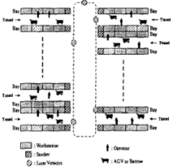
Figure 1: Physical Layout

ing steps are similar t o that in [l, 61. Different from the model proposed in [l, 61, the present work introduces a GSCTPN modeling of a general IC wafer fabrication system. The result net model solves the 711~ng’7 net modeling of reentrant processing problem and contains fewer of places and transitions; especially, including two different multiple-load and variable-speed AGV transportation systems. Although the AGV trans- portation system provides us flexibility and economy, it leaves us numerous ways of routing which unfortu- nately gives the control problem a combinatorial fla- vor. The organization of this paper is as follows. Sec- tion 2 describes the overview of IC manufacturing pro- cess and the IC plant layout. Section 3 introduces a GSCTPN Modeling of system. Section 4 describes a performance analysis based on simulation. Section 5 is conclusion.

2 System Description

In general, the machines in an IC wafer fabrication sys- tem are grouped into four functional sections: the pho- tolithography area, the diffusion area, the etching area,

and the thin film area. A processing unit of wafers is called a lot in an IC wafer fabrication. When lots arrive

at the IC factory, they are processed in the previously mentioned four areas. As shown in Fig. 1, an IC plant is a base of tunnels. Machines are placed beside the

tunnels, they are grouped into a bay. In the Interbay

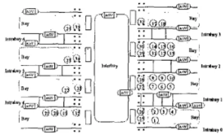
system, The corresponding AGV stops are arranged in location 25-35 as shown in Fig. 2. There is only one single-loop track in the Interbay system. In the In-

Figure 2: Plant Layout

terbay system, AGV that are called loop vehicles can move to any stop in unidirectional. Each stop in Inter- bay system is used as a transit station that transports lots between different bays. We denote the transit sta- tion as Interbay stationorstoker. There are 24 stations divided into 6 types, each of multi-server stations con- sists of several identical pieces of equipment. There are two types of lots associated with different wafer processing flows. One consist,s of 172 operations. The other consists of 148 operations.

3 Generalized Stochastic Colored Timed Petri Net Modeling

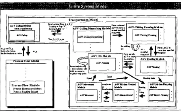
The proposed generalized stochastic colored timed Petri-Net (GSCTPN) extends the framework of the original PN by adding color, time and modular at- tributes to the net. The GSCTPN model contains two major sub-models. One is called Transportation Model, and the other is called Process-Flow Model. 3.1 Modeling for Process Flow

The Process Flow Model can be decomposed into two micro-models, each with different characteristics. One is Process Routing Module and the other is Process Elementary Module. The following are detailed de- scriptions of each of these micro-models.

Process Routing Module

The GSCTPN model we proposed to illustrate the processing flow of each lot type is Process Flow Model. It models the technological precedence constraints for processing lots and provides normally more than one alternative routes t o accomplish the operation process- ing. The essential idea is that, the number of color set is equal to sum of adding total processing-steps for each type of lot. This means that the processing-steps attribute is embedded as colors to the model. For ex- ample, the number of processing steps for type 1 is 172 and that of type 2 is 148. Then, the number of color is 320. Token in color set IC represents that a lot is currently processing a t the k-th step. Moreover, the number of tokens in color set k represents the how many lots currently is at the k-th step.

Figure 3: Process Routing Module

Figure

4:

Process Elementary Module

Process Elementary Module

The Process Elementary Module can be composed of four subnets as shown in Fig. 4, each with differ- ent characteristics. They are, namely, Processing Sub- net, Inspection Subnet, Machine Subnet, and Inspec- tion Machine Subnet. However, the Inspection Subnet and Inspection Machine Subnet has t o be additionally included if wafers need to be inspected. The following are detailed descriptions of each of these subnets.

The essential idea of modeling Processing Subnet is that, before a lot can take up any resource, it must acquire its control right in terms of a token. For ex- ample as shown in Fig. 4, if a lot wants t o move t o the machine Mac-i-j-1 located at the stop

x,

it must get the token of resource place man-i-j-1. Moreover, if the current location where the wafer resides is not the same with that of machine Mac-i-j-1, it is need t o send a signal in the communication place To-2. It invokes an AGV to come to the place where the wafer resides. When the AGV arrives, it proceeds t o load the wafer. The AGV starts to move to the destination place.

Machines may fail, it is very common in IC fabri- cation. In Machine Subnet which is shown in Fig. 4, an operation transition man-i-j-Z-mtbf will be fired pe- riodically according to the fabrication statistics. It is called mean time between faiZure(MTBF). If transition

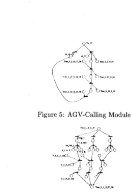
Figure 5: AGV-Calling Module

Figure 6: AGV-Calling Dispatching Module

man-i-j-1-mtbf is fired, intermediate transition man-i- j-1-fa is enable and will be fired immediately. While man-i-j-1-fa is fired, a token leaves from the resources place man-i-j-1

.

The repairing time is called mean time to repair(MTTR). While the time of operation transition man-i-j-l-mttr has passed, the machine re- pair has been completed and a token returns t o place man-i-j-1.

3.2 Modeling for Transportation System The Transportation Model can be decomposed into several micro-models7 each with different characteris- tics. The following are detailed descriptions of each of these micro-models.

AGV-Calling Module

For example as shown in Fig. 5, a lot is located at the stop 5 currently and the next serving station is lo- cated at stop 19. Before the next operation, the com- munication place To-19 is marked to signal AGV and invokes an AGV t o come t o the place where the wafer resides. The stop 19 is located at different'bay, it must be competed with the following steps. First, the com- munication place T o u r L 5 S - 2 7 is marked. It means that wafer will have a tour loading from stop 5 and storing at stop 27. When the AGV arrives, AGV pro- ceeds to load the wafer. Then, the AGV starts t o move t o the Interbay station 27. A token in communication place Tour-L-5-S-27-ok indicates that the transporting tour from 5 to 27 is completed successfully.

AGV-Calling Dispatching Module

There are two considering in AGV-Calling Dispatch- ing Module which is shown in Fig. 6 . One is

Figure 7: AGV-Visiting Planning Module

AGV-Calling Dispatching, the other is precedence con- straints for transporting lots. When a token is in the communication place TourL-53-27, it indicates t h a t a lot transporting to be served. It can be completed with two steps. First, an AGV is selected according t o the dispatching policy. A good dispatching policy can make higher utilization of AGVs. Initially, we as- sume t h a t there are three AGVs in the Intrabay 1. It is shown in Fig. 2. If AGV 1 is selected, the intermediate transition Disp-1 is fired. A token enters the interme- diate place V-LWC. It means that a lot is waiting for AGV 1 t o transport. If the buffer of selected AGV is not full, the resource place V-1-B is marked. The in- termediate transition As-OK-1 is enable and it can be fired.

AGV-Visiting Planning Module

Each multiple-load AGV may have t o reach sev- eral stop points for loading or storing wafers.

A

good visiting planning is need t o solve the traffic jam problems of vehicles. For example, there are eight stops(2,3,4,5,6,7,26,27) in the Intrabay 1. It is shown in Fig. 2. For example as shown in Fig. 7, if the communi- cation place V-1L-5 is marked, it indicates t h a t AGV

1 is need t o arrive at stop 5 for loading a lot. Then, the communication place V-1-To-5 and V-1L-C-5 are both marked. A token in the communication place V-1-To-5 represents t h a t AGV 1 must visit the stop 5. A token in place V-1L-C-5 represents t h a t the goal of AGV 1 at stop 5 is to load a lot. If the communica- tion place V-13-27 is marked, it represents t h a t AGV

1 need t o arrive a t stop 27 for storing. A token in the communication place V-1-To-27 represents t h a t AGV 1 must visit the stop 27. A token in place V-1-S-C-27 denotes t h a t the goal of AGV 1 a t stop 27 is t o store a lot. Furthermore, when the communication place Vi-1-OK has a token, it means t h a t the current visit- ing is finished and proceeds t o next visiting. However, if there are no queues for visiting, the communication place V-1-Idle will be marked. It indicates that AGV 1 is a t idle state.

Figure 8: AGV Routing Module

Figure 9: AGV Routing Module

AGV Routing Module

The basic concept of this model is described as follows. When an AGV needs t o move from the current stop to the next adjacent stop, there are two steps to achieve that. Firstly, it needs to receive a 'right' of movement to the track between current stop and the next selected adjacent stop. If the 'right' is not ready, the selection of next adjacent stop can be performed again. If this condition is satisfied, it can start its traveling t o that track. In Fig. 8, if AGV 1 selects adjacent stop 7 as its route, the intermediate place Wa-1-2-7 is marked. If the resource place B-2-7 has tokens, it represents that the 'right' is ready. While the intermediate places Ha-1-2-7 is marked, tokens immediately enter both of the intermediate places Wi-123-7 and the communi- cation place Want-S-7. It represents that AGV 1 is on the track going to stop 7. At the same time, the control right of the stop 2 will be released to allow an- other AGV to use it as a destination or pass-by stop. A token in he communication place Want S-'7 repre- sents that AGV 1 announces a 'right wanted' message to each of idle AGVs.

When AGV 1 arrives at stop 5 as shown in Fig. 9, one of two transitions will be fired according to the marking status of the communication places V-1-L-C-5 and V-1-S-C-5. A token will enter the communication place Vi-1-OK.

It

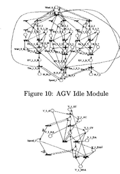
signals the AGV-Visiting Planning Module that current visiting is completed. Then, AGV proceeds t o the next visiting. Either of the communi- cation place V-lS-5-0K and V - l L 5 - 0 K is marked. It represents that sending a signal to the AGV-Calling Dispatching Module to note that loading or storing at stop 5 is completed.

AGV Idle Module

The objective of the AGV Idle Module is again to introduce a control method into the Petri-Net model

Figure 10: AGV Idle Module

Figure 11: AGV Movement Module

with an aim to guaranteeing the jam-free conditions. The method we provide is a way called recursively leav- ing strategy.

AGV Movement Module

The purpose of the AGV Movement Module is to model the characteristics of AGV's movement. For ex- ample as shown in Fig. 11, the status of AGV 1's movement can be classified into four stages, namely,

stop, accelerating , constant-speed and decelerating.

AGV Motion Planning Module

Each time when an AGV moves near from the next adjacent stop, it must be within two statuses. One is in

non-braking status, the other is in braking status. For

example, Fig. 12 illustrates the AGV Motion Planning Module, which guides an AGV to proper motion status while moving from the current stop 2. A token in the communication place V-1-Going represents that AGV 1 is in non-braking status. That the communication place V-1Braking is marked means that it is in non- braking status.

Figure 12: AGV Motion Planning Module

Figure 13: AGV Motion Control Module

Figure 14: Model relationship graph

AGV Motion Control Module

The purpose of the AGV Motion Control Module is to embed a control rule into model so that AGV can take proper motion. The basic concept of this model is described as follows. When an AGV is in non- breaking status and a t 'stop' or 'constant-speed' stage mentioned in the AGV Movement Module, a 'start ac- celerating' command will be generated. It asks AGV to accelerate. For example, Fig. 13 illustrates the AGV Motion Control Module, which generate proper motion control commands for the AGV 1. A token in the com- munication place V-LGoing represents that AGV 1 is in non-braking status. That the communication place V - l a r a k i n g is marked means that it is in non-braking status. The notations of other places and transitions are the same with those in AGV Movement Module.

4 Control Strategies and Performance Analysis by Simulation

Since the system model is large, simulation is used to obtain performance measures. In this simulation ex- periment, due to the nature of IC wafer processing, each operation time has little variation for different lots. A simulation experiment is conducted as follows. Lot Scheduling and Lot Release

Firstly, let the release rule is DETERMIN and the ar-

r .. . . .. .... . ... . . . .-

. . . I

Figure 15: The relationship between lot scheduling rule and cycle time

Figure 16: The relationship between lot release rule and number of completed lot

rival interval of input lot is 36 hours. I t means that one lot is released into the wafer factory for every 36 hours. There are three scheduling rules, FIFO, LRF(Least re- maining step firs), SSF(Shortest setup time first ), t o be implemented. Moreover, this simulation contains 10 runs. The time duration of the first run is 20000 hours and 38000 hours for the last run. The Fig. 15shows the simulation results, where SSF is better than the oth- ers do. We can see that the cycle time of lot is much long by using FIFO. Moreover, by using FIFO, the in- creasing rate of cycle time and WIP(work-in-process) is higher than the others.

We let the scheduling rule is LRF. The arrival in- terval of input lot is 36 hours for the constant input of DETERMIN(1nter-arrival times of lots are constant ) and the mean of POISS(Lots enter the facility accord-

ing t o a Poisson process ). The WIP level keeps at 600

for CONWIP( Constant work-in-process ). This simu- lation contains 10 runs. The time duration of the first run is 20000 hours and 38000 hours for the last run. In the Fig. 16, we can see that POISS having higher num- ber of completed lots than DETERMIN and CONWIP at the initial runs with shorter period of time. When the time duration of run is large, CONWIP and DE- TERMIN are better than POISS. We also can see that the number of completed lots increases fast at the ini- tial and arrives at the upper bound.

,2 ,.. ... ...

... ...

.... . . -..__.

I

Figure 17: The relationship between speed of AGV and routing rule

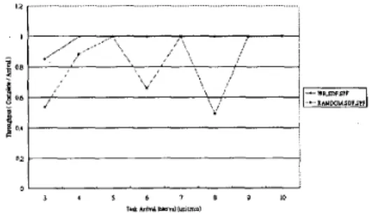
Figure 18: The relationship between visiting rule and task arrival interval

AGV Routing and AGV Visiting

In Intrabay 1, there are three multiple-load AGVs. There are three rule combinations. (WR( workload

regulating) ,SDF( shortest distance first ) ,SPF( shortest

path first )) denotes that the AGV dispatching rule

is WR, visiting rule is SDF, and routing rule is SPF. (WR,FCFS,SPF) presents that the dispatching rule is WR, visiting rule is FCFS(fist come first serve), and routing rule is SPF. (WR,FCFS,RANDOM) presents that the dispatching rule is WR, visiting rule is FCFS(fist come first serve), and routing rule is RAN- DOM. Moreover, there are five runs in this simulation. The AGV’s speed of the first run is 110.25 m/min and 1/1.75 m/min for the last run. In Fig. 17, we can see that the gap among three different combinations is increased according t o l/(speed of AGV). This phe- nomenon indicates that increasing the speed of AGV can increase performance. The Fig. 17dso show that the routing rule have more impact on performance than the visiting rule in this simulation experiment. AGV Dispatching

There are two combina-

tions,(WR,SDF,SPF),(RANDOM,SDF,SPF)tobe

im-

plemented. (WR,SDF,SPF) denotes that the AGV dis- patching rule is WR, visiting rule is SDF, and routing rule is SPF. (RANDOM,SDF,SPF) presents that the

dispatching rule is RANDOM, visiting rule is SDF, and routing rule is SPF. The loading and storing tasks are fed into the Interbay 1. The task arrival is DETER- MIN. Moreover, there are eight runs in this simulation. The task arrival interval of the first run is 3 minutes and that of the last is 10 minutes. The Fig. 18 show the results. The cycle time is increased according t o the rate of task arrival. In this simulation experiment, dispatching rule RANDOM and W R are little differ- ence in performance due t o only three AGVs. If the number of AGVs is large, we can predict that RAN- DOM and WR are much difference in performance. The Fig. 18 also shows that W R have stable perfor- mance than RANDOM.

5 CONCLUSION

The present work introduces a GSCTPN modeling of a general IC wafer fabrication system, the result net model solves the ”long” net modeling of reentrant pro- cessing problem. The validated model can be used t o answer many ”what-if’ questions, such as predicting the throughput.

REFERENCES

MengChu Zhou and Mu Der Jeng, “Modeling, Analysis, Simulation, Scheduling, and Control of Semiconductor Manufacturing System: A petri Net Approach.”, IEEE D a n . o n Semiconductor Manu- facturing, Vol. 11, pp. 333-357, 1998.

Jorn W. Janneck and Martin Naedele, “Modeling a Die Bonder with Petri Nets : A Case Study.”,

IEEE R a n . o n Semiconductor Manufacturing, Vol.

Huanxin Henry Xiong and MengChu Zhou, “Scheduling of SeMICONDUCTOR Test Facility via Petri Nets and Hybrid Heuristic Search.”, IEEE

Tran. o n Semiconductor Manufacturing, Vol. 11,

Mohamed Allam and Hassane Alla, “ Modeling and Simulation of an Electronic Component Manufac- turing System Using Hybrid Petri Nets.”, IEEE

D a n . o n Semiconductor Manufacturing, Vol. 11,

Sheng-ya Lin and Han-Pang Hung, “Modeling and Emulation of a Gurnace in IC Fab Based on Colored-Timed Petri Net.”, IEEE Tran. o n Semi-

conductor Manufacturing, Vol. 11, pp. 410-420,

1998.

Mu Der Jeng, Xiaolan Xie and Shih Wei Chou, “Modeling, Qualitative Analysis, Simulation, and Performance Evaluation of the Etching Area in an IC Wafer Fabrication System Using Petri Nets.”,

IEEE R a n . o n Semiconductor Manufacturing, Vol.

11, pp. 404-409, 1998.

pp. 384-393, 1998.

pp. 374-383, 1998.

11. PP. 358-373, 1998.