Mining High Average-Utility Itemsets
Tzung-Pei Hong
Dept. of Computer Science and Information Engineering National University of Kaohsiung
Kaohsiung, Taiwan [email protected]
Cho-Han Lee
Institute of Electrical Engineering National University of Kaohsiung
Kaohsiung, Taiwan [email protected]
Shyue-Liang Wang
Dept. of Information Management National University of KaohsiungKaohsiung, Taiwan [email protected]
Abstract—The average utility measure is adopted in this
paper to reveal a better utility effect of combining several items than the original utility measure. A mining algorithm is then proposed to efficiently find the high average-utility itemsets. It uses the summation of the maximal utility among the items in each transaction including the target itemset as the upper bounds to overestimate the actual average utilities of the itemset and processes it in two phases. As expected, the mined high average-utility itemsets in the proposed way will be fewer than the high utility itemset under the same threshold. Experiments results also show the performance of the proposed algorithm.
Keywords—utility mining, average utility, two-phase mining,
downward closure
I. INTRODUCTION
In the past, Liu et al. then presented a two-phase algorithm for fast discovering all high utility itemsets [2, 3]. In this paper, we proposed a new idea to evaluate the utilities of itemsets. Traditionally, the utility of an itemset is the summation of the utilities of the itemset in all the transactions regardless of its length. Thus, the utility of an itemset in a transaction will increase along with the increase of its length. That is, longer itemsets in a transaction result in higher utility values. Thus, using the same minimum threshold to judge itemsets with different lengths is not fair. In order to alleviate the effect of the length of itemsets and identify really good utility itemsets, the average utility measure is adopted in this paper to reveal a better utility effect of combining several items than the original utility measure. It is defined as the total utility of an itemset divided by its number of items within it. The average utility of an itemset is then compared with a threshold to decide whether it is a high average-utility itemset. An algorithm is also proposed to find all the high average-utility itemsets.
Like two-phase mining for high utility itemsets, the proposed mining algorithm for high average-utility itemsets uses average-utility upper bounds to overestimate the actual average utilities of itemsets for satisfying the downward closure property. The average-utility upper bound of an itemset is designed here as the summation of the maximal utility among the items in each transaction including the itemset. Only the combinations of the itemsets which have their average-utility upper bounds beyond the user-defined threshold are added into the candidate set in a level-wise way. The downward closure property can thus be maintained in this way. Finally, the performance of the proposed mining algorithm is verified by real-world market data.
II. REVIEW OF RELATED MINING ALGORITHMS Agrawal and Srikant proposed the Apriori algorithm [1] to mine association rules from a set of transactions. In each pass, Apriori employs the downward-closure (anti-monotone) property to prune impossible candidates, thus improving the efficiency of identifying frequent itemsets. Many other algorithms based on the property have then been proposed to discover frequent itemsets rapidly [4-7].
Traditional association-rule mining does not, however, consider the quantities sold in transactions and the profit of each item sold, which are important to some applications as well. Yao et al. thus proposed the utility model to measure how “useful” an itemset is by considering both the quantities and the profits of items [8]. In utility mining, the downward-closure property no long exists since the utility of an itemset will grow monotonically and the frequency of an itemset will reduce monotonically along with the number of items in an itemset. The two different monotonic properties make the downward-closure property invalid in utility mining. Thus, Barber and Hamilton proposed the approaches of Zero pruning (ZP) and Zero subset pruning (ZSP) to exhaustively search for all high utility itemsets in the database [9]. Li et al. then proposed the FSM, the ShFSM and the DCG methods [10, 11] to discover all high utility itemsets by taking advantage of the level-closure property. Besides, Yao proposed a framework for mining high utility itemsets based on mathematical properties of utility constraints [12]. Liu et al. then presented a two-phase algorithm for fast discovering all high utility itemsets [2, 3]. The proposed approach is based on the two-phased approach.
III. MINING HIGH AVERAGE-UTILITY ITEMSETS Traditionally, the utility of an itemset is the summation of the utilities of the itemset in all the transactions regardless of its length. Thus, the utility of an itemset in a transaction will increase along with the increase of its length. That is, longer itemsets in a transaction result in higher utility values. For example, assume a transaction is given as shown in Table 1. There are five items in the transaction, respectively denoted A to E. The value attached to each item is the quantity sold in the transaction.
TABLE 1. A TRANSACTION AS THE EXAMPLE.
TID A B C D E
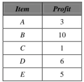
Assume the predefined profit of each item is defined in Table 2. The utility of the 1-itemset {A} in the transaction is thus calculated as 1*3, which is 3, according to the above two tables. The utility of the 2-itemset {AB} in the transaction is calculated as 1*3 + 1*10, which is 13. Similarly, the utility of the 3-itemset {ABC} is calculated as 1*3 + 1*10 + 4*1, which is 17. Accordingly, the utility of the 3-itemset {ABC} is larger than the 2-itemset {AB}, which is further larger than the 1-itemset {A}. Longer 1-itemsets result in higher utility values. This property is very obvious since longer itemsets will include some more items than their proper subsets. This effect will attenuate the judgment about whether an itemset is really better than its subsets.
TABLE 2. THE PREDEFINED PROFIT VALUES OF THE ITEMS.
Item Profit A 3 B 10 C 1 D 6 E 5
The mined itemsets in the proposed way will be fewer than those in the original way under the same threshold. Our proposed approach can thus be executed under a larger threshold than the original, thus with a more significant and relevant criterion. The approach for mining useful itemsets under the proposed criterion is stated below.
IV. THE PROPOSED ALGORITHM FOR MINING HIGH AVERAGE-UTILITY ITEMSETS
There are two phases in the proposed algorithm. In phase 1, the average-utility upper bound is used to overestimate the itemsets. In phase 2, we just need to scan the database once to check the result of phase 1 is actually high or not.
Two-Phase algorithms for mining high average-utility itemsets
INPUT:
1. A set of m items I = {i1, i2, …, ij, …, im}, each ij with a profit value pj, j = 1 to m;
2. A transaction database D = {T1, T2, …, Tn}, in which each transaction includes a subset of items with quantities; 3. The minimum average-utility threshold .
OUTPUT: A set of high average-utility itemsets.
STEP 1: Calculate the utility value ujk of each item ij in each transaction Tk as ujk = qjk*pj, where qjk is the quantity of ij in Tk for j = 1 to m and k = 1 to n.
STEP 2: Find the maximal utility value muk in each transaction
Tk as muk = max{u1k, u2k, …, umk} for k = 1 to n.
STEP 3: Calculate the average-utility upper bound ubj of each item ij as the summation of the maximal utilities of the transactions which include ij. That is:
j k j k i T ub mu
.STEP 4: Check whether the average-utility upper bound of an item ij is larger than or equal to . If ij satisfies the above condition, put it in the set of candidate average-utility 1-itemsets, C1. That is:
1 { |j j ,1 }
C i ub
j m.
STEP 5: Set r = 1, where r is used to represent the number of items in the current candidate average-utility itemsets to be processed.
STEP 6: Generate the candidate set Cr+1 from Cr with all the r-subitemsets in each candidate in Cr+1 must be contained in Cr.
STEP 7: Calculate the average-utility upper bound ubs of each candidate average-utility (r+1)-itemset as the summation of the maximal utilities of the transactions which include s. That is:
k s k s T ub mu
.STEP 8: Check whether the average-utility upper bound of each candidate (r+1)-itemsets s is larger than or equal to . If s does not satisfy the above condition, remove it from Cr+1. That is:
1 { , 1}
r s r
New C s ub
soriginal C .STEP 9: IF Cr+1 is null, do the next step; otherwise, set r = r + 1 and repeat STEPs 6 to 9.
STEP 10: For each candidate average-utility itemset s, calculate its actual average-utility value aus as follows:
| | k j jk s T i s s u au s
,where ujk is the utility value of each item ij in transaction Tk and |s| is the number of items in s. STEP 11: Check whether the actual average-utility value aus of
each candidate average-utility itemset s is larger than or equal to . If s satisfies the above condition, put it in the set of high average-utility itemsets, H. That is:
{ s , }
H s au
sC,
where C is the set of all the candidate average-utility itemsets.
V. AN EXAMPLE
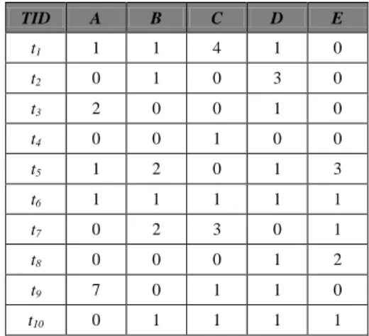
In this section, an example is given to demonstrate the proposed mining algorithm based on the average-utility of items. Assume the ten transactions shown in Table 3 are used
for mining. Each transaction consists of two features, transaction identification (TID) and items purchased.
TABLE 3. THE SET OF TEN TRANSACTION DATA FOR THIS EXAMPLE.
TID A B C D E t1 1 1 4 1 0 t2 0 1 0 3 0 t3 2 0 0 1 0 t4 0 0 1 0 0 t5 1 2 0 1 3 t6 1 1 1 1 1 t7 0 2 3 0 1 t8 0 0 0 1 2 t9 7 0 1 1 0 t10 0 1 1 1 1
Also assume that the predefined profit value for each single item is defined in Table 4.
TABLE 4. THE PREDEFINED PROFIT VALUES OF THE ITEMS.
Item Profit A 3 B 10 C 1 D 6 E 5
Moreover, the minimum average-utility threshold is set as 45.4, which is the 20% of total utility. In order to find the high average-utility itemsets from the data in Table 3, the proposed mining algorithm proceeds as follows. After STEPs 1 to 3, the upper-bound values of all the items are shown in Table 5.
TABLE 5. THE AVERAGE-UTILITY UPPER BOUNDS OF 1-ITEMSETS.
Candidate Itemset Average-Utility Upper Bound A 67 B 88 C 72 D 105 E 70
Check whether the average-utility upper bound of 1-itemsets exceeds the minimum average-utility threshold . All the items are recorded as candidate average-utility 1-itemsets,
C1, because their average-utility upper bounds are larger than or equal to the user-defined minimum average-utility threshold , which is 45.4.
Then the candidate average-utility 2-itemsets (C2) are generated from C1 and the average-utility upper bound of each
itemset is calculated. The upper-bound values of all the 2-itemsets are shown in Table 6.
TABLE 6. THE AVERAGE-UTILITY UPPER BOUNDS OF THE 2-ITEMSETS.
Candidate 2-Itemset Average-Utility Upper Bound AB 40 AC 41 AD 67 AE 30 BC 50 BD 68 BE 60 CD 51 CE 40 DE 50
After this first phase, all the candidate average-utility itemsets are shown in Table 7.
TABLE 7. ALL THE CANDIDATE AVERAGE-UTILITY ITEMSETS IN THE EXAMPLE.
Candidate Itemset Average-Utility Upper Bound A 67 B 88 C 72 D 105 E 70 AD 67 BC 50 BD 68 BE 60 CD 51 DE 50
Next, the second phase begins and the actual average-utility value aus of each candidate average-utility itemset is calculated. The actual average-utility value of each candidate average-utility itemset is then compared with the user-defined minimum average-utility threshold . In this example, the final results are shown in Table 8.
TABLE 8. HIGH AVERAGE-UTILITY ITEMSETS.
High
Average-Utility Itemset Average-Utility
B 80
D 60
Three high average-utility itemsets are generated. Note that if the traditional utility criterion is used, the results will be {B}, {D}, {AD}, {BC}, {BD}, {BE} and {DE}. The number of the high average-utility itemsets is less than that of the high utility itemset.
VI. EXPERIMENTAL RESULTS
Experiments were made to show the performance of the proposed approach. All the experiments were performed on an Intel Core 2 Duo E6550 (2.33GHz) PC with 2 GB main memory, running the Windows XP Professional operating systems. The proposed algorithm was implemented in Visual C# 9.0 and applied to a real data set.
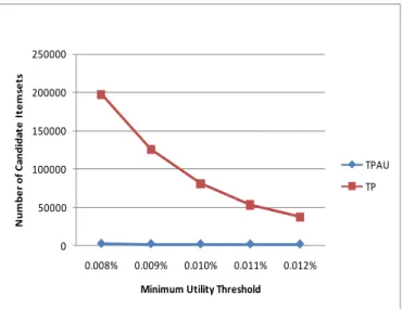
A real data set from a major grocery chain store in America was used for the experiments. There were 21,556 transactions and 1,559 distinct items in the database. Each transaction consisted of the products sold and their quantities. The average transaction length is 4.03. The total profit of the dataset is $104,450,739. Figure 1 shows the number of candidate itemsets generated by our approach (TPAU) vs. Liu’s TP. The minimum utility threshold varies from 0.008% to 0.012%. Compared to TP, TPAU generates much fewer candidate itemsets. The number of candidate itemsets generated by TPAU decreases substantially.
0 50000 100000 150000 200000 250000 0.008% 0.009% 0.010% 0.011% 0.012% N um be r of C a ndi da te I te m se ts
Minimum Utility Threshold
TPAU TP
Figure 1. Number of candidate itemsets with varying minimum utility threshold of TPAU vs. TP.
Table 9 presents the summary of the number of candidate itemsets (CI), high average-utility itemsets (HAUI), and high utility itemsets (HUI) of TPAU vs.TP. In Phase I, TPAU generates much fewer candidate itemsets. In Phase II, the number of high average-utility itemsets (HAUI) is much less than that of high utility itemsets (HUI). TPAU can discover high average-utility itemsets whose utility values are much closer to the minimum utility threshold compared to high utility itemsets.
TABLE 9. COMPARISON OF THE NUMBER OF CANDIDATE ITEMSETS (CI), HIGH AVERAGE-UTILITY ITEMSETS (HAUI), AND HIGH UTILITY ITEMSETS (HUI) OF
TPAU VS.TP.
Threshold CI (Phase I) Phase II
TPAU TP HAUI HUI
0.012% 1583 37707 1556 3497 0.011% 1614 53324 1557 4557 0.010% 1677 80735 1565 6486 0.009% 1896 125920 1579 9997 0.008% 2288 197251 1605 18005
Figure 2 shows the execution time of TPAU vs. TP. The execution time of TPAU is less than TP in all the compared minimum threshold setting.
0 500 1000 1500 2000 2500 3000 3500 0.008% 0.009% 0.010% 0.011% 0.012% Exe cut ion Ti m e (s e c. )
Minimum Utility Threshold
TPAU TP
Figure 2. Execution time with varying minimum utility threshold of TPAU vs. TP.
VII. CONCLUSIONS
This paper defines a new mining measure called average utility and proposes a two-phase mining algorithm to discover high average-utility itemsets. The proposed mining algorithm is divided into phases. In phase I, this algorithm overestimates the utility of itemsets from the perspective of transactions, this process matins the “downward closure” property to efficiently prune impossible utility itemsets level by level. In phase II, according to the candidate itemsets generated from phase I, one database scan is needed to determine the actual high average-utility itemsets. Considering that the length of itemsets is a major factor to influence the utility values of itemsets. The measure “average-utility” is used to evaluate the utility values. The experimental results show that our algorithms can obtain fewer itemsets with purer and accurate utility.
REFERENCES
[1] R. Agrawal and R. Srikant, "Fast Algorithms for Mining Association Rules in Large Databases," in Proceedings of the 20th International Conference on Very Large Data Bases: Morgan Kaufmann Publishers Inc., 1994.
[2] Y. Liu, W. Liao, and A. Choudhary, "A Two-Phase Algorithm for Fast Discovery of High Utility Itemsets," in Proceedings of the Pacific-Asia Conference on Knowledge Discovery and Data Mining (PAKDD), 2005. [3] Y. Liu, W.-k. Liao, and A. Choudhary, "A Fast High Utility Itemsets
Mining Algorithm," in Proceedings of the 1st International Workshop on Utility-based Data Mining Chicago, Illinois: ACM, 2005.
[4] M. J. Zaki, S. Parthasarathy, M. Ogihara, and W. Li, "New Algorithms for Fast Discovery of Association Rules," University of Rochester, 1997. [5] S. Brin, R. Motwani, J. D. Ullman, and S. Tsur, "Dynamic Itemset Counting and Implication Rules for Market Basket Data," in Proceedings of the 1997 ACM SIGMOD International Conference on Management of Data Tucson, Arizona, United States: ACM, 1997. [6] J. S. Park, M.-S. Chen, and P. S. Yu, "An Effective Hash-based
Algorithm for Mining Association Rules," in Proceedings of the 1995 ACM SIGMOD International Conference on Management of Data San Jose, California, United States: ACM, 1995.
[7] J. Han, J. Pei, and Y. Yin, "Mining Frequent Patterns without Candidate Generation," in Proceedings of the 2000 ACM SIGMOD International Conference on Management of Data Dallas, Texas, United States: ACM, 2000.
[8] H. Yao, H. Hamilton, and C. Butz, "A Foundational Approach to Mining Itemset Utilities from Databases," in Proc. of the 4 th SIAM International Conference on Data Mining, 2004, pp. 211-225.
[9] B. Barber and H. J. Hamilton, "Algorithms for Mining Share Frequent Itemsets Containing Infrequent Subsets," in Proceedings of the 4th European Conference on Principles of Data Mining and Knowledge Discovery: Springer-Verlag, 2000.
[10] Y. Li, J. Yeh, and C. Chang, "Efficient Algorithms for Mining Share-Frequent Itemsets," in Fuzzy Logic, Soft Computing and Computational Intelligence-11th World Congress of International Fuzzy Systems Association (IFSA 2005), 2005, pp. 534–539.
[11] Y. Li, J. Yeh, and C. Chang, "Direct Candidates Generation: A Novel Algorithm for Discovering Complete Share-Frequent Itemsets," Lecture Notes in Computer Science, vol. 3614, p. 551, 2005.
[12] H. Yao and H. J. Hamilton, "Mining Itemset Utilities from Transaction Databases," Data Knowl. Eng., vol. 59, pp. 603-626, 2006.