and t. s. liu
Department of Mechanical Engineering, National Chiao Tung University, Hsinchu 30010, Taiwan, R.O.C.
SUMMARY
Petri nets are useful for modelling a variety of asynchronous and concurrent systems, such as automated manufacturing, computer fault tolerant systems, and communication networks. This study employs an airbag inflator system as an example to demonstrate a Petri net approach to failure analysis. This paper uses Petri nets to study minimum cut sets finding, marking transfer, and dynamic behaviour of system failure. For Petri net models incorporating sensors, fault detection and higher-level fault avoidance is dealt with. Compared with fault trees that present only static logic relations between events, Petri nets indeed offer more capabilities in the scope of failure analysis. 1997 by John Wiley & Sons, Ltd. key words: Petri nets; failure analysis; reliability; airbag inflator
INTRODUCTION severity of occupants can be reduced under airbag protection8,11
when an automotive collision occurs. The fault tree analysis for detecting possible failures A failure is defined as any change in the shape,
size, or material properties of a structure, machine, of an inflator has been presented.12
In this study, the proposed fault tree will be transformed to a or component that renders it unfit to carry out its
specified function adequately.1 For the purpose of Petri net model in order to illustrate the present
failure analysis method and to show the superiority reliability assurance, failures of a system need to be
traced and analysed, especially for safety devices of Petri nets over fault trees.
The correlations between fault trees and Petri nets such as airbag systems in vehicles.
There have been many methods proposed for will be presented first in this study. Two methods for obtaining minimum cut sets then follow. The failure analysis,2 among which fault tree analysis
( FTA) is well known. It is a graphical method that third issue is the discussion of marking transfer by using a reorganized incidence matrix. Dynamic presents relationships between basic events and the
top event by logic gates and a tree construction.3 behaviour of Petri nets with failure rates formulation
will be investigated. Finally, Petri nets endowed Compared with fault trees, Petri net analysis is also
a graphical approach that performs not only the with sensors for fault detection are described. static logic relations revealed in FTA, but also
dynamic behaviour which greatly helps fault tracing
TRANSFORMATION BETWEEN FAULT TREE and failure state analysis. Moreover, the system
AND PETRI NET behaviour accounted for by Petri nets can improve
the dialogue between analysts and designers of a The basic symbols of Petri nets include:13
s : Place, drawn as a circle, denotes event system.4
Nowadays, deaths and injuries resulting from the 3 : Transition, drawn as a bar, denotes event transfer
use of motor vehicles are at a terribly high level
worldwide. Available statistics report that over ↑ : Arc, drawn as an arrow, between places and transitions
154,000 deaths and 5,000,000 injuries occur each year all over the world.5
As a result, airbag systems d : Token, drawn as a dot, contained in places, denotes the data.
used for passengers’ protection are fitted on modern vehicles in rapidly increasing numbers.6–12
An airbag The transition is said to fire if input places satisfy an enabled condition. Transition firing will remove system is also called a supplemental inflatable
restraint8 or supplemental restraint system9 and is one token from all of its input places and put one
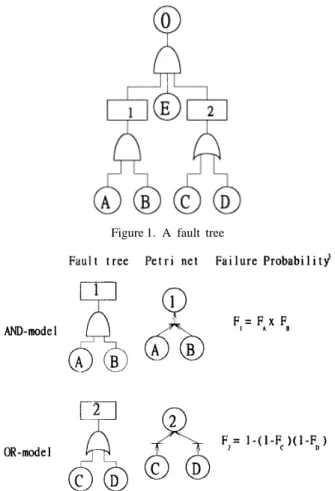
token into all of its output places.14 Figure 1 is a
composed of three major subsystems: inflator and
bag assembly, diagnostic module, and crash sen- fault tree example in which events A, B, C, D, and E are basic causes of event 0. The logic relations sors.10 The inflator and bag assembly is used to
inflate an airbag so that the head and chest injury between the events are described as well. The
corre-CCC 0748–8017/97/030139–13 $17.50 Received 30 December 1996
2. If the output place is connected by one arc from a transition then the numbers of the input places should be put down in a column. This accounts for AND-models.
3. The common entry located in rows is the entry shared by each row.
Figure 1. A fault tree
4. Starting from the top event down to the basic events until all places are replaced by basic events, a matrix is thus formed, called the basic event matrix. The column vectors of the matrix constitute cut sets.
5. Remove the supersets from the basic event matrix and the remaining column vectors become minimum cut sets.
This top-down fashion facilitates obtaining minimum cut sets logically. The differences between the present method and the MOCUS19
algorithm include:
1. The present method is based on Petri net mod-els, whereas the MOCUS algorithm is based
Figure 2. Correlations between fault tree and Petri net
on fault trees.
2. Events in fault trees correspond to places in lations between fault tree and Petri net are shown
Petri nets. Using Petri nets, logic gates do not in Figure 2. Figure 3 is the Petri net transformed
appear in the matrix, in which only places are from Figure 1.
dealt with, whereas by MOCUS all logic gates One potential problem in the deployment of an
in addition to events are processed in the automobile airbag is an inadequate inflator system
generating steps. output that may be caused by delayed output,
3. The structure of the matrix looks like that of reduced output or no output, for which an inadequate
the Petri net itself such that it is amenable to inflator output in airbags has been investigated.12
constructing the matrix; however, tables com-Figure 4 shows its proposed fault tree. As an
illus-posed of generating steps using MOCUS look trating example, based on the above statement, it can
unlike structures of fault trees. be tranformed into Petri net as shown in Figure 5.
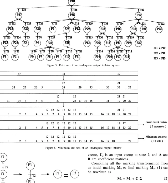
Its sequence numbers of places and transitions are
Figure 6 illustrates minimum cut sets used to search prescribed, starting from basic events to the top
the inadequate output for an inflator system, depicted event from the left side to the right side in the
in Figure 4, by the matrix method. Petri net.
Minimum cut sets can be derived in an opposite direction, i.e. from basic places to the top place. MINIMUM CUT SETS Transitions with T=0 are called immediate
tran-sitions.14
If a Petri net has immediate transitions, There have been quite a few methods used to
gener-i.e. the token transfer between places does not take ate minimum cut sets for fault trees.15–18
By contrast,
time, then it can be abosrbed to a simplified form a matrix method2 for finding minimum cut sets
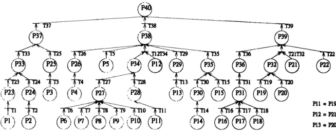
called the equivalent Petri net. Figure 7 shows the principle of absorption, by which Figure 8 is the equivalent Petri net resulting from Figure 5. After absorption, all the remaining places are basic events. The equivalent Petri net exactly constitutes the mini-mum cut sets, i.e. the input of each transition rep-resents a minimum cut set. This method is in bot-tom-up fashion.
Therefore, both top-down and bottom-up methods have been proposed in this work to find minimum
Figure 4. Fault tree analysis—inadequate system output
Figure 5. Petri net of an inadequate output inflator system
Figure 6. Minimum cut sets of an inadequate output inflator
vector, Uk is an input vector at state k, and A and
B are coefficient matrices.
Combining all the marking transformation from an initial marking M0 to final marking Mn, (1) can
be rewritten as
Mn=M0+C S (2)
or
Mn−M0=C S (3)
where C is an m×n matrix called the incidence
Figure 7. The absorption principle of equivalent Petri nets
matrix, m and n being the total numbers of places MARKING TRANSFER and transitions, respectively. In addition, entries of
C are A marking of a Petri net is defined as the total
number of tokens at each place,20 denoted by a
cij=1, if transition j has an outgoing
column vector M. Thus the vector Mk=(n1, n2, . . ., arc to place i
nm)Trepresents that token numbers of places P1, P2, cij= −1, if transition j has an incoming
. . ., Pm at state k are n1, n2, . . ., nm, respectively. arc from place i
Consequently, Petri nets can be expressed in state c
ij=0, if there is no arc between them
space form, which gives the next state Mk+1 from
Moreover, cij=1 (−1) means place i gains (loses)
its previous state Mk:13
one token if transition j fired. In (3), S denotes a Mk+1=A Mk+B Uk, k=1,2,. . . ( 1) column vector, called the firing-count vector,13
whose entry i denotes the number of times that where Mkis the marking at state k, an m×1 column
Figure 8. Equivalent Petri net of Figure 5
transition i fires in a firing sequence such that M0 Since the sequence numbers of places and
tran-sitions are the same, Ti may fire when Pi holds
is transformed into Mn.
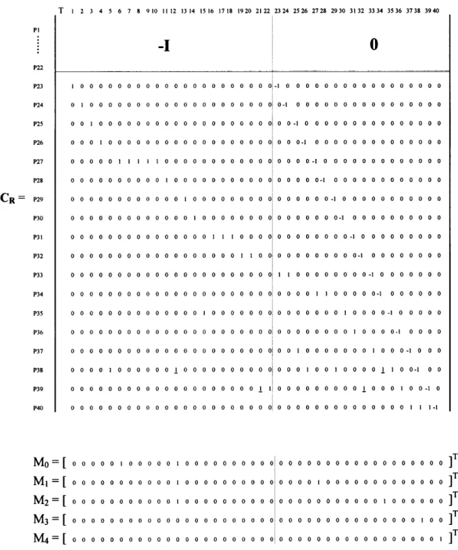
To renumber transitions, a method2 is employed tokens. Suppose the initial marking for the
inad-equate output inflator (Figure 9) is to establish a reorganized incidence matrix CR that
provides marking transfer steps from M0 up to Mn.
M0=[0000010000010000000000000000000000000000 ] T
The rules for transition renumbering are:
i.e. each of P6 and P12 possesses a token, which
1. Let the number assigned to each transition be
from Figures 4 and 5 represent ball weld rupture the same number of the input place in this
and failure of the low pressure sensor (LPS) switch transition, no matter whether the input is
mul-in the airbag mul-inflator. Smul-ince P6 holds a token, T6
tiple or not.
fires. Note that in the T6 column in CR, only the
2. If the transition has multiple inputs, then the
entry CR27,6=1, which means that P27 gains a token
number of this transition includes every input
when T6 fires. Consequently, a token moves from
number.
P6 to P27. However, T12will not fire, since the entry
CR38,12 is underlined, which means it cannot fire
As a result, the renumbered Petri net for Figure 5
is shown in Figure 9. unless both P12 and P34 hold tokens at the same
time. Thus, the marking becomes The rules for constructing the reorganized
inci-dence matrix are:
M1=[0000000000010000000000000010000000000000 ]T
1. Assign each entry of the incidence matrix CR
In a similar manner, CR34,27=1, as shown in
in a manner similar to C as described
pre-Figure 10, and T27 fires such that the token moves
viously, but append one column to CR.
Accord-from P27 to P34. Therefore,
ingly, it becomes an m×m square matrix
where m is the total number of places. Besides, M2=[0000000000010000000000000000000001000000 ]T
let entry CRm,m be −1.
Since CR38,12 = CR38,34=1 according to Figure 10
2. Underline all the entries that consititute
mul-and both P12 and P34 hold a token, T12T34 fires so
tiple incoming transitions.
as to provide P38 a token. Accordingly,
Once the reorganized incidence matrix is done, the
M3=[0000000000000000000000000000000000000100 ]T
upper-left q×q elements form a negative identity
square matrix and there is a q×( m−q) null matrix Note that CR40,38=1 and T38 fires. A token hence
moves to P40, i.e. the top event of this airbag inflator
at the upper-right, where q is the total number of
basic places. The incidence matrix CRresulting from system occurs, with marking
Figure 9 is shown in Figure 10, where q is 22,
M4=[0000000000000000000000000000000000000001 ]T
m is 40 and CR38,12, CR38,34, CR39,21 and CR39,32
are underlined. The associated reorganized incidence matrix CR and
Figure 10. Marking transfer steps M0up to M4 observed from the reorganized incidence matrix CR
the marking transfer steps based on the reorganized behaviour of system failure is defined as the system failure state with time varied, and is determined by incidence matrix are illustrated in Figure 10. This
method enables deriving marking transfer by direct the movement of tokens in a Petri net model. A merit of the approach is that the dynamic behaviour observation without calculation, which is different
from (2) and ( 3) that were proposed by Hura and of a system failure can be investigated by Petri nets,20 whereas it cannot be done by fault trees.
Atwood.13 Failure state evolution can be observed,
as illustrated in the inflator example. This is one of Define mi(t) as the marking of Pi, i.e. the token
quantity at time t for place i, and assume that a the advantages for failure analysis of using the Petri
net approach. basic place generates a token at every time period
of T, i.e. the time between failures is T. Accordingly, the timed marking of Pi performs like a stair
func-DYNAMIC BEHAVIOUR
tion. It is equal to zero during the first period, one Since the vector Mk represents the marking in a during the second period, two during the third
per-Petri net at state k, the failure state of a system iod, etc. Hence, a timed marking for a place can may vary with time. Hence, the markings of a be written as21
Figure 13. Single level transition with multi-inputs for the OR-model
Figure 11. Single transition with single input
=
O
` k=1 u(t−kT−d1−d2−. . .−dtop) =O
` k=1 u(t−kT−D) (7) where D =O
top s=1ds denotes the total delay time due
to transitions.
2. Transition with multi-inputs
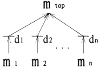
(A) OR-model. According to the property of Petri nets,21
the output marking of an OR-model is the summation of input markings with delay times; i.e.
mtop(t)=[ m1(t)d1+m2(t)d2+. . . mn(t)dn] (8) Figure 12. Hierarchial transition with single input
(a) Single level transition (Figure 13) + 2[u(t−2T)−u(t−3T)] + . . .=u(t−T)
From (4), let basic place markings be + u(t−2T) + u(t−3T) + . . . ( 4) m1(t)=
O
` k=1 u(t−kr1T) =O
` k=1 u(t−kT)where u(t) is a unit step function. m
2(t)=
O
`k=1
u(t−kr2T)
The timed marking transfer of places can be described as follows:
. . .
1. Transition with single input m
n(t)=
O
`
k=1
u(t−krnT) (9)
In this case, the marking for an output place is
where r1 to rn denote factors to account for different
the input marking with delay time d involved.
periods among events. Hence riT, i=1,2,3,. . .,n,
represent the token generation period at place Pi.
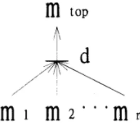
(A) Single transition (Figure 11). According to
Substituting (9) into (8) yields the top place marking ( 4), let mtop(t) =
O
` k=1 u(t−kr1T−d1) +O
` k=1 u(t−kr2T−d2) m1(t)=O
` k=1 u(t−kT) ( 5) Hence, + . . . +O
` k=1 u(t−krnT−dn) ( 10) m2(t) =m1(t)d=O
` k=1 u(t−kT−d ) ( 6) =O
n s=1 [O
` k=1 u(t−krsT−ds) ]where d denotes the delay time due to transition. (B) Hierarchial transition (Figure 12). The
(b) Hierarchical transition (Figure 14 ) marking of the top place in this construction is
derived as From (8) and in accordance with Figure 14,
mtop( t)=[. . .({[m1(t)d1+ m2(t)d2]d3+ m4(t)d4}d5
Figure 15. Single transition with multi-inputs for the AND-model
(B) AND-model. The output marking of an AND-model is the minimal number among input markings21 with time delay; i.e.
mtop(t)=min [m1(t)d, m2( t)d, . . . . mn( t)d]
( 12) (a) Single transition (Figure 15 )
From (9) and (12 ), the top place marking of
Figure 14. Hierarchical transition with multi-inputs for the
OR-Figure 15 is model mtop(t) =min[
O
` k=1 u(t−kr1T−d),+ m6(t)d6)d7+. . .+ mtop-3(t)dtop-3]dtop-2 + mtop-1(t)dtop-1
O
` k=1 u(t−kr2T−d), . . .,O
` k=1 u(t−krnT−d)] =[. . .({[O
` k=1 u(t−kr1T−d1) +O
` k=1 u(t−kr2T−d2)]d3 =min [O
` k=1 u(t−kriT−d)], (i=1,2,3,. . .,n) ( 13) +O
` k=1 u(t−kr4T−d4)}d5+O
` k=1 u(t−kr6T−d6))d7 =O
` k=1 u(t−krbT−d) +. . .+O
` k=1u(t−krtop-3T−dtop-3)]dtop-2
where rb is the largest number of all ri. In other
words, the token generation period of Pb is the
+
O
`
k=1
u(t−krtop-1T−dtop-1)
longest one among all input places. (b) Hierarchical transition (Figure 16) =
O
`k=1
u(t−kr1T−d1−d3−d5−. . .−dtop-2)
From (12) and Figure 16, the top place marking of this construction is expressed by
+
O
` k=1 u(t−kr2T−d2−d3−d5−. . .−dtop-2) +O
` k=1 u(t−kr4T−d4−d5−d7−. . .−dtop-2) +O
` k=1 u(t−kr6T−d6−d7−d9−. . .dtop-2) +. . .+O
` k=1u(t−krtop-3T−dtop-3−dtop-2)
+
O
`
k=1
u(t−krtop-1T−dtop-1)=
O
` k=1 u(t−kr1T−O
R s=1 d2s−1)(11 ) +O
R−1 s=1 [O
` k=1 u(t−kr2sT−d2s−O
R−1 u=s d2u+1)] +O
` k=1u(t−krtop-1T−dtop-1)
Figure 16. Hierarchical transition with multi-inputs for the AND-model
23 24 33
+ m3(t)d3,d25=[m1(t)d1,d23
+ m2(t)d2,d24]d33+ m3( t)d3,d25
Finally, employing (7) that deals with delay time at transitions leads to m37(t) =m1(t)d1,d23,d33+ m2( t)d2,d24,d33+ m3(t)d3,d25 ( 15) In a similar fashion, m38(t)=m26(t)d26+ m5(t)d5+ min [m34(t)d34, m12(t)d12] + m29(t)d29+ m35(t)d35 =m4(t)d4,d26+ m5(t)d5+ min ({[ m6(t)d6,d27,d34 + m7( t)d7,d27,d34+ m8(t)d8,d27,d34 + m9(t)d9,d27,d34+ m10(t)d10,d27,d34] ( 16) + [m11(t)d11,d28,d34]},m12(t)d12) Figure 17. Fault detection arrangement
+ m13(t)d13,d29+ m14(t)d14,d30,d35+ m15(t)d15,d35
mtop(t)=min ([. . .min {[min ({min Besides,
[ m1(t)d1, m2( t)d1]}d2, m4(t)d2)]d3, m39(t) =m36(t)d 36+ min [m32(t)d32, m21( t)d21] m6(t)d3}d4. . .]dR, mtop-1(t)dR) + m22(t)d 22=m16(t)d16,d31,d36+ m17( t)d17,d31,d36 + m18(t)d18,d31,d36+ min {[m19(t)d19,d32 ( 17) =min [
O
` k=1 u(t−kr1T−d1−d2−. . .−dR), + m20(t)d20,d32], [m21(t)d21]} + m22(t)d22As a consequence, the marking of the top place is
O
` k=1 u(t−kr2T−d1−d2−. . .−dR), written as m40(t)=m37(t)d37+ m38(t)d38+ m39(t)d39O
` k=1 u(t−kr4T−d2−d3−. . .−dR), =O
` k=1 u(t−kr1T−d1−d23−d33−d37)O
` k=1 u(t−kr6T−d3−d4−. . .−dR), +O
` k=1 u(t−kr2T−d2−d24−d33−d37)O
` k=1 u(t−kr8T−d4−d5−. . .−dR), . . ., +O
` k=1 u(t−kr3T−d3−d25−d37)O
` k=1 u(t−krtop-1T−dR)] (14) +O
` k=1 u(t−kr4T−d4−d26−d38) =min [O
` k=1 u(t−kr1T−O
R s=1 ds), +O
` k=1 u(t−kr5T−d5−d38)O
` k=1 u(t−kr2T−O
R s=1 ds), + min ({O
10 s=6 [O
` k=1 u(t−krsT−ds−d27−d34−d38)]O
` k=1 u(t−kr2vT−O
R s=v ds)], (v =2,3,4,. . .,R) +O
` k=1 u(t−kr11T−d11−d28−d34−d38)},Based on (4) to ( 14), the marking transfer for
inadequate system output of the inflator, as depicted
O
`k=1
u(t−kr12T−d12d38))
Figure 18. Token transfer in different situations
Moreover, the failure rate22 F(t) of this system can
be written as +
O
` k=1 u(t−kr13T−d13−d29−d38) F(t) =m40(t)/t ( 19)Failure rates derivation using the marking transfer +
O
`
k=1
u(t−kr14T−d14−d30−d35−d38)
calculation has been illustrated. Since the dynamic behaviour of a system failure can be investigated by Petri nets,20 whereas it cannot be done by fault
+
O
`k=1
u(t−kr15T−d15−d35−d38) (18 )
trees, it is also one of the advantages for failure analysis gained from the Petri net approach over FTA. +
O
18 s=16 [O
` k=1 u(t−krsT−ds−d31−d36−d39)]FAULT DETECTION AND REPAIR RATE + min {
O
20 s=19 [O
` k=1 u(t−krsT−ds−d32−d39)],Once a token appears in a place of a Petri net, it represents that failure occurs in the system. If failure can be detected by sensors and properly processed
O
`k=1
u(t−kr21T−d21−d39)}
in the early stage, the undesired and more serious faults of the system can be avoided. Therefore, sensors play an important role in fault detection. By +
O
`
k=1
u(t−kr22T−d22−d39)
Figure 19. Fault detection arrangement for an inadequate output inflator system
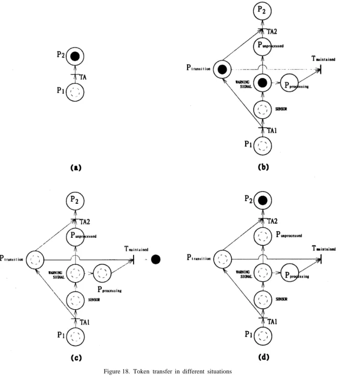
higher-level faults by incorporating sensors into a ment, with a concept of conditional transition as
shown in Figure 17, which is endowed with sensors Petri net has been described in this study. All the above methods have been applied to an airbag to achieve fault detection and higher-level fault
avoidance. In this arrangement, Ptransition represents inflator system, with inadequate output as the top
event. a transitional state inserted between P1 and P2,
which is the original path from P1 to P2 without The transformation between fault trees and Petri
nets is always achievable. However, in contrast to sensors installed, and its duration is T1 plus T2.
Figure 18(a) shows a Petri net where if P1 holds a fault trees that only present static logic relations
between events, the Petri net approach not only token, i.e. P1 failure occurs, P2 will take place
through the transition TA which represents the tran- contains the capability of FTA, but also facilitates direct observation of marking transfer, analysing sitional time between P1 and P2 failures. However,
in the fault detection arrangement depicted in dynamic behaviour of system failure, fault detection arrangements, and repair rate calculations for failure Figure 18(b), P1 failure fires TA1 to put a token
into a transitional place that represents the tran- analysis. It is worth constructing Petri net models rather than establishing fault trees at the outset of sitional state. In addition, a token is put into the
detection sensor that enables the warning signal, i.e. system failure analysis in order to gain the above-mentioned advantages.
P1 fault is detected. As soon as a processing action
is taken, the token in the processing place that comes from the detection sensor together with the
REFERENCES token in the transitional place will leave the Petri
net through a transition that accounts for mainte- 1. B. S. Dhillon, Mechanical Reliability: Theory, Models and
Applications, AIAA Education Series, Washington DC, 1988. nance, such that a higher-level fault, i.e. P2 failure, 2. S. B. Chiou, ‘Failure analysis in reliability engineering using
is avoided, as depicted in Figure 18(c). By contrast, Petri nets’, MS Thesis, National Chiao Tung University,
Taiwan, Republic of China, 1995.
if the warning signal is ignored, as shown in
3. Patrick D. T. O’Connor, David Newton and Richard Bromley,
Figure 18(d), the token in the detection sensor, after
Practical Reliability Engineering, Wiley, Chichester,
moving to the unprocessed place, together with the England, 1995.
4. J.-F. Ereau and M. Saleman, ‘Modeling and simulation of a
token in the transitional place will enable transition
satellite constellation based on Petri nets’, Proceedings of
TA2 to fire. Consequently, P2 failure occurs. the Annual Reliability and Maintainability Symposium, IEEE,
Petri net models enable designers to determine 1996, pp. 66–72.
5. H. W. Mathews, Jr. ‘Global outlook of safety and security
where sensors should be installed in order to obtain
systems in passenger cars and light trucks’, Proceedings of
warning signals from adequate places. Figuire 19
the International Congress on Transportation Electronics, shows the Petri net for an inadequate output in an Vehicle Electronics, Meeting Society’s Needs: Energy,
Environment, Safety, Dearborn, 1992, pp. 71–93. inflator system with fault detection sensors. The
6. M. Ostertag, E. Nock and U. Kiencke, ‘Optimization of
fault detection arrangement can be installed at any,
airbag release algorithms using evolutionary strategies’,
Pro-or all if necessary, locations between basic places ceedings of the 4th IEEE Conference on Control Applications,
1995, pp. 275– 280.
and the top place. The failure rates of P37, P38, and
7. T. D. Hendrix, J. P. Kelley and W. L. Piper, ‘Mechanical
P39 depend on m37(t), m38( t), and m39( t), depicted
versus accelerometer based sensing for supplemental
inflat-in (15), ( 16), and (17 ), respectively, i.e. able restraint systems’, Proceedings of the International Con-gress on Transportation Electronics, Vehicle Electronics,
F37(t)=m37(t)/t Meeting Society’s Needs: Energy, Environment, Safety, 1990, pp. 13–22.
F38(t)=m38(t)/t 8. D. Bergfried, W. Nitschke and M. Rutz. ‘Airbag control modules—performance and reliability’, Proceedings of the
F39(t)=m39(t)/t (20)
International Congress on Transportation Electronics, Vehicle Electronics, Meeting Society’s Needs: Energy, If repair rates of P37, P38, and P39 are greater than
Environment, Safety, Dearborn, 1992, pp. 155–162.
F37(t), F38(t), and F39( t), respectively, the top place 9. K. H. Yang, B. K. Latouf and A. I. King, ‘Computer simulation of occupant neck response to airbag deployment
P40 will never happen.
in frontal impacts’, Journal of Biomechanical Engineering, 114, (3 ), 327–331 (1992 ).
10. S. Goch, T. Krause and A. Gillespie, ‘Inflatable restraint
CONCLUSIONS system design considerations’, Proceedings of the Inter-national Congress on Transportation Electronics, Vehicle This paper has presented failure analysis for an Electronics, Meeting Society’s Needs: Energy, Environment,
Safety, 1990, p. 23–43. airbag inflator system by using Petri nets. Once the
11. S. M. Mahmud and A. I. Alrabady, ‘A new decision making
Petri net dealing with system failure is established,
algorithm for airbag control’, IEEE Transactions on Vehicular
the associated minimum cut sets can be constructed Technology, 44, (3 ), 690–697 (1995 ).
12. Sheng-Hsien Teng and Shin-Yann Ho, ‘Reliability analysis
15. K. Dimitri, Reliability Engineering Handbook, Vol. 2, Pren- Laboratory, Chong Shan Institute of Science and
Tech-tice-Hall, Englewood Cliffs, New Jersey, 1991. nology, Taiwan. Since 1991, he has been an instructor in 16. J. B. Fussell and W. E. Vesely, ‘A new methodology for the Department of Mechanical Engineering at Chin Yi obtaining cut sets for fault trees’, Transactions of American Institute of Technology, Taiwan. Since 1994 he has been
Nuclear Society, 15, 262–263 (1972 ).
a Ph.D. student majoring in Mechanical Engineering at
17. L. Rosenberg, ‘Algorithm for finding minimal cut sets in a
National Chiao Tung University, Taiwan. His research
fault tree’, Reliability Engineering and System Safety, 53,
interests are in reliability, data acquisition and automatic
67– 71 (1996 ).
control.
18. J. D. Andrews and T. R. Moss, Reliability and Risk
Assess-ment, Longmans, 1993.
19. J. B. Fussell, E. B. Henry and N. H. Marshall, ‘Mocus—a T. S. Liu received the BS from National Taiwan Univer-computer program to obtain minimal cut sets from faulty sity in 1979 and the MS and Ph.D. from the University
tree’, ANCR-1156, 1974. of Iowa, U.S.A. in 1982 and 1986, respectively, all in
20. M. Malhotra and K. S. Trivedi, ‘Dependability modeling
mechanical engineering. Since 1987, he has been with
using Petri-nets’, IEEE Transactions on Reliability, 44, (3),
National Chiao Tung University, Taiwan where he is
428–440 (1995 ).
currently Professor. From 1991 to 1992 he was a visiting
21. J. L. Peterson, Petri Net Theory and the Modeling of Systems,
researcher in the Institute of Precision Engineering, Tokyo
Prentice-Hall, Englewood Cliffs, New Jersey, 1981.
Institute of Technology, Japan. His current research
inter-22. K. C. Kapur and L. R. Lamberson, Reliability in Engineering