運用泛型演算法解決多頻道無線網狀網路上頻道配置與繞徑問題

全文

(1)!. ୮ Ҥ ҫ ೮ δ Ꮱ! !. !. !. !. !. 資訊科學與工程研究所碩士論文. 運用泛用型演算法解決多頻道無線網狀網路上頻道配置與繞徑問題 Channel Assignment and Routing for Multi-Channel Wireless Mesh Networks Using Generic Algorithms. 研究生：劉上群指導教授：陳. 健教授. 中華民國. 九十四. 年十月.

(2) 運用泛型演算法解決多頻道無線網狀網路上頻道配置與繞徑問題 Channel Assignment and Routing for Multi-Channel Wireless Mesh Networks Using Generic Algorithms. 研究生：劉上群. Student：Shang-Chun Liu. 指導教授：陳. Advisor：Chien Chen. 健. 國立交通大學資訊科學與工程研究所碩士論文. A Thesis Submitted to Institute of Computer Science and Engineering College of Computer Science National Chiao Tung University in partial Fulfillment of the Requirements for the Degree of Master in Computer Science October 2005 Hsinchu, Taiwan, Republic of China. 中華民國九十四年十月.

(3) 運用泛型演算法解決多頻道無線網狀網路上頻道配置與繞徑問題. 研究生 : 劉上群. 指導教授: 陳. 健. 國立交通大學資訊科學與工程系. 中文摘要. 近年來，無線網狀網路的應用，對於最後一哩(last-mile)寬頻網際網路存取服務，提供了相當大的原動力。儘管實體層技術不斷的進步，干擾依舊是限制傳統單頻道無線網路頻寬的主要因素。因此，利用多個不重疊頻道與多無線網路介面卡，干擾可有效的降低，無線網路頻寬便能大幅的增加。本篇文章首先提出一個探索式頻道配置與繞徑演算法(LASRR)，用來解決單一流量需求的繞徑問題，並配置頻道於未配置的連線上。基於 LASRR 演算法，針對不同的流量需求，我們進一步發展出兩種以泛型為基礎的演算法：以攀爬式(Hill-Climbing)為基礎的繞徑與頻道配置演算法 (HCRCA) ，用於靜態流量需求；以模擬退火 (Simulated-Annealing)為基礎的繞徑與頻道配置演算法(SARCA)，用於動態流量需求。前者簡明地利用多次重複執行的動作，以達到最大網路傳輸量的目標，後者亦利用預先定義的評估函式，針對各別來到的需求，能有效降低阻塞的機率。最後，經由實際的模擬並且比較現有的演算法，驗證整體效能的增進。. 關鍵字：無線網狀網路、探索式頻道配置與繞徑、泛型演算法、攀爬式演算法、模擬退火演算法。 i.

(4) Channel Assignment and Routing for Multi-Channel Wireless Mesh Networks Using Generic Algorithms. Student: Shang-Chun Liu. Advisor: Dr. Chien Chen. Institute of Computer Science and Engineering National Chiao Tung University. Abstract In recent years, the application of wireless mesh network has provided a quite attractive solution for last-mile broadband internet access service. Despite the unceasing advance in wireless physical-layer technologies, interference is still the major factor that limits the bandwidth in conventional single-channel wireless networks. Therefore, by exploiting multiple non-overlap channels and multiple NICs environment, interference can be decreased and the available bandwidth can be increased substantially. In this study, a heuristic routing and channel assignment algorithm, called Load aware Single Request Routing algorithm (LASRR) is first proposed to route a single traffic request and assigns channels to the links on the route that have not been assigned yet. Base on LASRR, we further develop two generic based algorithms that aim at different traffic requirements; Hill-Climbing based Routing and Channel Assignment algorithm (HCRCA) for static traffic requirement and Simulated-Annealing based Routing and Channel Assignment algorithm (SARCA) for dynamic traffic requirement. While the former simply commits several iterations to maximize the network throughput, the later also utilizes a pre-defined cost ii.

(5) functions to minimize the blocking probability for each coming request. Finally, simulation is conducted to demonstrate the performance improvement compared to an existing algorithm.. Keywords: Wireless mesh networks (WMNs); heuristic routing and channel assignment; generic algorithm; Hill-Climbing (HC); Simulated-Annealing (SA).. iii.

(6) 誌謝本篇論文的完成，我要感謝這兩年來給予我協助與勉勵的人。首先要感謝我的指導教授陳健博士，即使這段期間遭遇了不少的挫折，陳老師對我的指導與教誨使我都能在遇到困難時另尋突破，在研究上處處碰壁時指引明路讓我得以順利完成本篇論文，在此表達最誠摯的感謝。同時也感謝我的論文口試委員，交大的簡榮宏教授、陳穎平教授及海大的馬永昌教授，他們提出了許多的寶貴意見，讓我受益良多。. 感謝與我一同努力的學長陳盈羽，由於我們不斷互相討論及在論文上的協助，使我能突破瓶頸，研究也更為完善。另外我也要感謝實驗室的同學、學弟們，王獻綱、徐勤凱、陳咨翰、高游宸、周家聖、郭修嘉、江長傑、田濱華、陳健凱以及莊順宇等人，感謝他們陪我度過這兩年辛苦的研究生活，在我需要協助時總是不吝伸出援手，陪我度過最煩躁與不順遂的日子。. 特別感謝我的朋友，吳佩芷、陳映方、蘇智宏及許多大學時代的好友們，他們在精神上給我莫大的鼓勵，傾聽我內心的聲音並帶給我無比的溫暖，指導我做出了許多正確的抉擇，而不致迷失了自我。這些好朋友們就像是明燈般照亮了昏暗的旅程，並陪伴我度過枯燥的研究生涯。. 最後，我要感謝家人對我的關懷及支持，他們含辛茹苦的栽培，使我得以無後顧之憂的專心於研究所課業與研究，我要向他們致上最高的感謝。. iv.

(7) Table of Content 中文摘要 ........................................................................................................................i Abstract.........................................................................................................................ii 誌謝...............................................................................................................................iv Table of Content ...........................................................................................................v List of Figures..............................................................................................................vi Chapter 1: Introduction ..............................................................................................1 Chapter 2: Related work .............................................................................................6 2.1 Interference Model and Capacity for WMNs ..................................................6 2.2 Channel Assignment Strategies for Multi-Channel WMNs.............................8 2.2.1 Single Network Interface Card .............................................................8 2.2.2 Multiple Network Interface Card..........................................................9 2.3 Hill Climbing and Simulated Annealing........................................................11 2.3.1 Hill Climbing ......................................................................................11 2.3.2 Simulated Annealing...........................................................................12 Chapter 3: Proposed Routing and Channel Assignment Algorithms....................14 3.1 The Variables and Objective Function ...........................................................14 3.2 Load Aware Single Request Routing Algorithm............................................15 3.3 Hill Climbing Based Routing and Channel Assignment................................17 3.4 Simulated Annealing Based Routing and Channel Assignment ....................19 Chapter 4: Simulation Results..................................................................................27 4.1 Simulation Result of HCRCA – Static Traffic ...............................................28 4.2 Simulation Result of SARCA – Dynamic Traffic..........................................32 Chapter 5: Conclusions .............................................................................................38 Reference: ...................................................................................................................39. v.

(8) List of Figures Fig. 1. An example of wireless mesh network. ..............................................................2 Fig. 2. When node F is transmitting to node G (edge F-G is active). None of edge in this figure can be operate simultaneously, for k = 2. .....................................................3 Fig. 3(a). An illustration of static traffic requirement. ...................................................4 Fig. 3(b). An illustration of dynamic traffic requirement. .............................................4 Fig. 4. Collision domain of active link. .........................................................................7 Fig. 5. Classification of channel assignment strategies. ................................................8 Fig. 6. Identical and non-identical channel assignment...............................................10 Fig. 7(a). HC iteration at each time for the best solution.............................................12 Fig. 7(b). SA allowing cost uphill moves up at each time t for global optima. ...........13 Fig. 8(a). Formal procedure of Hill Climbing..............................................................13 Fig. 8(b). Formal procedure of Simulated Annealing. .................................................13 Fig. 9. Available capacity on link (4, 5) is Max{C – (a + b + c + e + f + g), 0}. If all links are using the same channel..................................................................................15 Fig. 10(a). Load aware single request routing algorithm (LASRR). ...........................17 Fig. 10(b). Criterion of non-conform links (if NIC=2 for all nodes). Italic number represents the channel already assigned on the link; Bold represents the available channel on link (a, b). ..................................................................................................17 Fig. 11. Hill climbing based routing and channel assignment algorithm. ...................19 Fig. 12. Ripple-effect of channel change (NIC = 2). ...................................................23 Fig. 13. Neighborhood structure: a capacity release algorithm ...................................24 Fig. 14. Examples of capacity release algorithm. ........................................................25 Fig. 15. A 10x10 grid topology with 100 nodes...........................................................27 Fig. 16. The overall network throughput with 2 NICs per node..................................29 Fig. 17. The overall network throughput with 3 NICs per node..................................30 Fig. 18. The overall network throughput with 4 NICs per node..................................30 Fig. 19. The average network overall throughput with 2-3-4 NICs per node..............31 Fig. 20. Impact of different traffic request pairs and number of NICs on overall throughput improvements. ...........................................................................................31 Fig. 21. The overall network blocking probability with 2 NICs per node...................33 Fig. 22. The overall network blocking probability with 3 NICs per node...................34 Fig. 23. The overall network blocking probability with 4 NICs per node...................34 Fig. 24. The network throughput curve with 2 NICs per node. ...................................35 Fig. 25. The network throughput curve with 3 NICs per node. ...................................36 Fig. 26. The network throughput curve with 4 NICs per node. ...................................37. vi.

(9) Chapter 1: Introduction For several years, wireless hardware has been widely used in local area networks and is becoming more and more popular because of its decreasing cost compared with the wired networks. Although designing multi-hops wireless networks has been an active topic of research for many years, the available bandwidth is still limited due to the interference from adjacent nodes. Fortunately, IEEE 802.11a/b/g and 802.16 standards allow multiple non-overlapping (or orthogonal) channels to be used simultaneously to increase the aggregate bandwidth available to the users. For example, 802.11b offers 3 non-overlapping channels, while 12 for 802.11a. Consequently, providing each node with multiple radios (NICs) and assign them to different channels can exploit the advantage of multiple channel property, and may offer a promising avenue for improving the capacity of networks.. Recently, wireless Mesh networks (WMNs) are being deployed as a solution to extending the reach of the last-mile access to the wired internet, using a multi-hop configuration, as shown in Fig.1. WMNS consist of two types of nodes: mesh router and mesh clients. Each mesh router in the network functions as a router if it needs to forward packets for the node pairs that cannot communicate directly. The main characteristics of multi-channel WMNs can be summarized as follows. 1.. Mesh routers usually have minimal mobility while mesh clients can be stationary or mobile nodes.. 2.. A mesh router may be equipped with multiple NICs assigned to different channels.. Orthogonal. (non-overlapping). simultaneously without interference.. 1. channel. can. operate.

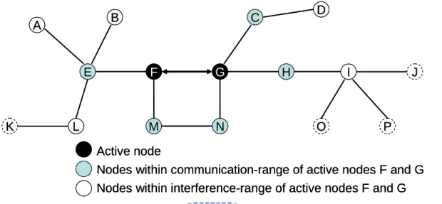
(10) 3.. If more than one NICs equipment at a node with different channel. Full duplex operation between two NIC is possible.. 4.. Channels can be assigned to NICs in a static or dynamic fashion. In a static channel assignment, every communication link is bound to a particular channel and this binding does not vary over time. In dynamic channel assignment, the binding of channel on links can vary dynamically with time.. Wired Internet. Mesh Router Mesh Client Wired Connection Wireless Connection Fig. 1. An example of wireless mesh network.. Since the interference behavior in real world is usually difficult to model, for simplify, many researches [14] assume that the interference range of a node is a k-multiple of its communication range. In this paper, we adopt the following interference model. When two node is in active state, i.e., one is transmitting data to the other, all nodes within the interference range of the two nodes using the same channel should be inactive because of the interference constrain. Fig.2 illustrates for such interference behavior model when k = 2. Each link in the figure means that its 2.

(11) incident nodes are within each other’s communication range. When link (F, G) is in active stage, links (A, E), (B, E), (C, D), (C, G), (E, F), (E, L), (F, M), (G, H) , (G, N), (H, I), (I, J), (I, O), (I, P), (K, L) and (M, N) are in inactive state.. B. A. E. K. L. D. C. F. G. M. N. H. J. I. O. P. Active node Nodes within communication-range of active nodes F and G Nodes within interference-range of active nodes F and G. Fig. 2. When node F is transmitting to node G (edge F-G is active). None of edge in this figure can be operate simultaneously, for k = 2.. In this paper, we consider the problem of routing and channel assignment in the multi-channel WMNs. Given the placement of stationary mesh routers (for convenience, we simply refer them as nodes), number of non-overlapping channels in the network, number of NICs each node is equipped with and a traffic demand profile for each node pair, assign a channel to each NIC and route the traffic according to the traffic profile such that the network performance can be maximized. The traffic profile stated above can be viewed as a collection of static traffic requests that seek to be satisfied simultaneously, or a statistical data that the future dynamic requests will follow. For the former case, the goal is to maximize the total network throughput and for the laser case, the goal is to minimize the call blocking probability.. The channel assignment problem is a NP-hard optimization problem [6] when. 3.

(12) designing a WMN. Since channel assignment problem is NP-hard, routing and channel assignment is also NP-hard. Note that for either static traffic or dynamic traffic, the channel assignment can be static or dynamic. More specifically, static channel assignment uses the same channel for a link during the operation of the network while dynamic channel assignment may change the channel of a link at any time. In our study, for the simplicity, we only focus on the static channel assignment. We provide two generic algorithms to solve static (Fig.3a) and dynamic (Fig.3b) traffic using hill climbing (HC) and simulated annealing (SA), respectively. Both HC and SA belong to iterative improvement algorithms.. A->B: 100 Kb C->D: 400 Kb E->F: 250 Kb G->H: 500 Kb I->J: 350 Kb Time Fig. 3(a). An illustration of static traffic requirement.. A->B: 64 Kb A->B: 64 Kb A->B: A->B: 64 Kb C->D: 64 Kb C->D: 64 Kb C->D: 64 Kb E->F: 64 Kb E->F: 64 Kb E->F: 64 Kb G->H: 64 Kb G->H: 64 Kb G->H: 64 Kb I->J: 64 Kb I->J: 64 Kb Time Fig. 3(b). An illustration of dynamic traffic requirement.. The rest of the paper is organized as follows. Chapter 2 describes the related work on multi-channel WMNs and gives a basic background on HC and SA. Chapter 3 presents the mixed ILP formulation for the static WMNs problem and the. 4.

(13) algorithms for the static routing and channel assignment. Chapter 4 shows the simulation results. Conclusion is given in Chapter 5.. 5.

(14) Chapter 2: Related work In this chapter, we review some of the previous work on the routing and channel assignment problems in WMNs. A survey paper [8] presents a detailed study on recent advances and open research issues in WMNs. Chapter 2.1 discusses the interference model and the capacity problem in multi-hops wireless network [7] [9] [15] [16] [17] [18] [19] [20]. Chapter 2.2 briefly describes the main ideas of the algorithms proposed in [1] [2] [3] [4] [5] [6] [10] [11] [21] that solve the routing and channel assignment problems in WMNs. In the end of the chapter, we give a basic background on HC and SA.. 2.1 Interference Model and Capacity for WMNs. Interference is the major factor of multi-hops wireless capacity. Due to spatial contention for the shared wireless medium, not all nodes can concurrently transmit packet to each other in the network. The IEEE 802.11 standard using RTS (Request-to-send)/CTS (Clear-to-send) mechanism to avoid the occurrence of parallel transmission. These messages are typically heard by all others nodes within radio range of either (or both) neighbors, and contain information that informs all the nodes of the duration of the data transmission will last.. Authors in [7] introduce the bottleneck collision domain, defined as the geographical area of the network that bounds from above the amount of data that can be transmitted in the network. It define the collision domain of a link (a, b) as a set of links formed by link (a, b) and all other links that have to be inactive for link (a, b) to. 6.

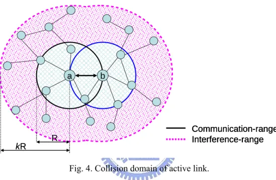
(15) transmit successfully. According to all traffic requests, the expected load of each link can be obtained, then using collision domain concept the bottleneck collision domain and the nominal capacity can be determined. Many researches define that collision domain as k-multiple as communication range within both transmit node and receive node (show in Fig.4).. a. b. Communication-range Interference-range. R kR. Fig. 4. Collision domain of active link.. In [9], the authors consider routing and CAP into scheduling problem in multi-hop wireless network, under three increasingly constraining interference models and characterize the network throughput in each of these models. It also express the necessary conditions for achievability in these three models as linear constraints, and exploit the structure of these constraints to develop efficient fully polynomial time approximation algorithms that route end-to-end flows between multiple source destination pairs. Another parallel work [10] proposes a network model that captures the key practical aspects of such systems and characterizes the constraints binding their behavior. It address the capacity planning question, and develop algorithms to jointly optimize the routing, link channel assignment and scheduling in order to obtain 7.

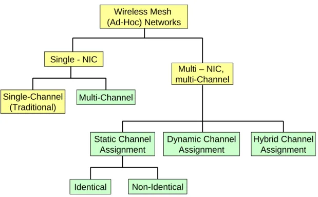
(16) upper and lower bounds for the capacity region under a given objective function.. 2.2 Channel Assignment Strategies for Multi-Channel WMNs Channel assignment problem of multi-channel in WMN can be classified as shown in Fig.5. Basically, WMNs can be categorized depending on whether a node in the network could have only single NIC or multiple NICs. The latter can be further classified into three sub-classes, static assignment, dynamic assignment and hybrid assignment. We will discuss the difference between them following.. Wireless Mesh (Ad-Hoc) Networks. Single - NIC Multi – NIC, multi-Channel Single-Channel (Traditional). Multi-Channel. Static Channel Assignment. Identical. Dynamic Channel Assignment. Hybrid Channel Assignment. Non-Identical. Fig. 5. Classification of channel assignment strategies.. 2.2.1 Single Network Interface Card. In such network, each node has only one NIC. It can perform by each timeslot. 8.

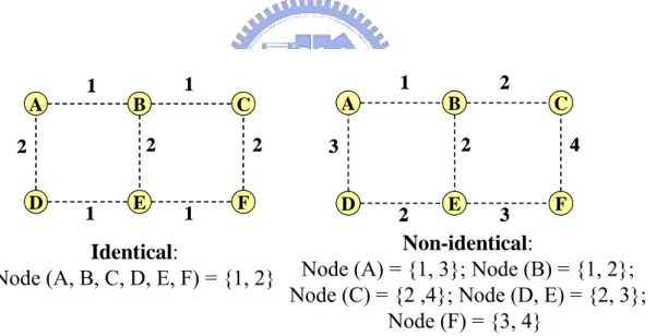
(17) switching on available channel to avoid the decreasing of bandwidth caused by interference [1] [21]. Bahl et al. [1] propose SSCH, a link-layer solution, to increase the capacity of IEEE 802.11 network by utilizing frequency diversity. Each node using SSCH switches across channels in such a manner that node desiring to communicate overlap, while disjoint communication mostly do not overlap, and hence do not interfere with each other. The ability to switch an interface’s channel to another is a beneficial for cost reduction compared with equipping a node with multiple NICs. However, the control messages for synchronization requirements for data communication and the interface switching delay may cause much overhead to the network.. 2.2.2 Multiple Network Interface Card. Equipping a node with multiple NICs, on the contrary, can offer better performance than the single NIC solution at the expense of higher network cost. The channel assignment strategies can be classified into three sub-classes. A.. Static Assignment: Static channel assignment strategies [2] [5] [6] [10] assign each interface to a channel either permanently, or for “long intervals” of time and it is well-suited for use when the interface switching delay is large. Besides, static assignment strategies do not require special coordination among nodes. It can be further classified into two types: identical and non-identical (see Fig.7). In identical approach, interfaces of each node in the network are assigned to a common set of channels. Draves et al. [2] have proposed LQSR, a source routing protocol for multi-channel multi-interface networks. They present a new combined path metric WCETT to choose a high-throughput path between a source and a destination, and ensures “high-quality” routes are selected. 9.

(18) However, this algorithm is under the assumption that the number of NICs is equal to the number of channels used by the network. In non-identical approach, NICs of different nodes may be assigned to different set of channels and the number of available NICs can be less than the number of available channels. In [5] [6], distributed and centralized heuristic channel assignment algorithms, respectively, are proposed for bandwidth allocation and load-balance routing algorithms. The main idea is to separate the interference region more efficiently to obtain more available bandwidth. Authors in [10] propose Balanced Static Channel Assignment (BSCA) that using an (almost) greedy approach in solving the static channel assignment problem. The main idea behind the BSCA algorithm is to ensure that none of the constraint sets are loaded by any channel.. 1. 1. 1 A. B 2. 2 D. 1. E. A. C 2. 1. Identical: Node (A, B, C, D, E, F) = {1, 2}. C. 2. 3. F. 2 B. D. 2. E. 4. 3. F. Non-identical: Node (A) = {1, 3}; Node (B) = {1, 2}; Node (C) = {2 ,4}; Node (D, E) = {2, 3}; Node (F) = {3, 4}. Fig. 6. Identical and non-identical channel assignment.. B.. Dynamic Assignment: Dynamic channel assignment is more flexible than static one since it has the ability to switch NICs to any channel that has the lowest interference during different time slots [1] [10]. When more NICs equipped, the aggregate bandwidth increase because of the collateral transmission of each node. In [10], the authors propose Packing Dynamic Channel Assignment (PDCA) that. 10.

(19) performs link channel assignment and scheduling simultaneously. The main idea behind the PDCA algorithm is to pack the flows in a greedy manner in each time period.. C.. Hybrid Assignment: Hybrid channel assignment strategies combine static and dynamic channel assignment strategies by applying a static assignment for some interfaces and a dynamic assignment for other interfaces [3] [4] [13] [18]. One intuition opinion is applying each node with a common channel approach for control purpose [13] and uses this common channel to coordinate dynamic interfaces. Using this method, it can change channel assignment more flexible and frequent. In [3] [4], the authors propose another channel assignment strategy that each node has one NIC assigned to specific fixed channel (in [13], all nodes assigned to common channel) and the others are switchable. This fixed NIC is always listening to specific channel called listening channel. All nodes within network need to record a table of listening channel of each neighbor node. When node A has to send a packet to node B, A switches its switchable interface to B’s listening channel and transmits the packet. Hybrid channel assignment strategies allow simplified coordination algorithms supported by static assignment while retaining the flexibility of dynamic assignment.. 2.3 Hill Climbing and Simulated Annealing 2.3.1 Hill Climbing. Hill climbing algorithm, or alternatively, gradient descent, is an iterative method that continually moves in the direction of goal. For conveniently, we can start from 11.

(20) various starting points and each starting point running HC algorithms to find a so-called local minimum cost solution (see Fig.7a). Clearly, if enough start points and iterations are allowed, HC will eventually find the optimal solution.. Cost. Final Solution. Time Time Fig. 7(a). HC iteration at each time for the best solution.. 2.3.2 Simulated Annealing. Simulated annealing is similar to HC. The main difference is that SA allows cost upwards step with altering accepted probability at every iteration (see Fig.7b). Generally, an optimization problem consists of a set S of configurations space (solution) and cost function Co which determines for each configuration s the cost Co(s). Before enter next step, we need to calculate next configuration space s’ which is derived by a neighborhood structure N on S. N(s) determines for each solution s a set of possible transitions which can be proposed by s. If we replaced s with s’ only when Co(s’) < Co(s), the result terminates in a local minimum (the same as HC algorithm). To avoid trapping in such poor local optima, SA occasionally allows selecting configuration s’ with higher Co(s’) according to the so-called Metropolis criterion. More specifically, the SA continues with the configuration s’ with a probability given by P = min{1, exp(-(Co(s’) - Co(s)) / t)}, where t is a positive control parameter representing temperature in the physical annealing process. 12.

(21) Furthermore, there exists a random number r between 0 and 1.. If P > r, the. configuration s’ will be accepted. Note that the P increases with the increasing of temperature t or the decreasing of Co(s’)-Co(s). If cost decreasing, the s’ is always accepted. The HC and SA algorithm is shown in Fig.8a and Fig.8b.. tx. Cost. ty. Final Solution. Time Fig. 7(b). SA allowing cost uphill moves up at each time t for global optima.. Step 1: Initialize ( s ← s start ) Step 2: Generate s’ from N(s) Step 3: If Co(s’) < Co(s) then s ← s ' else continue with old s Step 4: If NO_BETTER_FOUND go next , else go to Step.2 Step 5: Finish, return s Fig. 8(a). Formal procedure of Hill Climbing.. Step 1: Initialize ( s ← s start , t 0 ), k ← 0 Step 2: Generate s’ from N(s) Step 3: If min{1, exp(-(Co(s’)-Co(s)) / t k )} > random[0:1] then s ← s ' else continue with old s Step 4: k ← k + 1 Step 5: Compute t k for next iteration Step 6: If t k ≈ 0 go next , else go to Step.2 Step 7: Finish, return s Fig. 8(b). Formal procedure of Simulated Annealing. 13.

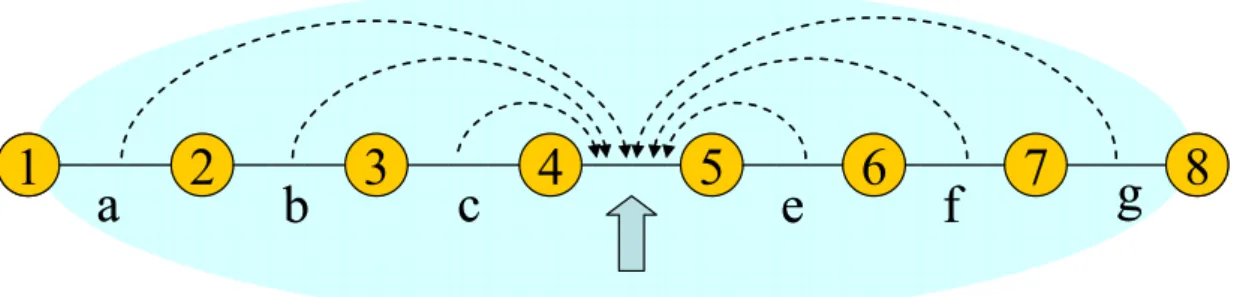
(22) Chapter. 3:. Proposed. Routing. and. Channel. Assignment Algorithms 3.1 The Variables and Objective Function. A WMN is presented as a directed graph G = (V, E) where V represents the set of nodes in the network, E the set of links that can deliver data (we assume the links are directional). Note that link (i, j ) ∈ E implies that i is within the communication. range of j. We assume the number of NICs to be the same across all nodes and denote constant members as follows: C. Capacity per channel. t s ,d. Traffic requirement for node pair (s, d). NIC. Number of interfaces for each node. CHL. Number of non-overlap channel. The variables are defined as follows:. t ' s ,d. Amount of traffic successfully routed for node pair (s, d). The ultimate goal of traffic routing and channel assignment in the network is to maximize the overall throughput. The objective of network plan is defined as. Objective:. maximize∑ t's,d s,d. (1). When the capacity C is given, Fig.9 illustrates the maximum available capacity of specific link, assuming that all the links use the same channel. The letter under each link represents the load on that link. The maximum available capacity of link (4, 5) is calculated by C minus the total load within interference. Note that if this 14.

(23) subtraction results in a negative value, the available capacity of link (4, 5) is zero.. 1. a. 2. b. 3. c. 4. 5. e. 6. f. 7. g 8. Fig. 9. Available capacity on link (4, 5) is Max{C – (a + b + c + e + f + g), 0}. If all links are using the same channel.. 3.2 Load Aware Single Request Routing Algorithm. The heuristic provided in this section is for routing a single request and assign the channels that called Load Aware Single Request Routing Algorithm (LASRR), if necessary, on its route. It is used by both HCRCA algorithm and SARCA algorithm that we propose later. The current network configuration, in which some links may have not yet been assigned, and a traffic request are given, and the algorithm will determine the route and channel assignment of the links along the route for the request without modifying the existing assignment.. First, we compute the available capacity of each link according to the current channel assignment and current load on each link. If the maximum available capacity of the links is less than the demand flow and the link will be removed temporarily. Consequently, we derive a new graph that each link has enough bandwidth to accommodate the request. Then we use shortest path algorithm (e.g., dijkstra etc.) to compute all shortest paths from source node to destination node and collect the first 15.

(24) links of all shortest paths. One of these links is chosen and assigned a channel according to a specific selection, e.g., least-bandwidth-first, large-bandwidth-first, etc. Then, we assign channel to NICs of connected node and update link’s load (similar to update the maximum available bandwidth within the interference-range using the same channel).. Repeatedly, the request may end up at the destination, thus satisfied. Otherwise the request fails to be routed because of the insufficient bandwidth. The algorithm is summarized in Fig.10a.. Load Aware Single Request Routing Algorithm (LASRR): Input: G(V, E) Network topology C Capacity pre channel. t s ,d. A traffic requirement for node s to d Current channel assignment Current load on each link. Output: 1. New channel assignment 2. New load on each link 3. t 'sd Algorithm: Step 1: a ← s .. Step 2: Calculate the available capacity of each link and remove links that fit in one of the following conditions: (also see Fig.10b) a. if NICa = 0 & NICb = 0 and 1. Ca (a ) ∩ Ca (b) = {φ} or w 2. capacityab < t s ,d , ∀ w ∈ Ca (a ) ∩ Ca (b) w b. if NICa = 0 & NICb > 0 and capacityab < t s ,d , ∀ w ∈ Ca (a) w c. if NICa > 0 & NICb = 0 and capacityab < t s ,d , ∀ w ∈ Ca (b) w d. if NICa > 0 & NICb > 0 and capacityab < t s ,d , ∀ w. 16.

(25) where. NICa represent the number of non-assigned NIC in node a w capacityab represents the available capacity on link (a, b) using. channel w. Ca (a) : set of channels already assigned to NICs in node a Determining the set of first links of all shortest paths from a to d. Select a link determined from Step 3 with the maximum weight(l, w), where weight(l, w) represents the function for selection criterion on link l using channel w. Update the channel assignment and the load on this link. Node a move on one step. If a!= d go to Step 2; else go to Step 7. Finish.. Step 3: Step 4:. Step 5: Step 6: Step 7:. Fig. 10(a). Load aware single request routing algorithm (LASRR).. a. NICa = 0 & NICb = 0： 1.. 3. x. 1. a. b. Ca (a) ∩ Ca(b) = {φ} 1. a. 1. 3. b. d. NICa > 0 & NICb > 0：. c. NICa > 0 & NICb = 0： 3. ALL. 4. 2. 2.. b. NICa = 0 & NICb > 0：. 1. a. 1, 2. a b. 4. b. 2. 2. Ca(a) ∩ Ca(b) = {1,2,..., CHL} 1. 2. capacity1 < tsd. capacity1 < tsd …. Ca(a) ∩ Ca(b) = {1}. Ca(a) ∩ Ca(b) = {1,2} capacity1 < tsd & capacity2 < tsd. & capacityCHL < tsd. Fig. 10(b). Criterion of non-conform links (if NIC=2 for all nodes). Italic number represents the channel already assigned on the link; Bold represents the available channel on link (a, b).. 3.3 Hill Climbing Based Routing and Channel Assignment. In this section, we introduce our approach, called hill climbing based routing and channel assignment algorithm (HCRCA), to solve the routing and channel assignment problem for static traffic. Hill climbing is a generic algorithm used for solving 17.

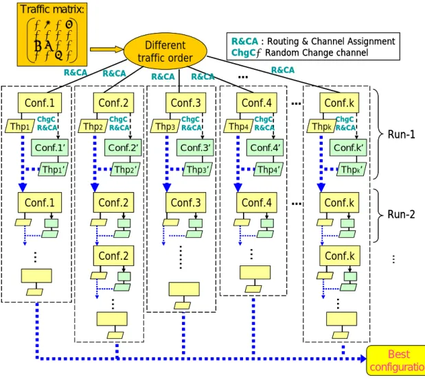
(26) optimization problem. The main idea is to start at some different initial configurations. Each configuration may contain several runs to find a best solution until a pre-defined terminal condition is reached.. First, an initial configuration is derived as follows. The traffic requests are sorted into sequence according to a specific metrics. Then each request is routed in that sequence using LASRR algorithm described in previous section. When finished, we derive an overall throughput in this configuration. Note that if different sorting sequence is used, different overall throughput is obtained. In each run, a new configuration will be generated by slightly shuffling the current channel assignment and then route the requests in the same order as is done previously. The new overall throughput is then compared with the original one and the better is reserved for the next run. The runs continue until ρ consecutive runs have the same overall throughput. The above procedure is for the completion of one single initial configuration and one may generate numbers of different initial configurations to be completed and output the best of them. Clearly, to obtain satisfactory result, one may either set ρ to a large enough number or generate a large set of initial configurations. An overview of HCRCA algorithm is shown in Fig.11.. 18.

(27) Traffic matrix: 0 a 0 c 0 0 0 0 e d 0 0 0 0 b 0 R&CA. Conf.1 Thp1. ChgC R&CA. R&CA : Routing & Channel Assignment ChgC：Random Change channel. Different traffic order R&CA. Conf.2 Thp2. ChgC R&CA. R&CA. R&CA. Conf.3 Thp3. R&CA. …. Conf.4. ChgC R&CA. Thp4. …. ChgC R&CA. Conf.k Thpk. ChgC R&CA. Conf.1’. Conf.2’. Conf.3’. Conf.4’. Conf.k’. Thp1’. Thp2’. Thp3’. Thp4’. Thpk’. Conf.2. Conf.3. Conf.4. .... Conf.2. ....... .... …. Conf.k. Run-2. Conf.k. .... Conf.1. Run-1. .... .... Best configuration. Fig. 11. Hill climbing based routing and channel assignment algorithm.. 3.4 Simulated Annealing Based Routing and Channel Assignment. In this section, we propose a dynamic traffic model and use it for multi-hops WMN transmission focus on multimedia application. By using the concept of simulated annealing algorithm, simulated annealing based routing and channel assignment algorithm (SARCA) is proposed to solve the channel assignment problem. Then using SARCA, we can get a channel assignment that may have the best potential capacity (lowest interference). Once link channel assignment is done, we. 19.

(28) using LASRR to route traffic. Unlike static traffic that each traffic request, dynamic traffic means that traffic request have both arrival and departure time. When a traffic request arrives, we need to find a routing path with enough bandwidth and update resource capture by this traffic request or it will be blocked. When a traffic request leaves, the resource must be released.. The parameter call_size represent the bandwidth (kbps) demand of a multimedia requirement and we assume the bandwidth of each call request is the same. Then we simplify transform the maximum capacity C into multimedia calls concept where. λmax represent the maximum call can be established between two nodes:. λmax = C / call _ size. (2). We also create the call requirement matrix λs,d (replaced by the original t s ,d ) for node pair (s, d) of dimension n x n. Each λs,d represent the number of calls requirement between node s and d during an unit time and is randomly chosen between 0 to λM ( λM ≤ λmax ) and the average call number (symbol as λavg ) is approximate to λM / 2 . The traffic request for node pair (s, d) is represented as. t s , d = λs , d × call _ size. (3). Afterward, call requests are assumed to arrive according to an independent Poisson process with arrival rate λs,d . Service time of each request is exponentially distributed with mean. 1. μ. (in the simulations average service time is set to 1 time. unit).. We use SARCA to solve the channel assignment problem of dynamic traffic. 20.

(29) requirement in WMNs. Generally, it consists of a set S of configurations space (solution) and cost function Co which determines for each configuration s the cost Co(s). Before enter next step, we need to calculate next configuration space s’ which. is derived by a neighborhood structure N on S. N(s) determines for each solution s a set of possible transitions which can be proposed by s. Another important parameter t represents the temperature, where t is a positive control parameter, which is gradually decreased to zero during the execution of the algorithm. A formal procedure of SA to optimization problems was proposed in Fig.8b.. In order to apply SA to channel assignment problem, we have to formulate channel assignment problem as a discrete optimization problem. For the reason, we need to define the corresponding discrete configuration space S, the cost function Co and the neighborhood structure N.. A. Configuration Space (S): We simplify define our configuration s as a set of channel assignment for each link in the network. A channel matrix ( chli , j ) of dimension n x n with the following interpretation of solution entries of channel assignment,. ⎧ 0 if (i, j) ∉ E chli , j = ⎨ ⎩ w Channel assigned to link (i, j). (4). where w is the channel number between 1 to CHL. Otherwise, channel number 0 represents that two nodes do not within communication-range each other.. B. Cost Function (Co): Cost function decides that how much potential bandwidth it have according to a. 21.

(30) configuration and the given traffic matrix. Prior to defining Co, we introduce link load estimation and a link capacity estimation method referred in Raniwala et al.. [6]. The estimation of expected link load is based on the notion of link criticality. The expected link loads are initialed by assuming perfect load balancing across all paths between each traffic request pair. P( s, d ) denotes the number of acceptable paths betweens node pair (s, d) and Pl ( s, d ) denotes the number of acceptable paths that pass link l. Then the expected-load on link l, φl , is calculated using the equation. φl =. ∑ s,d. Pl ( s , d ) × ts,d P (s, d ). (5). Given a specific configuration s (channel assignment) and expected-load on each link, we can compute the expected-capacity by using a ratio distribution method. The link capacity bwl for a link l is determined by the ratio of expected load φl to the total load in the interference-range l that uses the same channel as l. That is,. bw l =. ∑. φl. φ j∈range ( l ) j. ×C. (6). where range(l) represents the set of links within interference-range for link l that use the same channel as link l. After calculated the expected-load ( φl ) and expected-capacity ( bwl ) information for each link l, links are classified into under-assignment links and over-assignment links. A link l is a Under-assignment link if the expected-capacity of l is less than the. expected-load ( φl > bwl ). Otherwise, it is an over-assignment link. We define a cost function as. Co ( s ) = α ⋅ (. ∑φ. l ∀l ,φ l > bwl. − bwl ) − β ⋅ (. ∑ bw − φ ). ∀l , bwl ≥φ l. l. l. (7). where 0 ≤ α ≤ 1 and 0 ≤ β ≤ 1. For example, if α = 1, β = 0 and C(s) = 0, it means this configuration can satisfy all t s ,d theoretically. 22.

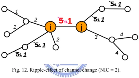
(31) C. Neighborhood Structure (N): Designing a neighbor structure N from configuration space s in multi-channel WMNs is not as easy as in cellular networks [12] because of the node NIC constraint. For example, in Fig.12, if we change channel on link (i, j) from chnl-5 to chnl-1, NICs on node i and node j are needed to adapt their channel in order to keep the connectivity of network. However, it may cause what we called ripple-effect of channel changing on the adjacent links that use the same channel as link (i, j). Usually, this may deteriorate the interference and thus raises Co(s).. 5 1 1 2. i. 1. 5 1. 5 1. 5 1. j 4. 3. 2. 4. 5 1. Fig. 12. Ripple-effect of channel change (NIC = 2).. Since expected-load of the links on the network never change, expected-capacity of links depend on how channels are assigned to the links. Two methods to increase the expected-capacity on link l are proposed. 1.. Change original channel on link l to another channel that causes less interference.. 2.. Change the channel of links in range(l) (except for l) that use the same channel as l to decrease interference.. Now, we describe how neighborhood structure N(s) is generated. First, a critical link is selected (e.g., by random or largest under-assigned etc.). Secondly, execute capacity-release procedure shown in Fig.13. 23.

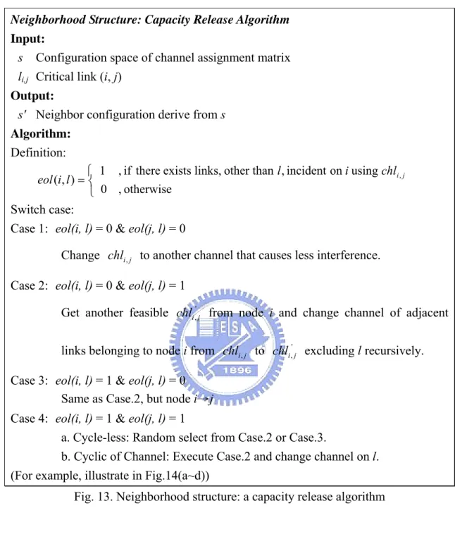
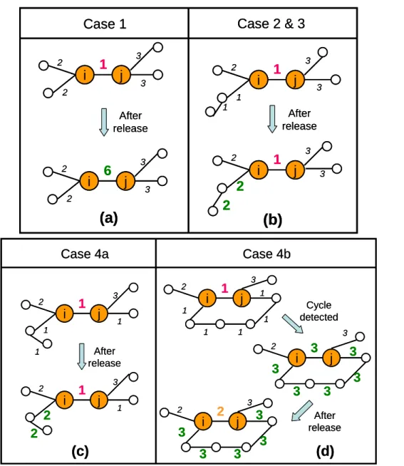
(32) Neighborhood Structure: Capacity Release Algorithm Input: s Configuration space of channel assignment matrix li,j Critical link (i, j) Output: s' Neighbor configuration derive from s Algorithm: Definition: ⎧ 1 , if there exists links, other than l , incident on i using chli , j eol (i, l ) = ⎨ ⎩ 0 , otherwise Switch case:. Case 1: eol(i, l) = 0 & eol(j, l) = 0 Change chli , j to another channel that causes less interference. Case 2: eol(i, l) = 0 & eol(j, l) = 1 Get another feasible chli ,' j from node i and change channel of adjacent links belonging to node i from chli , j to chli ,' j excluding l recursively. Case 3: eol(i, l) = 1 & eol(j, l) = 0 Same as Case.2, but node i→j Case 4: eol(i, l) = 1 & eol(j, l) = 1 a. Cycle-less: Random select from Case.2 or Case.3. b. Cyclic of Channel: Execute Case.2 and change channel on l. (For example, illustrate in Fig.14(a~d)) Fig. 13. Neighborhood structure: a capacity release algorithm. 24.

(33) Case 2 & 3. Case 1 3. 1. 2. i. 2. j. i. 3. 2. 3. 1. j. 3. 1 1. After release. 2. j. i. Case 4b 2 3. j. i. 3. 1. 1. j. 1. 1 1. 1. 3 2. After release. 1. 2. i 2. 3. 3. j. 1. 3. i. 2. (c). i. 2. 3. 3. 3. j. 3. After release. 3 3. j. 3 3. 3. 2. Cycle detected. 1. 1 1. 3. (b). Case 4a. i. j. 2. (a). 1. 3. 2. 3. 2. 2. 1. 2. 3. 6. i. After release. 3. (d). Fig. 14. Examples of capacity release algorithm.. D. Cooling Schedule: The probability of accepting a worse state is a function of both the temperature (t) of the system and the change in the cost function. As the temperature decreases, the probability of accepting worse moves decreases. If t = 0, no worse moves are accepted (i.e. hill climbing algorithm). Initial temperature ( t 0 ) must be high enough to allow moves to almost neighbor state or we are in danger of implementing hill climbing. And it is important that it should allow enough iteration at each temperature so that. 25.

(34) the system can reach the stable state. We refer to the cooling schedule in [12] and define temperature decrement rule:. t k +1 = t k ⋅ exp(−. λt ) σ. (8). The decrease ΔC in average cost between two iteration should be less than the standard deviation of the cost: def. ΔC = C (t k +1 ) − C (t k ) = −λσ , with λ ∈ (0,1). (9). In practice, it is not necessary to let the temperature reach zero because the chances of accepting a worse move are almost the same as the temperature being equal to zero. Therefore, the stopping criteria can either be a suitably low temperature or when the system is "frozen" at the current temperature (i.e. no better or worse moves are being accepted (equal to hill climbing algorithm).. After the termination of SARCA, the network is ready to serve the dynamic coming request using LASRR. With the best configuration (channel assignment) calculate above, we can decrease blocking probability of routing arrival traffic theoretically.. 26.

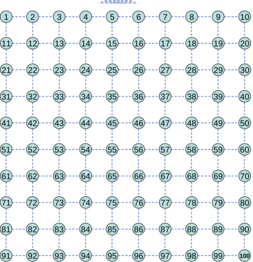
(35) Chapter 4: Simulation Results In this chapter, we present the results of our performance evaluation based on simulations. To ensure that the simulation results were comparable to others, the simulation environment was modeled on that in [6] and the number of NICs per node to be the same across all nodes. In all the simulation, we consider a full 10x10 grid topology with 100 nodes (see Fig.15) that each node has at most 4 neighbors in the grid topology. We assume that the length of interference-range is 2-multiple than communication-range (k = 2) and each link can be assigned one channel. Therefore, a node equipped with more than 4 NICs is redundant.. 1. 2. 3. 4. 5. 6. 7. 8. 9. 10. 11. 12. 13. 14. 15. 16. 17. 18. 19. 20. 21. 22. 23. 24. 25. 26. 27. 28. 29. 30. 31. 32. 33. 34. 35. 36. 37. 38. 39. 40. 41. 42. 43. 44. 45. 46. 47. 48. 49. 50. 51. 52. 53. 54. 55. 56. 57. 58. 59. 60. 61. 62. 63. 64. 65. 66. 67. 68. 69. 70. 71. 72. 73. 74. 75. 76. 77. 78. 79. 80. 81. 82. 83. 84. 85. 86. 87. 88. 89. 90. 91. 92. 93. 94. 95. 96. 97. 98. 99. 100. Fig. 15. A 10x10 grid topology with 100 nodes.. 27.

(36) 4.1 Simulation Result of HCRCA – Static Traffic. The objective function in static traffic requirement using HCRCA algorithm is to maximize the overall throughput that is defined as the sum of feasible bandwidth assigned between all traffic request pair. We demonstrate the performance improvements. of. HCRCA. algorithm. compare. with. load-aware. channel. assignment/routing algorithm proposed in [6]. We perform an extensive simulation study using NS-2 simulator with modifying by above-mentioned author to support multiple NICs on mobile nodes.. Fig.16 presents the comparison of overlap throughput over different algorithms that each node equipped with 2 NICs and the number of non-overlap channel is 12. This testing includes 10 randomly generated traffic profiles and each traffic profile contains 20 randomly chosen traffic pairs (source-destination nodes). For each traffic pair, the amount of traffic request between source-destination pair was chosen randomly between 0~3 Mbps (average = 1.5 Mbps). Fig.17 and Fig.18 shows the same performance comparison when the number of NICs is change to 3 and 4. In order to guarantee the saturated of network throughput, the number of traffic request pairs per profile is also change from 20 to 30 and 40.. For clearly, in Fig.19, we calculate the average overall throughput presented in Fig.16, 17 and 18. Compared with conventional single-channel WMNs and load-aware. channel. assignment. algorithms,. HCRCA. algorithm. achieves. approximately 10 times improvement over single-channel WMNs and about 30% improvement over load-aware channel assignment algorithm when using 2 NICs per node. In practice, equipping each mesh node with more NICs can obtain excellent 28.

(37) performance against to single-channel WMNs (about 17 times improvement for 3 NICs per node and 22 times improvement for 4 NICs per node). Moreover, the performance of HCRCA is still superior to load-aware channel assignment algorithm when more than two NICs are available.. In Fig.20, we compare the performance with two algorithms by using different traffic request pairs that each node pair was chosen at random between 0~3 Mbps and each node equipped with 2, 3 and 4 NICs. As more traffic request pairs introduced, the traffic flow is more distributed across the network leading to the increasing of network utilization. When the traffic request pairs are increasing, the overall throughput becomes convergence. Then, we can estimate the saturated throughput with different NICs number in this network.. Fig. 16. The overall network throughput with 2 NICs per node.. 29.

(38) Fig. 17. The overall network throughput with 3 NICs per node.. Fig. 18. The overall network throughput with 4 NICs per node.. 30.

(39) Fig. 19. The average network overall throughput with 2-3-4 NICs per node.. Fig. 20. Impact of different traffic request pairs and number of NICs on overall throughput improvements. 31.

(40) 4.2 Simulation Result of SARCA – Dynamic Traffic. The objective function in dynamic traffic requirement using SARCA algorithm is to minimize the overall blocking probability of all arrival events. In order to compare the performance of SARCA algorithm with the other one, we retain the channel assignment derive from the load-aware channel assignment/routing algorithm and modify it to support arrival/departure event of each traffic request. We using VoIP call as our multimedia application and assume call_size = 64 Kbps. The traffic profile is randomly chosen 100 call (traffic) request pairs and the amount of each call request between source/destination pair was chosen at random range 0~ λM ( λM ≤ λmax ). The overall-call-request is the sum of all λsd that represent the total arrival call requests. during a unit time. For example, if λavg = 2, it means that there are 200 (2 x 100) calls request arrival during a unit time.. Fig.21 shows the comparison of blocking probability using two algorithms that each node equipped with 2 NICs. Note that in this figure, when λavg = 2, the blocking probability of our SARCA algorithm is approximate to 0%. It means that all arrival requests can be satisfied because of the sufficient bandwidth (resource) in network or the less value of overall-call-request. As more λavg value is introduced, the blocking probability increasing quickly because the insufficient for network bandwidth.. In Fig.22, when 3 NICs equipped, the overall performance is better than 2 NICs obviously (note the different x-scale from Fig.20). Our SARCA algorithm can achieve lower blocking probability than load-aware channel assignment/routing algorithm. If 32.

(41) the tolerable blocking rate is below 20%, SARCA can reach λavg = 11, and another algorithm can only reach λavg = 9 relatively. In Fig.23, when 4 NIC each node is available, the performance is further improved than previous two evaluations.. Fig.24, Fig.25 and Fig.26 show the throughput (arrival/departure) curve for each. λavg value in Fig.21, Fig.22 and Fig.23. The x-axis represents the process of simulation time and y-axis represents the number of calls stay on the network. Note that in the beginning, the arrival of sustained call requests form of a rising curve. Afterward, the number of calls stay on network will balance between arrival/departure of requests and residual bandwidth. Finally, call request depart gradually and form of a falling curve.. (λavg ). Fig. 21. The overall network blocking probability with 2 NICs per node.. 33.

(42) Fig. 22. The overall network blocking probability with 3 NICs per node.. Fig. 23. The overall network blocking probability with 4 NICs per node.. 34.

(43) (a) λavg = 2. (b) λavg = 2.5. (c) λavg = 3. (d) λavg = 3.5. (e) λavg = 4. (f) λavg = 4.5. Fig. 24. The network throughput curve with 2 NICs per node. 35.

(44) (a) λavg = 7. (b) λavg = 8. (c) λavg = 9. (d) λavg = 10. (e) λavg = 11. (f) λavg = 12. (g) λavg = 13. (h) λavg = 14. Fig. 25. The network throughput curve with 3 NICs per node.. 36.

(45) (a) λavg = 9. (b) λavg = 10. (c) λavg = 11. (d) λavg = 12. (e) λavg = 13. (f) λavg = 14. (g) λavg = 15. (h) λavg = 16. Fig. 26. The network throughput curve with 4 NICs per node.. 37.

(46) Chapter 5: Conclusions Despite the advances in wireless physical-layer technologies, interference is still the main factor of the decreasing in wireless network bandwidth. However, when multiple channels are available, equipping each mesh node with multiple NICs allows the network to use different radio channels simultaneously. Then the available bandwidth can be increased because of the decreasing of interference.. In the study, we propose two algorithms called hill climbing based routing and channel assignment (HCRCA) and simulated annealing based routing and channel assignment algorithms (SARCA) to solve routing and channel assignment problem for static traffic and dynamic traffic, respectively. According to give a graph topology, number of non-overlapping channels, NICs of each node, HCRCA aims to maximize the overall network throughput. Contrary to HCRCA, SARCA is for dynamic traffic requirement with the goal of minimizing the call blocking probability, by approximating an optimal channel assignment which may have maximum potential available capacity. We demonstrated through simulations that the performance improvement of our algorithms.. The simulation results certified the superiority of our algorithms. Fig. 19 shows that our HCRCA algorithm has better performance than load-aware CA algorithm, when equipped with 2 NICs each node, the improvement is approximate to 30%. In Fig.20, with more traffic request pairs, HCRCA still outperforms the previous algorithm. In Fig.21~23, when dynamic traffic requirement is introduced, our SARCA algorithm can also achieve lower blocking probability respectively.. 38.

(47) Reference: [1] P. Bahl, R. Chandra and J. Dunagan, "SSCH: Slotted Seeded Channel Hopping for Capacity Improvement in IEEE 802.11 Ad-Hoc Wireless Networks", ACM Mobicom, Sept. 2004.. [2] R. Draves, J. Padhye, and B. Zill, "Routing in Multi-radio, Multi-hop Wireless Mesh Networks", ACM Mobicom, Sept. 2004. [3] P. Kyasanur and N. Vaidya, "Routing and Interface Assignment in Multi-Channel Multi-Interface Wireless Networks", IEEE WCNC, 2005. [4] P. Kyasanur and N. Vaidya, "Routing in Multi-Channel Multi-Interface Ad Hoc Wireless Networks", Technical Report, Dec. 2004. [5] A. Raniwala and T. Chiueh, "Architecture and Algorithms for an IEEE 802.11-Based Multi-Channel Wireless Mesh Network", IEEE Infocom, March 2005. [6] A. Raniwala, K. Gopalan and T. Chiueh, "Centralized Algorithms for Multi-channel Wireless Mesh Networks", ACM Mobile Computing and Communications Review, April 2004.. [7] J. Jun and M. L. Sichitiu, "The Nominal Capacity of Wireless Mesh Networks", IEEE Wireless Communications, Vol.10, No.5, pp.8-14, Oct 2003.. [8] I. F. Akyildiz, X. Wang, and W. Wang, "Wireless mesh networks: A survey", Computer Networks Journal (Elsevier), March 2005.. [9] M. Kodialam, and T. Nandagopal, "The Effect of Interference on the Capacity of Multi-hop Wireless Networks", IEEE Symposium on Information Theory, June 2004.. 39.

(48) [10] M. Kodialam, and T. Nandagopal, "Characterizing the Capacity Region in Multi-Radio Multi-Channel Wireless Mesh Networks", ACM Mobicom, 2005. [11] P.. Demestichas,. E.. Tzifa,. M.. Theologou. and. M.. Anagnostou,. "Interference-oriented carrier assignment in wireless communications", IEEE Communications Letters, Vol.7, No.1, pp.7-9, Jan. 2003.. [12] M. Duque-Anton, D. Kunz and B. Ruber, "Channel Assignment for Cellular Radio Using Simulated Annealing," IEEE Transactions on Vehicular Technology, Vol.42, No.1, pp.14-21, Feb 1993. [13] S.L. Wu, C.Y. Lin, Y.C. Tseng, and J.P. Sheu, “A New Multi-Channel MAC Protocol with On-Demand Channel Assignment for Multi-Hop Mobile Ad Hoc Networks,” in International Symposium on Parallel Architectures, Algorithms and Networks (ISPAN), 2000.. [14] M. A. Alicherry, R. Bhatia, and L. Li, “Joint Channel Assignment and Routing for Throughput Optimization in Multi-radio Wireless Mesh Networks”, ACM Mobicom, 2005. [15] M. Kodialam, and T. Nandagopal, "Characterizing Achievable Rates in Multi-hop Wireless Networks : The Joint Routing and Scheduling Problem", ACM MobiCom, September 2003.. [16] M. K. Marina and S. R. Das, "A Topology Control Approach for Utilizing Multiple Channels in Multi-Radio Wireless Mesh Networks,", Broadnets 2005. [17] K. Jain, J. Padhye, V. Padmanabhan, and L. Qiu, "Impact of Interference on Multi-hop Wireless Network Performance", in Proc. IEEE/ACM MobiCom, 2003. [18] P. Kyasanur and N. Vaidya, "Capacity of Multi-Channel Wireless Networks: Impact of Number of Channels and Interfaces", in ACM Mobicom, August 2005. 40.

(49) [19] H. Balakrishnan et al., "The Distance-2 Matching Problem and Its Relationship to the MAC-Layer Capacity of Ad Hoc Wireless Networks", IEEE JSAC, vol. 22, no. 6, 2004 [20] P. Gupta, P.R. Kumar, "The Capacity of Wireless Networks", IEEE Transactions on Information Theory, vol. 46, no 2, 2000. [21] J. So, N. Vaidya, "Multi-Channel MAC for Ad Hoc Networks: Handling Multi-Channel Hidden Terminals Using A Single Transceiver", in Proc. ACM MobiHoc, 2004. 41.

(50)