行政院國家科學委員會專題研究計畫 成果報告
腱驅動平台之動態分析與操控策略(2/2)
計畫類別: 個別型計畫 計畫編號: NSC91-2212-E-002-055- 執行期間: 91 年 08 月 01 日至 92 年 07 月 31 日 執行單位: 國立臺灣大學機械工程學系暨研究所 計畫主持人: 劉霆 報告類型: 完整報告 處理方式: 本計畫可公開查詢中 華 民 國 92 年 10 月 31 日
行政院國家科學委員會專題研究計畫成果報告
腱驅動平台機構之動態分析與操控策略(2/2)
Dynamic Modelling and Control Algorithm of Tendon-driven
Platform Mechanism
計畫編號:NSC
91-2212-E-002-055
執行期限:91 年 8 月 1 日至 92 年 7 月 31 日
主持人:劉 霆副教授 國立台灣大學機械系
計畫參與人員:林英隆,徐維澤、葉智榮、王建文、田世昌
研究生兼任助理 國立台灣大學機械研究所
Email: [email protected]
一、中文摘要 本研究計劃對腱驅動平台機構之動態 分析及其操控策略做進行探討。本計畫分 兩年進行,就動態分析及操控策略兩個主 題平行進行。本研究計劃第一年,主要探 討腱驅動平台機構之動態分析,探討平台 運動時,運動空間中之奇異點位置與狀 態,並探究配置多餘之腱元件之特性與影 響。於第一年中,亦就腱驅動平台機構之 平台運動位置與角度進行運動位置及速度 之軌跡規劃,並建立一平台機構模型進行 測試。本研究應可以促成腱驅動平台機構 的應用實現,並可能對發展與創新新型式 的平台機構有所助益。 關鍵詞:腱驅動、平台機構 AbstractThis two-year research is aimed to investigate the dynamics and the control algorithm of a special type of platform mechanisms, in which tendons are used as the actuators. In the first year, the dynamic model of the tendon-driven platform mechanism would be developed, and the conditions of tendon redundancy and elastic elements within the tendon also would be investigated. The motion planning based on the postion and velocity should be developed, and tests on the experimental platform mechanism will be performed. In the second year, the more comprehensive algorithm based on platform velocity will be the main focuss, and the numerical simulation on the
dynamics of the platform mechanism will be performed, and compared with the analytical and experimental results. This research will be helpful for the further understanding in its fundamental theory, design, and applications of this special type of platform mechanisms.
Keywords: tendon-driven, platform-mechanism 二、緒論 本研究計畫分兩年進行,主要可分成動 態分析與操控策略兩個主題,第一年略較 偏重動態分析,第二年則略較偏重操控策 略之發展。本研究計劃第一個部分,主要 探討腱驅動平台機構之動態分析,並配合 平面及空間之特別幾何狀態,進行解析分 析,探討平台運動時,運動空間中之奇異 點位置與狀態。第二個部分,係就腱驅動 平台機構之操控策略部分予以探討,主要 是以平台運動位置與角度進行運動軌跡的 規劃,以能避免奇異點,再以平台速度為 設計規劃條件,操控各驅動器之速度,要 求能達到平台平穩等速運動,或驅動器速 度等速操作或變化量最少的目的。 本研究目前已完成之研究成果以下將分為
兩個部分PART I 以及 PART II,分別予以
敘述。
三、PART I 系統化之分析方法
此部分研究發展以ㄧ系統化方法直接以 螺旋的形式整合呈現腱驅動平台機構中各腱
張力以及姿態,提出以螺旋理論為基礎之一致 性分析方法,進行腱驅動平台之運動學及力學 分析,包括以螺旋為基礎之轉換矩陣分析、 腱與平台之靜平衡及動平衡分析,以及奇 異性分析。利用此ㄧ系統化一致性之分析 方法,將可更簡化腱驅動平台機構之特性 分析並提高分析之效率,此部分研究並以 一範例說明此一致性分析分法之運用。 1 Introduction Tendon-driven platform (TDP) mechanisms are a special type of platform mechanisms, in which tendons are used as the actuators and the critical parts of the mechanisms. The tendons, those flexible mechanical elements such as wires, cables, strings, etc., are used as physical constraints to restrict the motion of the connected rigid bodies and as intermediates to transfer forces to the connected rigid bodies. There are several applications of these novel mechanisms [1~8], and the advantages of TDP are: high capacity, low inertia, high speed, large workspace and easy-to setup, etc.
A spatial TDP mechanism which is actuated by eight tendons is shown in figure 1, where Bi and Pi are the connecting points of the i-th tendon on the base and the platform respectively. Platform Base Bi i P Tendon
Figure 1 A spatial tendon-driven platform There have been studies on the kinematics, force analysis and control of TDP, and most analysis in the previous studies uses vector calculation [6~11]. In the analysis of TDP’s, due to the nature of the flexible tendon, it is necessary to perform a detailed force analysis along with the kinematic analysis for determining the suitable working condition.
Yet, the two stages were not integrated in the past. It is obvious that the motion and force of a tendon can be better expressed as a screw axis. Thus, a unified approach based on screw axes representation of tendons for establishing a general model for TDP’s is proposed in this study. The kinematic and force analysis, therefore, can be combined and investigated as a whole more efficient and simplified.
2 Screw Representation of a Tendon
2.1 General description of a tendon
2.1.1 Direction of a tendon
The difference between the flexible mechanical elements, tendons, and rigid links are that the tendons can provide both kinematical and force constraints, if, and only if, the tendons are tight. Under this condition, there are only tensions exerting on tendons. Another characteristic of a tendon is tendons can’t resist any external forces or couples exert on them. According to these concepts, the direction of a tendon could be defined as the tension direction. If a tendon connects on two rigid bodies and it is under tight condition, the direction of tendon, as the same as the tension exert on the tendon, is point from one rigid body to another rigid and vice verse. Therefore, the tension vector of the i-th tendon connecting between base and platform, can be expressed as in equation (1) where fi means the magnitude of the
tension and si means the direction of
tension which points from platform to base relative to platform.
i = ⋅fi i
f s (1)
2.1.2 Equivalent kinematic chain transformation
Equivalent kinematic chain (EKC) transformation of a tendon is a general concept that using the combination of rigid links and joints to represent a tendon. An actuated tendon which connects on two rigid bodies could be represented as a prismatic joint connects two rigid links where the other terminals of the
two links connect with rigid bodies by using revolute joints in plane and spherical joints in space, as shown in Figure 2.
P
S
S ⇒
Figure 2 EKC transform of a tendon in space
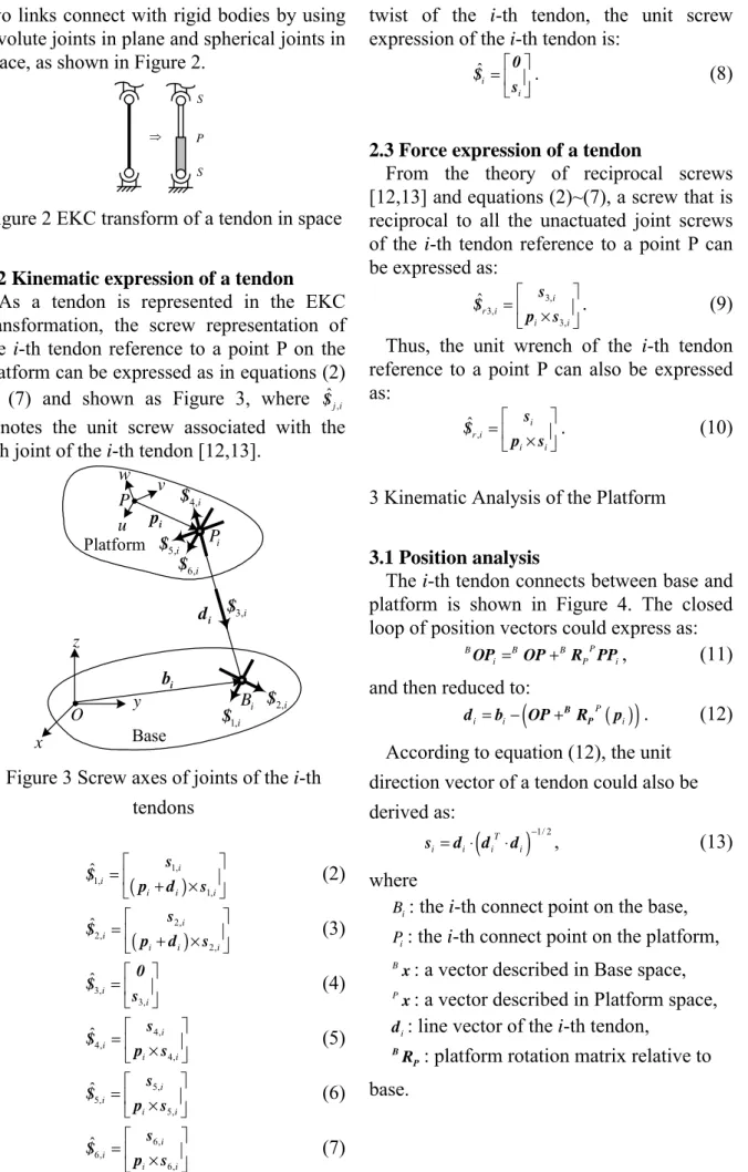
2.2 Kinematic expression of a tendon
As a tendon is represented in the EKC transformation, the screw representation of the i-th tendon reference to a point P on the platform can be expressed as in equations (2) to (7) and shown as Figure 3, where $ˆj i, denotes the unit screw associated with the
j-th joint of the i-th tendon [12,13].
x z u v w P i P i B i p i b i d 1,i $ y O 2,i $ 3,i $ 4,i $ 5,i $ 6,i $ Platform Base
Figure 3 Screw axes of joints of the i-th tendons ( 1,) 1, 1, ˆ i i i i i = + × s $ p d s (2) ( 2,) 2, 2, ˆ i i i i i = + × s $ p d s (3) 3, 3, ˆ i i = 0 $ s (4) 4, 4, 4, ˆ i i i i = × s $ p s (5) 5, 5, 5, ˆ i i i i = × s $ p s (6) 6, 6, 6, ˆ i i i i = × s $ p s (7)
Neglect the passive joints and consider the
twist of the i-th tendon, the unit screw expression of the i-th tendon is:
ˆ i i = 0 $ s . (8)
2.3 Force expression of a tendon
From the theory of reciprocal screws [12,13] and equations (2)~(7), a screw that is reciprocal to all the unactuated joint screws of the i-th tendon reference to a point P can be expressed as: 3, 3, 3, ˆ i r i i i = × s $ p s . (9)
Thus, the unit wrench of the i-th tendon reference to a point P can also be expressed as: , ˆ i r i i i = × s $ p s . (10)
3 Kinematic Analysis of the Platform
3.1 Position analysis
The i-th tendon connects between base and platform is shown in Figure 4. The closed loop of position vectors could express as:
P
B B B
i = + P i
OP OP R PP, (11)
and then reduced to:
( )
(
P)
i = −i + i B P d b OP R p . (12)According to equation (12), the unit direction vector of a tendon could also be derived as:
(
T)
1/ 2 i i i i − = ⋅ ⋅ s d d d , (13) where iB : the i-th connect point on the base,
i
P: the i-th connect point on the platform,
Bx: a vector described in Base space, Px: a vector described in Platform space,
i
d : line vector of the i-th tendon,
B P
R : platform rotation matrix relative to base.
x z u v w P i P i B i p i b i d y O
Figure 4 Position of base, platform and the
i-th tendons
3.2 Velocity analysis
The instantaneous twist of the platform can be expressed via the joints screws of the i-th tendon as: $ $ $ $ $ $ $ 6 , , 1 1, 2, 3, 4, 5, 6, 1, 2, 3, 4, 5, 6, j i P j i j P i i i i i i i i i i i i q d θ θ θ θ θ = = = = + + + + +
∑
& && & & & &
$ $ V $ $ $ $ $ $ ω , (14) where q&j i, is the velocity variable of the j-th joint of the i-th tendon, such as θ&j i, for revolute joint and d&j i, for prismatic joint.
The Jacobian of the i-th tendon, by applying the theory of reciprocal screws, could be shown as:
, ,
x i P = q i&i
J $ J q , (15)
and derived to:
$T 3, r i P =d&i
$ $ . (16)
When all tendons are considered, the final Jacobian is shown as:
x&= q& J x J q, (17) where $ $ $ ( ) ( ) ( ) ,1 1 1 1 ,2 2 2 2 , T T T r T T T r T T T r n n n n × × = = × M M M x p s s $ p s s $ J p s s $ , = q J I (n×n identity matrix), T x y z vpx vpy vpz ω ω ω = & x
the angular velocity and linear velocity of the platform, and 1 2 T n d d d
=& & &
& L
q
the linear velocity of tendons.
The relationship between base-platform space and actuator space can also be expressed as equation (18) by rearranging equation (17). x&= q& J' x' J q, (18) where ( ) ( ) ( ) 1 1 1 2 2 2 T T T T T T n n n × × = × M M x s p s s p s J' s p s , a (n×6) matrix, T px py pz x y z v v v ω ω ω = & x' .
4 Force Analysis of the Platform
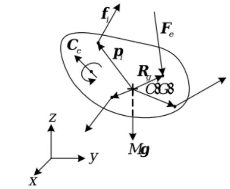
4.1 Dynamic equilibrium of the platform
In figure 5, a rigid body, the platform, is specified with its center of gravity, and exerted with n tensions, and gravity force. With respect to its C.G., these n tensions are transferred into a resultant external force and a resultant couple in space, and the dynamic equilibrium equation can be derived as:
1 1 n i e i n i i g g e g e i M M = = = − − × = + × − − ×
∑
∑
& f a g F p f H ω H C R F , (19) where:C.G. : center of gravity of the platform,
g: acceleration of gravity,
M : mass of the platform,
a: acceleration of the platform,
ω: angular velocity of the platform, i
f : tension force,
i
p: distance from C.G. to the tension
applying point, e
F : resultant external force,
g
R : distance from C.G. to the resultant
external force applying point, e
C : resultant couple,
g
e C e F Mg g R i p i f . . C G x y z
Figure 5 Forces and couple on the platform
Equation (19) could then be expressed in a matrix form as:
1 1 2 2 1 1 2 2 n n n n e g g e g e f f f M M × × × − − = + × − − × L L M & s s s p s p s p s a g F H ω H C R F , (20)
and presented in terms of tendon screws as:
$ $ $ 1 2 ,1 ,2 , r r r n n e g g e g e f f f M M − − = + × − − × L M & $ $ $ a g F H ω H C R F . (21)
4.2 Static equilibrium of the platform
From equation (20), as the dynamic terms are zero, the static equilibrium of the platform can be shown as:
$ $ $ 1 2 ,1 ,2 , r r r n n f f M f − = L M g $ $ $ 0 . (22)
Both equation (20) and (21) can be expressed as:
[ ]
ST 6×n{ }τ n×1={ }F 6 1× (23) where τ is the tendon force vector.4.3 Necessary condition of a full controlled TDP
The solution of tendon force, τ , in
equation (22) can be solved via pseudo inverse [14]:
(
)
+ + = Τ + − Τ Τ τ τ S F I S S K , (24)(
)
1 T T − + = Τ Τ Τ Τ S S S S , (25) where the(
− +)
Τ Τ τI S S K term is the null
space of tendon forces, τ.
Because the tensions of tendons are required to be maintained positive at all time in order to hold the position and orientation of the platform. The solutions of τ in equation (24) should be all greater than zero.
Thus, the components in the
(
− +)
Τ Τ τ
I S S K term in equation (24) must be all greater than zero in order to achieve the tendon positive tension condition. It is necessary to have an all-positive null vector combination, in the case, n>6. For this reason, a TDP is said to be fully controlled only if the number of tendons is greater then the mobility of the platform, which means: n>6 in equation (23). In the case of n≤6, the motion of platform is not fully controlled, yet still partially workable in some area and some direction.
Under the fully controlled condition, the solution of platform kinematics, x&, in equation (17) could also be solved via pseudo inverse:
(
)
+ + = + − & x & x x x x J q I J J K , (26)(
T)
−1 + = x x x x J J J J . (27) where the(
− +)
x x xI J' J' K term is the null space of tendon velocities, x&. The solution yields infinite solutions of x& yet the null space is not necessarily all-positive.
5 Singularity Analysis
In some particular positions and orientations of a platform, the Jacobian matrix may lose its full rank and results in the singular conditions. Under these conditions, the platform may gain one or more degree of freedom within its workspace, and therefore loses its stiffness completely, which means the platform is uncontrollable. Another critical factor is that the tensions of the tendons also affect the stiffness and configuration of the platform. Therefore, the
kinematic singularity, kinetic singularity and tension condition should be discussed in details in order to determine the controllable workspace of the TDPs.
5.1 Kinematic singularity analysis
The platform can possess infinitesimal motion in some direction while all the tendon displacements are completely unchanged when the direct kinematic singularity occurs. Under this condition, the platform may gain one or more degree of freedom, but cannot resist forces or moments in certain directions. It happens when the Jacobian matrix loses its rank.
For a full controlled TDP, the matrix Jx is a n×6 matrix in equation (17), and n>6;
therefore, the maximum rank of Jx is 6. In the case that rank[ ] 6Jx < , it is said Jx loses its rank and results in a kinematic singularity.
5.2 Kinetic singularity analysis
All the tensions of the tendons are undetermined and the platform is uncontrollable when the kinematic singularity occurs. It happens when the matrix ST in equation (23) loses its rank.
For a full controlled TDP, the matrix ST is
a 6 n× matrix, and the maximum rank of
T
S is 6 since n>6 . In the case that
[ ]
rank ST <6, it is said that ST loses its rank
and results in a kinetic singularity.
Comparing equations (18) and (23), the relationship between J'x and ST is:
T
x T
J' = S . (28)
It is clear that the kinematic singularity and kinetic singular will happen at the same time. Thus, only one of the rank of matrix J'x or
T
S is needed to be check to determine the singularity.
Another important issue in the force analysis is that the null space of τ in equation (24) should be positive all time to consist with the tension condition of tendons. If some components in τ are negative, it means the forces on the tendons are not tensive force and these tendons are loosed. The platform will be not fully controlled even the rank of ST is still 6.
5.3 TDP controllable workspace
The controllable workspace of TDP can be defined as the set of postures where forces and torques on the platform can be controlled under the following conditions:
(i) all tendon forces must be positive;
(ii) the platform must not run into
singularities.
Therefore, the controllable workspace of TDP can be determined by checking:
(i) rank
[ ]
ST =6 (or rank[ ] 6Jx = );(ii)
(
− +)
T T
I S S K > 0.
These matrices are all established based on screw axes and consistent with kinematic and force analysis.
6 Example
Referring to figure 1, it’s a spatial eight-tendon platform, and used as an example to illustrate the method. In the analysis, the first step of this unified approach is to establish the screw representations of tendons via inverse position analysis to get si and pi which are expressed in base space. In this procedure, we needs to know the position of the center of gravity of the platform,po, and the rotation matrix of platform relative to the base, B
P
R . After the inverse position analysis, the Jacobian of the platform can be derived directly and shown as in equation (29):
$ $ $ ,1 ,2 ,8 T r T r T r = M x $ $ J $ , (29) where ( ) , ˆ T T T r i i i i = × $ p s s . (30)
And the kinematic relationship of tendons and platform can established easily as in equations (31) and (32):
& x&
(
)
+ +
= + −
& x & x x x
x J q I J J K , (32)
When the platform is under the static equilibrium condition, there is no dynamic term, and the force relationship among tendons and platform can be derived as:
[ ]
{ }=−M ={ } τ T S g S F 0 , (33)If the dynamic terms are considered, the dynamic equilibrium can be shown as:
[ ]
{ } e { } g g e g e M −M − = + × − − × = & τ ω T D a g F S F H H C R F , (34) and brief expressed as:[ ]
ST { } { }τ = F (35) where[ ]
$ $ $ ,1 ,2 ,8 r r r = L T S $ $ $ , (36) $ ,1 i r i i = × s $ p s , (37) { } { 1 2 8} T f f f = L τ . (38)Thus, the kinetic relationship of tendons and platform can established rapidly as in equations (39) and (40): τ T F = S (39)
(
)
+ + = Τ + − Τ Τ τ τ S F I S S K (40)Because the platform is actuated by all eight tendons, the platform can be a fully controlled TDP. This platform can perform six degree-of-freedom motions and resist external forces and couples, or be maintained in static equilibrium under the following conditions:
(i) matrixSTis full rank (or matrixJxis full
rank);
(ii) fi >0 in { }τ .
From the example via the unified approach, the kinematic and force analysis, and the controllable workspace determination, therefore, are indeed more efficient and simplified.
7 Conclusions
In this study, the tension and the posture of the tendons can be expressed in the form of screw axes to represent the corresponding wrenches and twists directly and properly.
And then, the kinematic and force analysis model of tendons and platforms can be established intuitively. Through the example, it is believed that the unified approach based on the screw theory is indeed straightforward and efficient.
8 Reference
1. W.B. Garrett, “Suspension System for Supporting and Conveying Equipment, such as a Camera”, United States Patent, No. 4625938, 1986.
2. Roger Bostelman, James Albus, Nicholas Dagalakis, Adam Jacoff, “Application of The NIST ROBOCRANE,” Robotics and Manufacturing, Vol. 5, 1994.
3. P. D. Campbell, P. L. Swaim, and C. J. Thompson, “Charlotte Robot Technology for Space and Terrestrial Applications,” SAE Technical Series paper 951520, 1993.
4. Duan, B. Y, “A new design project of the line feed structure for large spherical radio telescope and its nonlinear dynamic analysis”, Mechanism 1, 1999.
5. Y. X. Su, B. Y. Duan, R. D. Nan, B. Peng, “Development of a large parallel-cable manipulator for the feed-supporting system of a next-generation large radio telescope”, Journal of Robotic System 18(11), 2001. 6. Robert L. Williams II, “Cable-Suspended
Haptic Interface”, International Journal of Virtual Reality 1, Vol. 3, No. 3, pp. 13-21, 1998
7. S. Kawamura, W. Choe, S. Tanaka, S. R. Pandian, “Development of an Ultrahigh Speed Robot FALCON using Wire Driven System,” IEEE International Conference on Robotics and Automation, 1995.
8. Tetsuya Morizono, Kazuhiro Kurahashi, Sadao Kawamura, ”Realization of a Virtual Sports Training System with Parallel Wire Mechanism”, Proceedings of the 1997 IEEE International Conference on Robotics and Automation, Albuquerque, New Mexico, April 1997. 9. Aiguo Ming, Toshiro Higuchi, “Study on
Mechanism Using Wires (Part 1),” Int. J. Japan Soc. Prec. Eng., Vol. 28, No. 2 (June 1994).
10. Aiguo Ming, Toshiro Higuchi, “Study on Multiple Degree-of-Freedom Positioning Mechanism Using Wires (Part 2),” Int. J. Japan Soc. Prec. Eng., Vol. 28, No. 3 (June 1994).
11. Aiguo Ming, Makoto Kajitani, Toshiro Higuchi, “On the Design of Wire Parallel Mechanism,” Int. J. Japan Soc. Prec. Eng., Vol. 29, No.4 (June 1995).
12. Lung-Wen Tsai, ”Robot Analysis---- the Mechanics of Serial and Parallel Manipulators”, John Wiley and Sons, Inc., 1999.
13. Yuan, M. S. C., Freudenstein, F., and Woo, L. S., “Kinematic Analysis of Spatial Mechanisms by Means of Screw Coordinates, Part 1: Screw Coordinates,” ASME J. Eng. Ind., Vol. 93, Ser. B, No. 1, pp. 61-66, 1971.
14. Edward M. Landesman, Magnus R. Hestenes,” Linear Algebra for Mathematics, Science, and Engineering”, Prentice Hall, 1992. 四、PART II 軌跡規劃與策略 此部分研究提出腱驅動平台之軌跡規 劃策略,發展腱驅動平台沿特定軌跡運動 之計算邏輯與方法,並以各腱速度平方和 為目標函數對軌跡規劃進行最佳化。首先 針對腱驅動平台之逆向運動學與速度分析 做探討;其次將平台運動軌跡分為路徑與 速度規劃,討論直線、圓弧和三次曲線段 合成路徑,同時提出修正梯形速度曲線改 善梯形速度曲線加速度不連續之缺點;接 下來發展出腱驅動平台的軌跡規劃策略, 並藉由數值模擬探討及驗證策略之可行 性;最後利用平台方位角的變化對軌跡規 劃進行最佳化,並且利用數值範例驗證最 佳化之成效。此部分研究結果可提供腱驅 動平台運動命令產生所需原理、方法和步 驟之參考。 1 背景與緣由 並聯式機構在定位平台與工具機已有 廣泛之應用,與串聯式機器人相較,並聯 式驅動機器人具有簡單的逆向運動學、較 高剛性、較高負載能力以及高速運動等優 點[1]。此部分研究所討論之腱驅動平台 (Tendon-Driven Platform, TDP)即是以腱做 為傳動線的並聯式機構,藉由調整腱的長 度進行對工作平台之操控,於平面具有三 個自由度,空間中具有六個自由度,其中 腱泛指僅能負載拉力而無法承受壓力及力 矩的物體,如:線(wire)、細繩(string)、纜 線(cable)等;由於此限制使得n條腱並無法 操控平台n個自由度,Kawamura [2]說明了 至少需要n+1條腱才能操控n個自由度,因 此腱驅動平台所需的最少腱數,在平面需 四條腱,空間中則需七條腱。腱驅動平台 除了有並聯式機構的優點之外,與傳統並 聯式機構相較下還有架設容易、機構整體 質量小的優點;同時腱驅動平台具有撓性 元件本身之優點:長距離的能量傳遞、質 量輕、簡單的機械設計等。 腱驅動平台的運動可分為平台的運動 和腱的運動,平台的運動軌跡常是平台所 必須執行的任務,腱的運動軌跡則是實際 控制的部分,所以腱的運動軌跡必須符合 物理上的限制或是其他的要求,這使得軌 跡規劃(trajectory planning)成為在操作平 台之前的重要工作。 目前對於腱驅動平台的研究包括有原 型機的試驗、運動學、靜力學、各腱張力 的計算、線型態配置、奇異點、靜態與動 態工作空間、腱張力的調配和多餘度的討 論等,關於腱驅動平台軌跡規劃則少有完 整討論,僅有Ming和Higuchi[3]提出的直線 軌跡規劃法,以及邱[4]所提出的腱驅動平 台在直線路徑下的速度最佳化之運動軌跡 規劃,可作為此部分研究運動規劃之參 考。關於並聯式平台軌跡規劃相關文獻則 有Nguyen等人[5]發展之以Stewart平台機 構為操作器(manipulator)的軌跡規劃法,使 操作器遵循一直線運動;Huynh和Arai [6] 提出並聯式操作器在工作空間中極限速度 分析的圖解法及運算法則,使得並聯式操 作器的設計者可以迅速地了解操作器的極 限速度,同時提出操作器的速度允許區域
的大小可作為在運動學下性能測量的標 準;Huynh等人[7]則以並聯式操作器極限 速度理論為基礎,提出固定式線性驅動並 聯式操作器的直線軌跡最佳速度控制。除 了簡單的直線運動之外,為了使平台能夠 平滑地經過某些特定點,需要平滑曲線將 這些點連接。平滑曲線的產生方式在電腦 輔助繪圖已有許多的研究成果,如三次曲 線(cubic splines)、Bézier曲線、B-spline曲 線[8]等。由於三次曲線為保證各曲線段在 連接點處達到二階導函數連續的最低次數 曲線,為了簡化分析此部分研究將以三次 曲線作為主要討論的運動路徑。由前人研 究可知,目前未有針對腱驅動平台軌跡規 劃做統整性的分析與討論,雖然已有許多 控制系統提出[9][10][11],但多為即時搖桿 控制或是點到點控制,對於運動命令的產 生卻少有討論,因此此部分研究將針對腱 驅動平台的軌跡規劃進行探討,藉由直接 對平台進行軌跡規劃,產生符合物理限制 的各腱運動軌跡,以作為腱驅動平台運動 控制系統的參考輸入,並提出腱驅動平台 之軌跡規劃策略。除了做為實際操作時的 參考命令之外,還可以於平台運動之前, 先行了解各驅動器之運動,更加充分掌握 整個系統的特性。此外提出以各腱速度平 方和為目標函數,對於軌跡規劃進行最佳 化之方法,並以數值模擬驗證最佳化之成 效。 2 運動學與力學分析 首 先 對 腱 驅 動 平 台 的 逆 向 運 動 學 和 Jacobian矩陣進行推導與分析,得到平台位 置姿態與腱長之間的關係,以及平台速度 與各腱速度之關係,並說明腱驅動平台順 向奇異點發生之時機;接下來討論腱驅動 平台在運動學和力學上的限制:由腱速度 之限制推得平台速度的限制範圍,由腱張 力須為正的限制來定義腱驅動平台的可工 作點。 2-1. 逆向運動學分析 如圖1所示為一空間八腱平台示意圖。 平台坐標系統P與基座坐標系統B之間的 轉換,可以由平台坐標原點P0於基座坐標 之位置向量與旋轉矩陣B P R 來描述,使用 Roll-Pitch-Yaw的角度表示法來描述平台 相對基座坐標的姿態(orientation):若平台 坐標原點與基座坐標原點重合,平台坐標 對基座坐標的x軸旋轉ψ,再對y軸旋轉θ, 最後對z軸旋轉φ角度,這些角度稱為方位 角,三個對於基座坐標連續的旋轉可得旋 轉矩陣B P R 。n條腱的基座接點於基座坐標 的位置向量為Bi (i=1, 2, , )K n ,平台接點於 平台坐標的位置向量為Pi (i=1, 2, , )K n ,則 i P 於 基 座 坐 標 的 位 置 向 量BPi 為Pi 前 乘 B P R 。腱驅動平台的逆向運動學為給定平 台坐標原點的位置向量B 0 P 和平台坐標相 對基座坐標的旋轉矩陣B P R 後,得到對應 之各腱腱長。 1 B 2 B 3 B 0 B x y z 0 P x y z 1 P 2 P 3 P 圖1 腱驅動平台示意圖 由圖2-1知關於第一條腱的向量迴路方 程式可寫成為式(1),將式(1)以基座坐標位 置向量通式改寫,得到第i條腱的向量迴路 方程式如式(2)所示,其中B i L 為腱向量P Buuuuvi i 方向由平台接點指向基座接點。 1 1 1 0 0 0 0 1 0 P B +B B +B P +P P= uuuuv uuuuuv uuuuuv uuuuv
(1) B B B 0 0 i− i + + i = L B P P (2) 將式(2)移項可得腱向量B i L ,所以第i 條腱長度Li的平方值可以由該腱之腱向量 與自己本身內積而得。因此給定平台位置 姿態後,第i條腱長度可寫成 B B B B 1/ 2 0 0 ([ ] [T ]) i i i i i L = B − P − P B − P − P (3) 又將式(3)改寫成式(4),其中L為各腱長 所組成之腱長向量,
[
]
T ψ θ φ = Φ 為平台 方位角向量,式(4)表示各腱長為平台位置 姿態之函數,即是腱驅動平台位置控制的 主要方程式。 B 0 ( , ) f = L P Φ (4)2-2. Jacobian矩陣分析 對腱驅動平台而言,Jacobian矩陣表示 出平台速度到腱速度的對應,當平台的位 置與姿態改變時,Jacobian矩陣中的各元素 也隨之改變。Jacobian矩陣可利用各腱平台 接點向量B B 0+ i P P對時間微分推得。微分後 可得平台接點Pi於基座坐標的速度 i P V 0 0 B i P = P + P × i V V Ω P (5) 其中 0 0 0 0 x y z T P =vP vP vP V 為平台坐標原點 於 基 座 坐 標 的 線 速 度 , 0 0x 0y 0z T P =ωP ωP ωP Ω 為平台坐標於基座坐 標的角速度。第i條腱之速度 i L V 為式(5)中平 台接點速度 i P V 在第 i 條腱單位向量li上 投影即 V l i i L P i V = ⋅ B B (l L ) L i i i = (6) 式(5)代入式(6)得到式(7),再將式(7)寫成矩 陣 形 式 , 對 於 n 條 腱 速 度 向 量 1 2 n T L=VL VL VL V L 可寫為式(8),其中J 為腱驅動平台Jacobian矩陣。 0 0 0 0 0 0 B B B ( ) ( ) ( ) i L P P i i P i P i i i P i i P V = + × ⋅ = ⋅ + × ⋅ = ⋅ + × ⋅ V P l V l P l l V P l Ω Ω Ω (7) 0 0 0 0 B 1 1 1 B 2 2 2 B ( ) ( ) ( ) T T T T P P L P P T T n n n × × = = × l P l V V l P l V J l P l M M Ω Ω (8) 對於平面腱驅動平台,若Rm為m維實數 空 間 , 則 3, 0 2, 0 1 i∈R P ∈R P ∈R l V Ω , 故 3 n R × ∈ J ; 對 於 空 間 平 台 , 0 0 6, 3, 3 i∈R P ∈R P ∈R l V Ω , 故J∈Rn×6。 因 此 Jacobian矩陣在平面時為滿秩數(rank)為 3 , 在 空 間 中 滿 秩 數 為 6 。 以 向 量 B 0 x= P ΦT表示平台的位置與姿態,L為 各腱長度所組成之腱長向量,式(8)可以改 寫為式(9),其中「.」代表對時間的一次 微分,式(9)為腱驅動平台速度控制主要方 程式。 = L& J x& (9) 當Jacobian矩陣失去秩數的時候,平台此時 的位置與姿態即是腱驅動平台之順向運動
學 奇 異 點 (direct kinematic singular
point)[12],由式(9)可知,若腱速度L&為0 時,由於Jacobian矩陣失去秩數,平台速度 x&會有0以外的解,也就是腱長不產生變 化,平台仍能產生某自由度的運動。腱驅 動平台常見的順向奇異點位置會發生在, 各腱於基座坐標接點所形成之多邊形與對 應之平台接點所形成多邊形相似時,平台 應避免選擇上述之線型態,否則平台可能 因無法承受某些方向之作用力或作用力 矩,使得平台失去控制。 2-3. 平台極限速度 當並聯式平台在運動時,由於各驅動器 的速度受到限制,平台的速度也受到了限 制,這個限制在平台的速度控制或是軌跡 的產生扮演相當重要的角色,藉由了解此 限制關係,可使得平台在執行任務時可以 盡量發揮驅動器的性能[6]。對於腱驅動平 台而言,腱的極限速度Vlim是決定平台極限 速度的主要因素,腱的極限速度則是由驅 動馬達的極限速度和捲線軸的直徑尺寸所 決定,用式(10)表示腱極限速度與腱速度的 關係,由式(9)可以得到腱速度與平台速度 的線性關係,所以當給定了平台的位置及 姿態,平台的速度必須符合式(11)的限制, 式中
[ ]
Ji 代表Jacobian矩陣的第i列。 lim ( 1, 2, , ) i L V ≤V i= K n (10)[ ]
0 0 lim lim T i P P V V − ≤ J V Ω ≤ (i=1, 2, , )K n (11) 式(11)中的平台速度 0 0 T P P V Ω 形成一 向 量 空 間 (vector space) , 而[ ]
0 0 lim T i P P = ±V J V Ω 則 形 成2n 個 超 平 面 (hyper-plane),每個超平面將平台速度向量 空間分割成等於零、大於零以及小於零三 個區間,每個限制不等式決定一個超平面 的區間,而所有的超平面區間的交集就是 平台速度允許區域,區域的邊界即是平台 的極限速度。以平面四腱腱驅動平台為 例,給定平台位置姿態[
]
T x y φ = x ,若平 台姿態維持不變時,即 0 0 z P ω = ,則平台速 度為 0 0 0 x y T P P v v = x& ,可得到八組限制不 等式,如式(12)所示,此八組限制不等式在 以vP0 x為橫軸、vP0 y 為縱軸的二維平面上交 集出平台速度允許區域。 0 0 lim i1 Px i2 Py lim V J v J v V − ≤ ⋅ + ⋅ ≤ ( 1, 2,3, 4)i= (12)2-4. 可工作點 由於撓性元件只能傳遞拉力,無法承受 壓力,亦無法承受彎曲力矩,所以進行腱 驅動平台的控制時,首先必須檢驗腱元件 是否仍是緊繃的狀態。腱驅動平台所需的 最少腱數,在平面中需四條腱,空間中需 七條腱,平面可提供三個力學平衡方程 式,空間則可提供六個方程式,腱張力未 知數較可提供的方程式為多,所以是靜不 定系統,具有無限多組解,但只有大於零 之解,才符合撓性元件的限制。以下藉由 腱驅動平台力學方程式的推導,來說明腱 驅動平台可工作點之定義。首先說明楊 [13]所進行的腱驅動平台力學方程式推 導:由虛功原理得到式(13),其中τ為各腱 張力所構成之向量,F為平台於平台坐標 原點之輸出力與輸出力矩構成之向量,δx 為平台位置姿態變化量,δL為腱長度變化 量。由式(9)可知,腱長度變化量與平台位 置姿態變化量具有式(14)的關係,將式(14) 代入式(13),並將等號兩邊的δx消去且轉 置後,可得式(15)的關係式。 Tδ = Tδ F x τ L (13) δL=J xδ (14) T = F J τ (15) 式(15)表示腱張力與輸出力、輸出力矩 的關係,其中JT為轉置Jacobian矩陣,平面 時 T 3n R× ∈ J 空間時JT∈R6×n,n表腱數。由於 T J 非 方 陣 , 需 使 用 文 獻[14] 所 提 之 pseudoinverse,得到腱張力τ通解 # ( # ) =A F+ −I A A z τ (16) 其中 = T A J ,A#為A的pseudoinverse,在平 面時 # n 3 R × ∈ A ,空間中A#∈Rn×6,z∈Rn為n 維 的 任 意 向 量 , 當JT 未 失 去 秩 數 時 , # = T( T)−1 A A AA 。式(16)可進一步表示成式 (17),其中右式的第一項為式(15)的特解, 第二項h則為式(15)的齊性解,即 T J 的零空 間(null space),是 ( )T n−rank J 個零向量(null vector)的線性組合,所以對於平面四腱腱 驅動平台且JT未失去秩數時,h由一個零向 量組成,對於平面五腱平台且 T J 未失去秩 數時,h由兩個零向量線性組合。若為平面 四 腱 腱 驅 動 平 台 時 , 腱 張 力 為
[
1 2 3 4]
T τ τ τ τ = τ ,式(17)可寫成式(18), 其中[
1]
T a b c 為零向量,c1為任意實數。 # =A F+h τ (17)[
]
#[
]
1 2 3 4 A F 1 1 T T c a b c τ τ τ τ = + (18) 當輸出力及力矩F為0時,式(17)簡化成 靜力平衡方程式,腱張力τ等於零空間h, 故零空間h各元素值必須皆大於零才能符 合腱張力的限制。又當平台靜止時受到外 力或外力矩作用於其上,各腱所傳遞的拉 力必須能輸出等量且反向之力或力矩,以 抵抗外力或外力矩在此位置達成靜力平 衡,此時式(17)中 # A F為一特定值,若零空 間h中的各零向量藉由調配能夠使得零空 間h各元素值皆大於零,表示不論F為何值 各腱張力τ皆能夠維持正值。若當平台在 運動時,是受到腱張力作用其上而產生運 動,因此各腱也需輸出力或力矩以提供平 台運動所需,和靜止時受外力或外力矩作 用的情況相同。因此在此部分研究中將JT 未失去秩數且能保證其零空間h中的各元 素值皆大於零,此時平台的位置與姿態定 義為可工作點。平台的運動軌跡都必須符 合可工作點的定義,才是安全的運動軌跡。 3 平台之運動軌跡 腱驅動平台運動時受到各腱並聯連接 的限制,各腱之驅動器無法獨立運動,彼 此之間為相依關係,因此較適合於任務空 間進行軌跡規劃,平台的運動軌跡即是指 平台在任務空間的運動軌跡,此軌跡為決 定平台位置與姿態的時間函數x(t),使得平 台在特定時間條件下,沿著特定路徑由起 點運動至終點。軌跡可區分為幾何路徑和 速度規則兩部分,若將路徑函數以路徑長 為參數表示時,速度規則即是規劃此參數 隨時間的變化。在空間中起點為Pb終點為 Pe的一直線,其參數表示法如式(19)所示, 0 s= 時代表起點Pb,s= Pe−Pb 時則代表終 點Pe。 ( ) ( ) P P P P P P b e b e b s s = + − − (19) 定義圓路徑時,需給定垂直於圓平面之 圓心軸單位向量Γ,圓心的位置向量c,以 及 圓 的 起 點 的 位 置 向 量Pb , 圓 半 徑 為 Pb c ρ = − 。在圓上定義一新坐標系統C, 其原點與圓心重合,其x軸由圓心指向起點 Pb,z軸沿著圓心軸Γ,y軸則由右手定則所 決定,此時圓上各點在坐標系統C可以容易地以參數s表示,如式(20)所示。圓上的 點在基座坐標的參數表示法可藉由坐標轉 換得到,如式(21)所示,其中B C R 為坐標C 相對於基座坐標B的旋轉矩陣,由坐標C的 x, y, z軸的單位向量所組成[15]。 C cos( / ) ( ) sin( / ) 0 P s s s ρ ρ ρ ρ = (20) B C C ( ) ( ) P s = +c R P s (21) 平台的運動除了基本的直線路徑或圓 弧路徑或兩者的複合路徑外,常常需要通 過有限個已知的特定點,為了能夠平滑的 通過各點,此部分研究以三次曲線段將各 點連接,首先將三次曲線段以u為參數來表 示 如 式 (22) 所 示 , 其 中
[
]
( ) ( ) ( ) ( ) P u = x u y u z u 為 三 次 曲 線 段 上 任 一 點 的 位 置 向 量 , 四 個 係 數 向 量 Ci ( 1, 2,3, 4 i= )必 須 要 由 四 個 邊 界 條 件 來 求 得 , u1和 u2為三次曲線段兩端點的參數 值,u1和u2的選擇會影響曲線的平滑度, 為了簡化計算並且維持曲線平滑度,令u1 為0,u2為 P2−P1 。 4 1 1 2 1 ( ) P Ci i i u u− u u u = =∑
≤ ≤ (22) 可推得第k個曲線段的各項係數如式 (23)所示,其中C1k代表第k個曲線段的C1係 數 1 2 2 2 1 1 1 1 3 1 4 1 3 2 3 2 1 1 1 1 1 0 0 0 0 1 0 0 3 2 3 1 2 1 2 1 C P C P C P C P k k k k k k k k k k k k k k k k u u u u u u u u + + + + + + + + + + ′ =− − − ′ − (23) 若將三次曲線段以邊界條件來表示,可 推得第k個三次曲線段上的各點成為以λ 為 參 數 之 函 數 , 即[
]
( ) ( ) ( ) ( ) Pk λ = xλ y λ z λ ,如式(24)所示,λ 代表權重介於0與1之間,較參數u更能夠直 觀地了解各點於三次曲線段上所在之位 置。 [ 1 2 3 4 ] 1 1 ( ) ( ) ( ) ( ) ( ) P P P P P k k k k k k k k k F F F F λ λ λ λ λ + + ′ = ′ (24) 上式中 1 , 0 1 k u u λ λ + = ≤ ≤ 3 2 1 2 2 1 3 2 3 2 4 1 ( ) 2 3 1 ( ) ( 2 1) ( ) 2 3 ( ) ( ) k k k k k k F F u F F u λ λ λ λ λ λ λ λ λ λ λ λ λ λ + + = − + = − + = − + = − 為了保證在各接點處之二次微分值連 續,邊界條件會有所限制,由此限制可推 得接點處的切線向量必須符合式(25)之關 係。所以當給定端點之切線向量後便可求 得所有接點切線向量,進而求得所有點。 接下來將P( )λ 改以路徑長為參數表示,由 於Pk( )λ 為三次多項函數,所以其一次微分 於區間[0,1]為連續,第k個三次曲線段的曲 線長sk( )λ 可由式(26)求得,由式(26)可知路 徑長s與λ之關係為非線性方程式,當已知 s時,需藉由數值方法(如牛頓法)求解對 應之λ值後,再代入式(24)得到平台所在之 位置向量,如此可將路徑長s對應至參數 λ。 2 1 2 1 1 1 2 2 1 2 1 2 1 1 2 2( ) 3 [ ( ) ( )] 1 2 P P P P P P P k k k k k k k k k k k k k k k u u u u u u u u k n + + + + + + + + + + + + + ′+ + ′ + ′ = − + − ≤ ≤ − (25) 2 2 2 0 ( ) ( ( )) ( ( )) ( ( )) k s λ =∫
λ x′ξ + y′ξ + z′ξ dξ (26) 欲得各路徑上某點P之速度和加速度 時,可將各路徑函數P s( )對時間做一次微 分和二次微分得到。 接著規劃路徑長隨時間的變化,即平台 特定點之線速度規劃,一般平台的運動通 常在起點和終點是靜止的,而且希望能以 較短時間運動,所以需要由靜止加速至最 高速度,維持最高速度一段時間,再經過 減速達到靜止,在符合前述的要求下,最 常被使用到的是梯形曲線,但有速度變化 不平滑的缺點,因此此部分研究提出一修 正梯形曲線,在與梯形曲線相同的輸入條 件下,改善梯形曲線不平滑的缺點。利用 路徑長為擺線曲線(cycloid curve)時,其加 速度曲線為一連續函數的特性,將梯形速 度曲線作一修正,如圖2所示,當給定和梯 形速度曲線相同的初始條件:加速時間 a i t −t 、等速度s&a和行進的路徑長sf −si時, 可以得到修正梯形速度曲線所需要的各項參數值,如式(27)所示,其中R,ϕ ϕa, d 為擺 線曲線所必須使用到的參數。 圖2 修正梯形速度曲線 , , 2 ( ), ( 2 ) , 2 f a i d i f d a i a a a i d d f a i a i a i a d a i a a i s t t t t t t t t R s s t t t t t t t t t t t s s s t t π π π ϕ ϕ π ϕ ϕ − = + = + − = = − = − + − − − = = = + − & &
& & &
(27) 於是可以得到修正梯形速度曲線的路 徑長對時間的函數、速度函數以及加速度 的函數,如式(28)、式(29)和式(30)所示。 ( sin ) ( ) ( ) ( ) ( sin ) i a a i a a a a a d i a d a d d d f s R t t t s t s s t t t t t s s t t R t t t ϕ ϕ ϕ ϕ + − ≤ ≤ = + − < ≤ + − + − < ≤ & & (28) (1 cos ) ( ) (1 cos ) a a i a a a d d d d f R t t t s t s t t t R t t t ϕ ϕ ϕ ϕ − ≤ ≤ = < ≤ − < ≤ & & & & (29) 2 2 (sin ) ( ) 0 (sin ) a a i a a d d d d f R t t t s t t t t R t t t ϕ ϕ ϕ ϕ ≤ ≤ = < ≤ < ≤ & && & (30) 平台運動時除了位置的改變外,還會有 姿態的改變,平台姿態的變換即是平台坐 標系統相對於基座坐標原點發生轉動,平 台 姿 態 由 對 基 座 三 個 坐 標 軸 的 方 位 角
[
]
T ψ θ φ Φ = 所描述,藉由規劃Φ( )t 的軌跡 即可對平台姿態作規劃,可利用前述位置 軌跡規劃之方法進行規劃。平台角速度即 是Φ( )t 對時間的微分,如式(31)所示。 0 0x 0y 0z T T P P P P d d d dt dt dt ψ θ φ ω ω ω Ω = = (31) 得到平台位置軌跡和姿態軌跡後,即完 成對於平台運動軌跡的完整描述,這些資 訊是在進行腱驅動平台軌跡規劃時所必須 使用到的,不完整的平台運動軌跡描述, 無法得到正確的各腱運動軌跡。 4 軌跡規劃策略 根據腱驅動平台位置控制和速度控制 方程式,以及平台極限速度和可工作點的 限制,配合平台運動軌跡之產生,進行腱 驅動平台之軌跡規劃。以下將對腱驅動平 台軌跡規劃之流程作詳細說明。 為了描述平台的運動,通常會指定一特 定點,把平台運動簡化為該特定點的運 動,此特定點常是執行任務的點,首先假 設平台特定點的位置路徑是任務的主要要 求,平台姿態則無要求,平台坐標原點設 定於平台特定點,基座坐標原點設定於某 一腱於基座之接點,基座坐標x軸平行於基 座坐標原點與鄰近一基座接點的連線,當 平台坐標x軸對於基座坐標各軸之方位角 皆為0時,稱平台姿態沒有改變。接著是平 台特定點運動路徑的產生,在此時平台沒 有改變姿態,將路徑以路徑長為參數表 示,得到位置路徑後,檢驗是否有奇異點 存在於路徑上,即檢查Jacobian矩陣是否失 去秩數,若有奇異點存在則需重新設定各 接點位置,如果沒有則進行可工作點檢 查,檢驗轉置Jacobian矩陣的零空間中各元 素是否皆大於零,路徑若通過不可工作 點,同樣必須修正接點位置(調整接點位 置即是改變基座與平台的幾何形狀及尺 寸),使得路徑上皆無不可工作點。符合奇 異點與可工作點的檢查之後,接下來進行 平台極限速度分析,了解平台於該運動路 徑上所能到達的極限速度,做為規劃位置 速度曲線之參考,以梯形速度曲線為例即 是決定其等速度值的參考。在決定位置速 度曲線之後即完成對位置軌跡的規劃。若 平台在軌跡上有姿態的要求,則必須進行 平台姿態軌跡規劃,首先是姿態路徑的產 生,配合位置路徑,檢查路徑上是否有奇 異點或不可工作點,若有則需產生一新姿 態路徑,接著在已知線速度與平台姿態 下,根據平台極速分析,求得在此姿態路 徑與位置軌跡下平台的極限角速度,在此 角速度的限制之下,規劃姿態速度曲線。 得到位置軌跡及姿態軌跡後,即完成對平 台運動的描述。此時已知平台位置姿態, 藉由逆向運動學可得各腱腱長隨時間變化 的曲線;已知平台線速度與角速度,透過 Jacobian矩陣可得各腱的速度曲線,這兩個曲線即是控制平台運動的參考命令,根據 這些資料來驅動各腱之馬達。軌跡規劃的 流程圖如圖3所示。 圖3 軌跡規劃策略流程圖 5 軌跡規劃之最佳化 腱驅動平台在平面擁有3個自由度,在 空間中有6個自由度,當平台沿著特定位置 軌跡運動時,可以利用一個方位角的變 化,對於平台運動軌跡進行最佳化,使得 各腱有較佳的表現,如降低各腱速度值 等。以平面腱驅動平台為例,在給定平台 的位置軌跡下,藉由平台對z軸旋轉自由度 的變化所求得之最佳平台角度軌跡,使得 各腱速度平方和最小,也就是平台在相同 的路徑與線速度下,藉由改變平台的姿 態,使腱長隨時間變化的曲線更為平滑, 降低各腱速度值,達到減少馬達轉動動能 的目的。 5-1. 設計變數與目標函數 此部分研究所討論的最佳化問題為:在 給定平台的位置軌跡和起點終點姿態之 下,利用平台一個方位角的變化,求得最 佳平台角度軌跡,使各腱速度平方和最 小。由於各腱速度是由平台位置軌跡和姿 態軌跡所決定,姿態軌跡目前還未知,為 了得到姿態軌跡,此部分研究採用的方法 為:在已知的平台位置軌跡的起點與終點 之 間 等 分 成 m+1 段 , 得 到 m 個 節 點 Pj (j=1, 2, , )K m ,平台於這m+2個點(m個 節點、起點P0和終點Pm+1)的方位角配合 該點的時間敘述,以三次曲線段連接之後 可以得到連續的角度曲線和角速度曲線即 平台的姿態軌跡。在已知位置軌跡下,由 於腱速度 i L V 為平台方位角φ和角速度φ&的 函數,不同的方位角會得到不同的姿態軌 跡,配合位置軌跡,可得不同的腱速度曲 線,因此設計變數就是平台於各節點的方 位角φj,目標函數設定為平台於各相鄰兩 節點之中間點的腱速度平方和,對於m個 節點則會有m+1個中間點,假設腱驅動平 台有n條腱,平台於第k個中間點時第i條腱 速度以 ( ) i k L V 表示(k=1, 2, ,K m+1),目標函數 可寫成為式(32)。利用最佳化方法尋找出平 台在這有限個節點之方位角,使得目標函 數有最小值。
( )
( )[
]
1 2 1 2 1 1 ( ) , i k n m T L m i k f Φ V Φ φ φ φ + = = =∑∑
= L (32) 由於腱張力須大於零的限制,設計變數 j φ 亦受到限制,φjmin和φjmax為第j節點旋轉 角度的最小值和最大值,是由可工作點定 義所決定,即為設計變數φj的限制邊界, 發生在無法維持轉置Jacobian矩陣的零空 間中所有元素皆大於零的時候。將此最佳 化問題以數學模型表示,如式(33)所示,為 m 個 變 數 受 限 制 之 最 佳 化 問 題 。 利 用 MATLAB提供的函式fmincon求解,此函式 是用來求解受限制非線性多變數函數之最 小值,使用的是連續二次規劃法(Sequential Quadratic Programming (SQP) method) 。( )
[ ] ( ) 1 2 1 1 1 2 min max minimize ( ) where, subject to: ( ) 0 for 1, 2, , and ( ) 0 for 1, 2, , and m i k n m L i k T m k j j k j j f V g j m k j g j m k j m φ φ φ φ φ φ φ Φ Φ Φ Φ Φ + ∈ℜ = = = = = − ≤ = = = − ≤ = = + ∑∑ L K K (33)5-2. 最佳化進行步驟 由於是以三次曲線段將各節點角度連 接,當節點的最佳角度值靠近限制邊界或 是在限制邊界上時,連接兩相鄰節點的三 次曲線段會有超出非節點路徑點的限制邊 界之危險,為了使最佳角度軌跡皆能在整 條路徑的限制邊界之內,因此須調整超出 邊界附近之節點邊界值,每次降低1%,再 重新進行最佳化,重複進行後,直到最佳 角度軌跡在邊界之內為止。為了使角度最 佳化能自動地進行,於是將調整邊界加入 最佳化步驟之中,使之能夠自動地迴避不 可行的解。 最佳角度軌跡進行步驟為: 1. 給定平台位置軌跡和平台於起點與終點 姿態 2. 在軌跡起點與終點間等分 m + 1段得到 m個節點Pj 3. 計算m個節點之可旋轉角度邊界 4. 設定m個節點最佳化搜尋之起始點 5. 由最佳化方法得到平台最佳角度軌跡 6. 檢查最佳角度軌跡是否超出邊界,若是 則降低超出邊界附近之節點邊界值1%,重 複步驟5,若否即為所求。 最佳角度軌跡進行流程如圖5-1所示。 圖4 最佳角度軌跡進行步驟流程圖 6 數值模擬結果 以平面四實體腱腱驅動平台為例,進行 三次曲線之軌跡規劃以及直線軌跡規劃之 最佳化的實例說明,其線型態如圖5所示, 基座尺寸為10 10× 平方單位,平台尺寸為 3 1× 平方單位,基座坐標原點位於B2,平 台坐標原點則位於平台的形心P0。 1 2 3 4 x y x y 2 B 1 B B4 3 B 1 P 2 P P3 4 P 0 P 圖5 平面四腱腱驅動平台線型態與坐 標示意圖 6-1. 固定姿態過四點三次曲線軌跡 設定平台必須通過的特定點為:起點 Pb (1,5) 、 中 間 點 (3,7) 和 (6,4) 以 及 終 點 Pe (8,5) , 起 點 與 終 點 的 切 線 向 量 均 為 (1,1),以三次曲線段將此四點連接而成的 路徑如圖6所示,平台姿態於整段三次曲線 路徑皆維持0度。由平台極速分析可得三次 曲線路徑上的極限速度,以路徑長s為橫坐 標作圖,如圖7。 圖6 三次曲線路徑 圖7 平台極限速度 取其最小值為3單位/單位時間,以此速度 為修正梯形速度曲線中等速度段的速度 值,設定加速時間為2單位時間,根據速度 曲線計算得到完成此三次曲線軌跡花費總 時間為5.18單位時間,平台速度如圖8所 示。 圖8 三次曲線軌跡平台速度與x, y方向速 度曲線
根據逆向運動學及Jacobian矩陣可得三 次曲線軌跡運動對應之各腱長度及速度, 如圖9和圖10。由各腱速度可得各腱加速度 和急跳度,如圖11所示。 圖9 三次曲線軌跡對應各腱長度 圖10 三次曲線軌跡對應各腱速度 圖11 三次曲線軌跡對應各腱加速度與急 跳度 由圖9和圖10可得在所規劃的三次曲線 軌跡下各腱的表現,以作為控制指令之參 考值。由圖10知,各腱速度都未超過所設 定極限速度3單位/單位時間。由圖11可知 各腱加速度為連續變化,於起點和終點加 速度值皆為0,在時間為2的附近,急跳度 有較大的變化,此時平台運動至中間點 (3,7),表示軌跡在此處有較高的曲度,當 平台運動接近點(6,4)時也有相同的情況發 生,但急跳度皆為有限值。 6-2. 直線軌跡之最佳化 設定直線路徑的起點為(5,5),終點為 (9,8),路徑長為5單位,在平台旋轉角度為 0度時進行奇異點和可工作點的檢查,皆無 奇異點及不可工作點存在。以1單位/單位 時間等速運動,需花費的時間為5單位時 間。設定平台於路徑的起點及終點的旋轉 角度皆為0度,將路徑10等份得到9個節 點,進行軌跡規劃之最佳化。接下來尋找 直線路徑上各點的可旋轉角度正邊界和負 邊界,正邊界由平台0度開始每次增加0.1 度搜尋,負邊界則由0度開始每次減少0.1 度搜尋,根據前述之最佳化步驟,可得到 直線軌跡之最佳角度軌跡,如圖12所示, 圖中實線部分為可旋轉角度邊界,虛線部 分則為最佳角度軌跡。於個人電腦(CPU為 800MHz)執行最佳化運算的時間為155.55 秒。對應之各腱長度與各腱速度隨時間變 化曲線,如圖12、13、14所示,其中實線 表示平台旋轉角度皆保持為0度的情形,虛 線則表平台以最佳角度軌跡運動的情形。 圖12 直線軌跡最佳角度軌跡 圖13 直線軌跡之各腱腱長曲線 圖14 直線軌跡之各腱速度曲線 由圖12可知,最佳角度軌跡皆可位於旋 轉角度邊界之內;由圖13和圖14知,第1 和第3腱腱長變得更接近直線,即腱速率趨 於定值,同時減少腱長變化量,為了更具 體將最佳化之結果量化,將平台於整條直 線軌跡未旋轉時的在取樣時間各腱速度平
方和,與最佳軌跡曲線的各腱速度平方和 進 行 比 較 , 計 算 結 果 各 為1000.9357 與 993.5280,減少0.74%。 圖15 直線軌跡不同節點數最佳角度軌跡 接下來就不同的節點數的最佳化結果 作一探討,取節點數為5, 7, 9, 11, 13進行直 線軌跡最佳化,所得之最佳角度軌跡如圖 15所示,不同節點數所得到的最佳角度軌 跡大致相同。最佳化花費的時間,以及腱 速度平方和較平台未旋轉時減少的百分 比,如表1所示,當節點數增加時,對於腱 速度平方和減少百分比也隨之些微增加, 但計算時間卻大幅增加。 表5-7 直線軌跡B-Type不同節點數各項數 據 7 小結 此部分研究對於平台運動時所受到的 限制,和平台運動軌跡的描述做了完整的 討論,發展出腱驅動平台軌跡規劃策略, 並進一步對於軌跡規劃進行最佳化,以腱 速度平方和作為目標函數,利用平台方位 角的變化對運動軌跡進行最佳化。結果歸 納如下: 1. 由數值模擬結果可知,在所提出腱 驅動平台軌跡規劃策略之下,可得符合速 度限制並且保證張力為正的各腱運動軌 跡。 2. 以三次曲線段連接離散點,可得到 一平滑曲線,並且利用此部分研究提出之 方法可成功對此三次曲線路徑進行速度規 劃。 3. 以修正梯形曲線作為平台速度曲線 規劃,可得各腱加速度皆為連續變化,於 起點和終點加速度值皆為0,各腱急跳度都 不會發生無窮大的情況。 4. 利用平台方位角的變化對平台運動 軌跡進行最佳化,可以有效地使得腱速度 平方和減小。此外節點數的增加對於最佳 化之結果並無顯著的影響。 8 參考文獻
1. Satoshi Tadokoro, “Control of Parallel Mechanisms,” Advanced Robotics, Vol.8, No.6, pp.559-571, 1994.
2. Kawamura, S. and Ito K., “A new type of measure robot for teleoperation using a radial wire drive system,” Proceedings of the 1993 IEIEE/RSJ International Conference on Intelligent Robots and Systems, Vol.1, pp. 55–60, 1993.
3. Ming, A. and Higuchi, T., “Study on multiple degree-of-freedom positioning mechanism using wires (Part 2),” Int. J. Japan Soc. Prec. Eng., Vol. 28, No. 3, 1994. 4. 邱志強,腱驅動平台機構之運動規劃,
台灣大學機械工程學研究所碩士論文, 台北市,2000。
5. Nguyen, C.C., Antrazi, S.S., Zhou, Z.-L., and Campbell, C.E., Jr., “Experiment study of motion control and trajectory planning for a stewart platform robot manipulator,” Proceedings of the 1991 IEEE International Conference on Robotics and Automation, Vol. 2, pp. 1873-1878, 1991.
6. Huynh, P. and Arai, T., “Maximum velocity analysis of parallel manipulators,” Proceedings of the 1997 IEEE International Conference on Robotics and Automation, Vol. 4, pp. 3268-3273, 1997.
7. Huynh, P., Arai, T., Koyachi, N., and Sendai, T., “Optimal velocity based control of a parallel manipulator with fixed linear actuators,” Proceedings of the 1997 IEEE/RSJ International Conference on Intelligent Robots and Systems, Vol. 2, pp. 1125-1130, 1997.
8. David F. Rogers and J. Alan Adams, Mathematical elements for computer graphics, New York: McGraw-Hill, 1990. 9. Albus, J.S., Bostelman, R.V., and
Dagalakis, N., “The NIST ROBOCRANE,” Journal of Robotic Systems, Vol. 10, No. 5, pp. 709-724, 1993.