Yuan Mao Huang
Professor.
C. D. Horng
Research Assistant. Department of Mecfianical Engineering, Nationai Taiwan University, Taiwan, Republic of Cfiina
Analysis of Torsional Vibration
Systems by the Extended
Transfer Matrix Method
This study applies the extended transfer matrix method and Newton-Raphson tech-nique with complex numbers for torsional vibration analysis of damped systems. The relationships of the vibratory amplitude, the vibratory torque, the derivatives of the vibratory angular displacement and the vibratory torque between components at the left end and the right end of the torsional vibration system are derived. The derivatives of the vibratory angular displacement and the vibratory torque are used directly in the Newton-Raphson technique to determine the eigensolutions of systems that are compared and show good agreement with the available data.
Introduction
The well known Holzer method [1] that is a simple and systematic approach to determine the frequencies and mode shapes of systems was used originally for analysis of an un-damped system. Den Hartog and Li [2] improved the Holzer method by using complex numbers. Pestel and Leckie [3] intro-duced the transfer matrix method with the point and field trans-fer matrices. Eshleman [4] developed a technique for the solu-tion of torsional vibrasolu-tion problems encountered in design, de-velopment and diagnosis of engine systems. Sankar [5] used the extended transfer matrix method to analyze an undamped system. Doughty and Vaf aee [6] used complex numbers in the transfer matrix with the Newton-Raphson technique to deter-mine the eigensolutions of a damped system. Dawson and Da-vies [7] used the extended transfer matrix with the Newton-Raphson technique to analyze the torsional vibration for un-damped systems. Doughty [8] considered the systems of prop-erly counting for the shafting inertia in the torsional vibration analysis by using a Rayleigh-type approximation for the dis-placement between stations. Neilson and Barr [9] studied im-balance effects in rotor systems under high angular accelera-tions. Yun and Lee [10] studied the dynamic analysis of flexible rotors subjected to the torque and the force. Lu [11] analyzed the transfer matrix method for the nonlinear vibration of the rotor-bearing system. Kang and Chung [12] studied the transfer matrix method for the general periodic torsional vibration of rotor systems. Huang [13] analyzed the engine excitation on a transmission with a damper for the converter operation. Doughty [14] analyzed the steady state torsional response with the viscous damping.
Although Doughty and Vafaee [6] used complex numbers with the Newton-Raphson technique to calculate the eigensolu-tions of damped systems, they used the conventional transfer matrix method. A complicated multiplication should be per-formed before the Newton Raphson technique is applied. The multiplication results in a nominal equation that is well known as the eigenvalue equation. The term number of the equation increases and the terms become complicate if the number of rotors in the system becomes huge. Dawson and Davies [7] used the extended transfer matrix with the Newton-Raphson technique. Nevertheless, their study was limited to undamped systems. The damping effect exists in the most of real systems. It is important to include the damping effect to better predict the torsional vibration of systems. Therefore, this study uses Contributed by the Technical Committee on Vibration and Sound for publica-tion in the JOURNAL OF VIBRATION AND ACOUSTICS . Manuscript received Sept, 1998. Associate Technical Editor: D. J. Inman.
complex numbers to extend the extended transfer matrix method with the Newton-Raphson technique to analyze the torsional vibration for damped systems. This method eliminates the oper-ation of the inverse matrix because the derivatives of angular displacement and the torque are used directly with the Newton-Raphson technique to determine the eigenvalues of torsional vibration systems.
Method of Approach
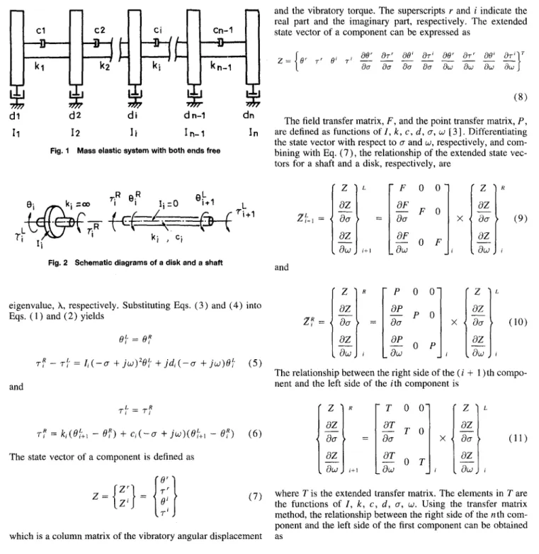
A mass elastic system with both ends free is shown in Fig. 1. The symbols / , k, c and d are the mass moment of inertia of a disk, the stiffness of a shaft, the internal damping coefficient and the external damping coefficient, respectively.
It is assumed that disks are rigid bodies with infinite stiff-nesses, that shafts are slender with negligible mass moments of inertia, that the damping effect is proportional to the relative vibratory angular speed, and that the damping coefficient is constant. The equations of motion for a disk and a shaft as shown in Fig. 2, respectively, are
0f- = 0f
r f - r f = /, ^ 0 , . + rf<^ (1)
rfr dt
and Tf = rf+iTf = A:,(0f;, - 0f) + c, 4 {®t^ - ©f) (2)
dtThe angular displacements and torques of stations can be ex-pressed as [6]
f 6\ + je\
9'2+jd'2 I 0:, + iO'n \ " J 't J { 0 ( 0 } = { > e = {Q{t)]e ( - f f + , ; u ) ( (3) and Tl + JT'z , r:, + JT'„ _> e i~o-^juj)l {T{t)}e (~a + jij)l (4)
{T(t)] = .
cl
D
-k i C2 k2 C l ki -jm W7 'W' d i d2 d i cn-1 kn-1 dn-1 ^ dn I I I2 l i I n - 1 InFig. 1 Mass elastic system witli botli ends free
and the vibratory torque. The superscripts r and ; indicate the real part and the imaginary part, respectively. The extended state vector of a component can be expressed as
9' r' 36' dr' dB' dr' d9' dr' 09' dr' da da da da dui du> du du
(8)
The field transfer matrix, F, and the point transfer matrix, P, are defined as functions of/, k, c, d, a, u> [ 3 ] . Differentiating the state vector with respect to a and ui, respectively, and com-bining with Eq. ( 7 ) , the relationship of the extended state vec-tors for a shaft and a disk, respectively, are
T^ e;R
eh
ki , Ci
Fig. 2 Schiematic diagrams of a disl< and a sliaft
Zi
r z 1
dZ < da dZ . i ^ t ^ , L, ~
1+1 OF da OF 0 0"^ F 0 0 F X . 1r z 1
dZ da \ dZ (9) andeigenvalue, \, respectively. Substituting Eqs. (3) and (4) into Eqs. (1) and (2) yields
0f = ef
Tf-T'^ = Id-<T+jt^ydi+jdi(-a +JLj)e'- (5) andZf
' z • dZ < da dZ . dijj, R > =/
P 0 dp da ^ 0 duj 0 " 0 P X . ' z • dZ da dZ (10)The relationship between the right side of the {i + 1 )th compo-nent and the left side of the (th compocompo-nent is
T'^^T^
T^ = kiei, - ef) + c:(~a+jujKeu^ - ef) (6)
The state vector of a component is defined asZ-<^:}=< T (7)
r z ]
dZ < da dZ duj J R>
i + i TOO' 3 ^ T- n d^ ' 'f 0 ^
duj X .' ^ 1
dZ da dZwhich is a column matrix of the vibratory angular displacement as
(11)
where T is the extended transfer matrix. The elements in T are the functions of /, k, c, d, a, to. Using the transfer matrix method, the relationship between the right side of the wth com-ponent and the left side of the first comcom-ponent can be obtained
N o m e n c l a t u r e A = matrix product a, b, e, g, h = element in the matrix
c = internal damping coeffi-cient
d = external damping
coef-ficient
/ = mass moment of inertia
k = stiffness
T = torque matrix; transposed
transfer matrix or torque / = time
Z = state vector
Z = extended state vector
a = absolute value of real part of eigen- ij = ith row and y'th column element of
value
X. = eigenvalue of matrix 0 = angular displacement vector
0 = angular displacement magnitude
T = torque magnitude
a = phase angle
6 = external forced circular frequency ui = imaginary part of eigenvalue Subscripts e = external i = ith component matrix Superscripts c = cosine component i = imaginary part
L = left side of component
R = right side of component r = real part
da dr'' da
del
da dr' daar
du dr' dujdei
diodr_
du a-i\ 041 «51 « ? ! flsi 0121 «12 «22 «32 «42 fl52 fl62 ^72 082 092 Ol02 a i 3 «23 «33 «43 ^ 5 3 063 073 083 O93 O1O3 fl]12 O1I3 O122 O123 fll4 024 034 O44 0S4 064 074 084 O94 O104 0 [ | 4 Ol24 0 0 0 0 O i l 021 031 041 0 0 0 0 0 0 0 0 012 0 0 0 0 Ol3 022 023 032 042 0 0 0 0 033 043 0 0 0 0 0 0 0 0 Ol4 024 034 044 0 0 0 0 0 0 0 0 0 0 0 0 On 02I 031 041 0 0 0 0 0 0 0 0 012 0 0 0 0 0 0 0 0 Ol3 022 023 032 033 042 043 0 0 0 0 0 0 0 0 Ol4 024 034 044, dO'' da dr' daml
da dr' da dW_ dr' dujdei
dri
duj (12) Z j = AZ, (13)The elements of the matrix are functions of / , k, c, d, a and w. If the extended state vector at the left side of the first compo-nent is
Z t = {1 0 0 0 0 0 0 0 0 0 0 0 } ' ' and Eq. (14) is substituted into Eq. (12), we can get
(14)
1"
da du)dT'„ dT'„ .da dui
and substituting Eq. (15) into Eq. (17) yields
O6I Oioi Ogl O121 -fl21 - 0 4 1 (17) (18) T „ = 041 da dr', da dui dK du> da 9fl41 ^ da dan du! da2\ dw = 061 = Ogl — Oioi (15) If the right side of the «th component is free, the vibratory torque of the «th component is zero. Therefore, it can be written
and
T',Xcr, W) = 0
r'„(o-, w) = 0 (16)
Equation (16) is known as the eigenvalue equation of a damped system.
Using the Newton-Raphson method with
By using the trial and error method with assumed initial values of a, w, the accurate eigenvalues can be obtained when T'^, and r i in Eq, (17) converge.
If the system shown in Fig. 1 is the equivalent mass elastic system of a multi-cylinder engine, 6 stands for the excitation frequency and a, stands for the phase angle of the cylinder with respect to the first firing cylinder of an engine, the external torque can be expressed as
T . = T .^'•<*'-"/'
= (Te, cos «; COS 6t - Tel sln a, sin St)
+ jiTei COS a, sin 6t - T^i sin a, cos 6t) (19) The real part of the torque is
^[(T'ci + JT'ei)e''"] = Tel COS «/ COS 6t - T^ sin a, sin 6t
= Tei COS 6t + r% sin 6t
Hence, we have
T% = Tel c o s a,- = T'ei
and
Table 1 Mass moments of inertia of disi<s and stiffnesses of shafts for the first undamped system
tfw^^vwwv^ri^^fwvwww^'vwwwwvwwimn^vwm^^n
Station no. I (N-m-sQ k (MN-m/rad) 1 2 3 4 5 6 7 8 9 71.882 41.387 41.387 41.387 41.387 71.822 4401.1 1763.2 162.28 1.3614 1.3614 1.3614 1.3614 1.3614 2.1523 1.4789 0.8417 - Tei Sin Ui = (21)
similarly, the real part of the angular displacement is
R[(0'e, + 7^;:,)e'*'] = O'ei COS 6t - 0', sin 8t (22)
If a system is subjected to an external torque, the relationship between the right side of the nth component and the left side of the first component can be expressed as
T L 1 J > = fli ^1 e, g, / , «2 ^2 62 g2 fl tti h, e , g j fj ^4 ^4 e4 g4 / 4 , 0 0 0 0 1 (23)
where the elements in the matrix are functions of / , k, c, d, 6 and T(,. If both ends of a system are free, rli and T'„ are all equal to zero. Hence, we have
and fl20'l + 626*'i + /i2 = 0 04^'1 + e^O'i + hi = Q a,^'i + eid\ + h, = Q', (24) (25) The vibratory angular displacement of the first component can be determined from Eq. (24). Therefore, the vibratory angular displacements of all components can be determined.
Q^ 1.2 ^ 0.8 ? 0.4 > -0.4 •B -0.8 2:-1.2
first mode «currQnt
AHolzer X current •second mode ^ j^ n H d z e r 4 5 6 7 S t a t i o n niimber
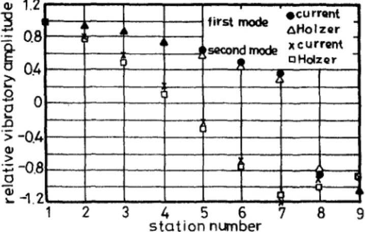
Fig. 3 Relative vibratory angular displacements of Vt\6 first undamped system
Table 2 Mass moments of Inertia and stiffnesses of ttie second un-damped system
VVVWVWVVSlv^VVVMyvVIIVWVyV|WWVVVWVVI<VV«VVVVWV»VVWVVV>n«VVVVWf¥VV»VI^^
station no.
I (N-m-sQ
k (MN-m/rad)
1 2 3 4 5 0.680 0.680 1.360 2.260 0.136 0.170 0.290 0.079 0.090 ^.^ !!!', « . „ «
-Table 3 Natural frequencies and relatively vibratory angular displace-ments of the second undamped system
1st mode 2nd mode .?.fd.5}.o.'?.6 ^t*!.!?}.'?.'?.^ current MATUB current MATLAB current MATLAB current MATLAB ffl atio no. 1 2 3 4 235 rad/s ti 1 0.78 0.55 -0.81 235 512 512 839 839 956 rad/s rad/s rad/s rad/s rad/s rad/s
relative vibratory angular displacement 1 1 I 1 1 1 0.78 -0.05 -0.06 -1.82 -1.82 -2.65 0.57 -0.63 -0.63 -0.47 -0.47 0.89 -0.83 0.09 0.06 10.16 10.21 -0.04 956 rad/s 1 -2.65 0.88 -0.04 -0.89 -0.91 0.15 0.13 -160.1 -161 0.11 0.11 Results
The first system with the mass moments of inertia of disks and the stiffnesses of shafts of a six-cylinder engine with a flywheel and a converter listed in Table 1 is used for analysis. It is assumed that the system is undamped with both ends free. There is a rigid mode with an eigenvalue equal to zero for a system with both ends free. The calculated natural circular frequencies of the top four modes are 1001, 1312, 2353 and 3677 rad/s. The first mode and the second mode obtained by using the Holzer method are 1030 and 1330 rad/s, respectively. The top four natural circular frequencies obtained by using the MATLAB software program are 1003, 1336, 2354 and 3811 rad/s, respectively. The results of the relative vibratory angular displacements for the first and the second mode shapes are shown in Fig. 3.
The mass moments of inertia of disks and the stiffnesses of shafts of the second undamped system with both ends free are shown in Table 2. The results of eigensolutions of the second undamped system obtained from this analysis and from the MATLAB software program are shown in Table 3.
The mass moments of inertia, the stiffnesses and the damping coefficients of the third damped system obtained from Doughty
Table 4 Mass moments of inertia and stiffnesses of the third undamped system •W(WVWWVWWV«V*VI«VW I k e d station no.
i
2 3 0.4 — — 6 0.3 0.5 8000 10000 10 0 0 0and Vafaee [6] with both ends free are shown in Table 4. The calculated results of the eigensolutions and the data obtained from Doughty and Vafaee [6] are shown in Table 5.
The fourth damped system with the mass moments of inertia, the stiffnesses and the damping coefficients of an engine with a generator obtained from Doughty and Vafaee [6] are shown in Table 6. Both ends of the damped system are free. The results of the eigensolutions for the system are shown in Table 7.
The mass moments of inertia and the external damping coef-ficients of disks, and the stiffnesses and the internal damping
Table S Results of the eigensolutions for the third damped system Table 8 Mass moments of inertia, stiffnesses and damping coefficients of the forced system
current calculated
results
Doughty and Vafaee's
results
stat-ion
no.
I
2
3
first mode second mode first mode
A*~ A ~ A."
-12.1+J161.3 -19.6+J246.3 -12,l+jl61.3
rad/s rad/s rad/s
second mode
X.=
-19.6+J246.3
rad/s
relative vibratory angular displacement
real imag real imag real imag
1.0 1.00 1.0
0.03 0.05 -1.21 0.33 0.03 0.05
-0.77 -0.14 0.79 -0.36 -0,77 -0.14
real imag
1.00
-1.21 0.33
0.79 -0.36
Table 6 Mass moments of inertia and stiffnesses of the fourth damped system tfW^tfWV^WWVWVWWWArtrfWVW^Wl^Art'VW^A^^^^AA'VVMnnAfWW^MWArVt^WmKWM^rtMAA^'
Station
no.
I (N-m-s^)k
(MN-m/rad) C (N-m-s/rad)d
(N-m-s/rad)1
2
3
4
5
6
7
8
9
10
11
12
6
4.5
4.5
6
6
4.5
4.5
6
3.5
100
20
350
16
16
16
13
16
16
16
25
150
0.5
10
-330550
Table 7 Results of the eigensolutions for the fourth damped system
Doughty
and
Vafaee's
results
current calculated
results
station
no.
1st mode 2nd mode 3rd mode 3rd mode
A; — A. A, A*
•1.6+j67,4 -0.3+J376.7 -8.0+j743,2 -8.0+J743.2
(rad/s) (rad/s) (rad/s) (rad/s)
1
2
3
4
5
6
7
8
9
10
11
12
real
1.00
1.00
1.00
0.99
0.98
0.98
0.97
0.96
0.95
0.95
-0.32
-0.38
relative vibratory angular displacement
imag real imag real imag real
0.00
-0.00
-0.00
-0.00
-0.00
-0.00
-0.00
-0.00
-0.00
-0.00
-0.01
-0.01
1.00
0.95
0.86
0.73
0.53
0.34
1.31
-0.08
-0.21
-0.23
-0.01
0.02
0.00 -0.00 -0.00 -0.00 -0.00 -0.00 -0.00 -0.00 -0.00 -0.00 -0.00 0.001.00
0.79
0.46
0.06
-0.45
0.00
-0.00
-0.01
-0.02
-0.02
-0.77 -0.02
-0.97 -0.01
-1.02
-0.92
-0.89
86.2
-4.65
0.00
0.02
0.02
-42.1
2.39
1.00
0.79
0.46
0.06
-0.45
-0.77
-0.97
-1.02
-0.92
-0.89
86.2
-4.65
imag
0.00
-0.00
-0.01
-0.02
-0.02
-0.02
-0.01
0.00
0.02
0.02
-42.1
2.39
station
no.
I
(N-m-s^)k
(MN-m/rad) C (N-m-s/rad)d
(N-m-s/rad)1
2
3
4
5
1.7
2.5
2.3
1.4
3.7
0.30
0.30
0.35
0.22
0.40
5600
8200
12000
4000
-0.0
0.0
0.0
9.9
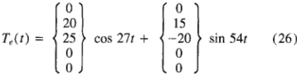
-coefficients of shafts in a system subjected to external torques
are shown in Table 8. If the disks of the system are subjected
to the external excitation torques,
TAt) = {
0
20
25
0
0
> cos 27/ + <
0
15
-20
0
0
sin 54/ (26)
it is known from Eq. (21) that the original coefficients of cos
27/ and the sign change of the original coefficients of sin 54/
in Eq. (26) should be used in the matrix. The angular
displace-ment of a components is
0(t) = U, cos 27/ + Vt sin 27/
+ U2 cos 54/ + V2 sin 54/ (27)
The results of the vibratory angular displacements of the
com-ponents and the data obtained by Doughty [14] are shown in
Table 9.
Discussion
The derivatives of the vibratory angular displacements and
the vibratory torques are used directly in the Newton-Raphson
technique to calculate the eigenvalues. The results are based on
the first order of approximation in the Newton-Raphson method.
If rJi and T'„ in Eq. (17) are less then lO"*" N.m, the values are
assumed to be converged.
This method eliminates the operation of the inverse matrix
because the derivatives of angular displacement and the torque
are used directly with the Newton-Raphson technique to
calcu-late the eigenvalues of systems. In addition to the zero elements,
there are 80 elements in the transfer matrix in Eq. (12).
Never-theless, only six elements, ajii <5!4i, flei. as\, flioi and ant, are
needed for Eq. (18) to calculate the eigenvalues. It is not
neces-sary to calculate all elements of the transfer matrix. Therefore,
using the Newton-Raphson technique with complex numbers in
the extended transfer matrix method should be better than using
the conventional transfer matrix method and then applying the
Table 9 Results of the coefficients of trigonometric functions
Angular Displacement (10 ) rad
station
no.
1
2
3
4
5
current calculated
results
Doughty's
results
U,
2.47
1.93
-1.31
-5.42
-16.3
U2-1.48
-0.16
0.89
1.10
-0.18
V,
1.33
1.03
0.60
0.22
-1.69
V24.33
0.50
-4.39
-3,61
2.23
U,
2.47
1.93
-1.31
-5.42
-16.3
U2
-1.48
-0,16
0.89
1.10
-0,18
V,
1.33
1.03
0.60
0.22
-1.69
V24.33
0.50
-4.39
-3.61
2.23
Newton's equation to determine the eigenvalues of a system. However, there is no computer running time available from the conventional transfer matrix method. In the meantime no computer time can be recorded in the personal computer for comparison.
There are some disadvantages of using this methodology. An initial eigenvalue is required to calculate one eigenvalue of a system. Improperly assumed initial values of a and w may result in the overshooting that leads to difficulty in determining some eigenvalues. For an undamped system, the residual torque con-verges quickly. Since the deviation of eigenvalues for the damped system from the system with the damping coefficients assumed to be zero is small for the most cases, the eigenvalues obtained for the system with the damping coefficients assumed to be zero are the best assumed initial values for damped sys-tems. Only one eigenvalue can be obtained at one time. If there are three eigenvalues for a system, it is necessary to assume three different initial eigenvalues. However, if only the natural frequency near the operation frequency is concerned for a steady running system, such as a turbine generator system, this method-ology is sufficient and adequate to analyze the torsional vibra-tion of the system.
For the first and the second undamped systems, the imaginary parts of the eigenvalues are zero, and no phase angle exists. The calculated results of the first and the second systems agree very well with the results obtained by using both the Holzer method and the MATLAB software program. The calculated results of the third and fourth damped systems show very good agreement with those obtained by Doughty and Vafaee [6] and Doughty [14]. Therefore, the methodology can be used for not only undamped systems but also damped systems subjected to external torques. It can also be used to analyze the torsional vibration for both steady systems and dynamics systems. The application range of the extended transfer matrix method with the Newton-Raphson technique is improved.
Acknowledgments
The authors would thank the National Science Council of the Republic of China for the Grant NSC80-0401-E002-21 to
complete this research project and to Grant D. Huang for com-ments and revisions made on this manuscript.
References
[ 1 ] Holzer, H„ Die Berechnung der Drehschjwingungen, Springer, Berlin, 1922.
[2] Den Hartog, J. P., and Li, J. P., "Farced Torsional Vibrations with Damping; An Extension of Holzer's Method," ASME Journal of Applied Me-chanics, Dec. 1964, pp. 276-280.
[3] Pestel, B.C. and Leckie, F. A., Matrix Methods in Elasto Mechanics, McGraw-Hill, New York, 1963.
[4] Eshleman, R. L., "Torsional Response of Internal Combustion Engines," k^yK, Journal of Engineering for Industry, Vol. 96, May 1974, pp. 4 4 1 -449.
[51 Sankar, S., "On The Torsional Vibration of Branches System Using Extended Transfer Matrix Method," ASME Journal of Engineering for Industry, Series B, Vol. 101, Oct. 1979, pp. 546-553.
[6] Daughty, S., and Vafaee, G., "Transfer Matrix Eigensolutions for Damped Torsional System,'' ASME JOURNAL OF VIBRATION, ACOUSTICS, STRESS,
AND RELIABILITY IN DESIGN, Vol. 107, Jan. 1985, pp. 128-132.
[7] Dawson, B., and Davies, M., "An Improved Transfer Matrix Proce-dure," International Journal for Numerical Methods in Engineering, Vol. 8, 1974, pp. 111-117.
[8] Doughty, S., " A Rayleigh-Type Inclusion of Shaft Inertia in Torsional Vibration Analysis," ASME Journal of Engineering for Gas Turbines and Power, Vol. 116, Oct. 1994, pp. 831-837.
[9] Neilson, R. D., and Barr, A. D. S., "Imbalance Effects in Rotor Systems under High Angular Accelerations," ASME Proceedings of International Gas Turbine and Aeroengine Congress and Exposition, paper 21091, 1994, pp. 1-10.
[ 10] Yun, Jong-Seop, and Lee, Chong-Won, "Dynamic Analysis of Flexible Rotors Subjected to Torque And Force," ASME Proceedings of the 14th Biennial ASME Design Technical Conference on Mechanical Vibration and Noise, DE v60, 1993, pp. 331-338.
[11] Lu, Songyuan,' 'Transfer Matrix Method for Nonlinear Vibration Analy-,sis of Rotor-bearing System," ASME 13th Biennial Conference on Mechanical Vibration and Noise, DE, Vol, 37, 1991, pp. 7 5 - 8 3 .
[ 12] Kang, Yuan, and Chung, Yung Being, "Transfer Matrix Method for the General Periodic Torsional Vibration of Rotor Systems,'' ASME Proceedings of the 2nd Biennial European Joint Conference on Engineering Systems Design and Analysis, Part 7 (of 8) PD, Vol. 64, No. 7, 1994, pp. 195-202.
[13] Huang, Y. M., "Performance of the Damper in a Power Train," ASME paper No. 84-DET-160, 1982.
[14] Doughty, S., "Steady-State Torsional Responnse with Viscous
Damp-ing," ASME JOURNAL OF VIBRATION, ACOUSTICS, STRESS, AND RELIABILITY IN