DESIGN OF INTEGRAL VARIABLE STRUCTURE CONTROLLER AND APPLICATION TO ELECTROHYDRAULIC VELOCITY SERVOSYSTEMS

(1)

Design

of

integral variable structure controller and

application to electrohydraulic velocity

servosystems

T.-L. Chern

Y.-c.

w u

Indexing terms; Control systems, Integral variable structure control, Servosystems

Abstract: An integral variable structure controller (IVSC) for robust servotracking is proposed. It comprises an integral controller, which is designed for achieving zero steady-state error under step input, and a variable structure controller (VSC) which is designed for enhancing robustness. A procedure is developed for determining the coefi- cients of the switching plane and the integral control gain such that the overall closed-loop system has the desired eigenvalues. Furthermore, a modifed proper continuous function is introduced to overcome the chattering problem. An electrohydraulic velocity servocontrol system using the proposed IVSC approach is illustrated. Simulation results show that the proposed IVSC approach can achieve accurate servotracking and is fairly robust to plant parameter variations and external load disturbances.

1 Introduction

The most distinct feature of the variable structure con- troller (VSC) is the existence of a sliding mode which occurs on a predetermined switching plane [l-31. Once in sliding mode, the system will be forced to slide along, or at the vicinity of, the switching plane and hence is theoretically robust to plant parameter variations. However, a controller based on variable structure configuration may fail to meet the desired performance when the system is commanded to track an arbitrary or a step input, or is subjected to external disturbances. To solve this problem, we propose an IVSC approach which com- prises an integral controller followed by a variable structure controller. The design of such a system involves the determination of the switching plane, the integral control gain and the control function to guarantee the existence of a sliding mode.

The performances of the proposed IVSC approach, the conventional VSC and the linear approach have been compared by computer simulation, with an electrohydraulic velocity control system as an illustration. The dynamics of this type of system are usually very complex and highly nonlinear due to the flow-pressure relation- Paper 8074D (C9), first received 18th April and in revised form 21st November 1990

T.-L. Chern is with the Institute of Electronics, National Chiao Tung University, Hsinchu, Taiwan, Republic of China

Y.-C. Wu is with the Institute of Control Engineering, National Chiao Tung University, Hsinchu, Taiwan, Republic of China

IEE PROCEEDINGS-D, Vol. 138, N o . 5 , SEPTEMBER 1991

ship [4, 51. The simulated results show that the proposed IVSC approach can almost maintain an identical response in the face of large plant parameter variations and external disturbances. It yields improved per- formance when compared to the conventional VSC and the linear approaches.

2

The proposed configuration of the IVSC combines an integral controller followed by a VSC, as shown in Fig. 1, and is described as follows:

Integral variable structure system (IVSS)

X i = i = 1, ..., n - 1

(14

n

x n =

- 1

aiXj

+

bU -f(t) i = l Z = r - X l integral controller vsc r 1 I

Fig. 1 Block diagram of an IVSS

where X , is the output signal, r is the input command, K is the gain of the integral controller, ai and b are the plant parameters, f ( t ) are disturbances, and the control function U is piecewise linear of the form

U + ( x , t ) if 0

>

0 U - ( X , t) if o < 0

where U is the switching function given by

n

U = c , ( X , - K Z )

+ l c i X i

ci = constant

i = 2

cn = 1 (3)

The design of such a system involves

(a) the choice of the control function U so that it gives rise to the existence of a sliding mode, and

(b) the determination of the switching function U and

the integral control gain K such that the system has the desired eigenvalues.

(2)

2.1 Choice of control function

From eqns. 1 and 3, we have

n ir = - c l K ( r - X , )

+

_{c i _ , X i} i = 2 -

2

a i X i

+

bU - f ( t ) i - 1 Let (4) a, = U?

+

Aai i = 1 , ..., n b = bo + Ab

where U: and bo are nominal values of a, and b, and Aai and Ab are the variations of a, and b, respectively.

Let the control function U be decomposed as

U = U,,

+

AU

( 5 4

where U,, , called equivalent control, is defined as the sol- ution of the problem ir = 0 under f(t) = 0, a, = a? and b = bo. That is

c , K ( r - X , ) - c i - , X i

+

f

@ X i ] / b o (5b)

i = 2 i = 1

AU is used to eliminate the influence due to the plant parameter variations in Aai, Ab and the disturbances f ( t ) to guarantee the existence of a sliding mode. This function is constructed as follows:

n AU = Y l ( X 1 - K Z )

+ 1

Y i X i i = 2 where if X i a > 0 if X,a < 0 Y i =

{;

i = 2,

...,

n

It is known that the condition for the existence of a sliding motion is [l]

lim air < 0

0-0

Substitution of eqn. 5 into eqn. 4 yields

n

.

- l A a i X i - f ( t ) + A b U , , + b A U i = 1 n = -

1

A a i X i - f ( t ) i = l n n

1 +

Ab/bo c l K ( r - X , ) -

1

ci- l X i

+

1

aPXi

i = 2 i = 1 n

1 [

Y l ( X 1 - K Z )

+

C Y i X i i = 2 Then ay Ab b - Aul

+

7

+

b Y l a0 Ab

+

[(

- A a i + + i = 2 b 0-0

+

b Y , X i a

> I

c i p l Ab bo -~ (7)

If we neglect the term N ( t ) { - K Z ( A a , - ay Ab/bo)

+

A b / b o [ c l K ( r - X I ) ] -f(t)},o in eqn. 8, then the conditions for satisfying the inequality (eqn. 6) are

a.

<

(Aa, - a? Ab/bo

+

ci-

,

Ab/bo)/b

> (Aai - a: Ab/bo

+

c i - , Ab/bO)/b

Yi =

{b:

i = 1,

...,

n co = O (9) However, the term N(t) may not be neglected in the pre- sence of an input command, the plant parameter variations and/or the external disturbances. Hence, once the effect of the term N ( t ) exceeds the other two terms in eqn. 8 so that the inequality of eqn. 6 is violated, then the sliding mode breaks down and the system gives rise to a limit cycle. Fortunately, by increasing the control gain Y i the effect due to the term N ( t ) can be arbitrarily sup- pressed so that the magnitude of the limit cycle can be reduced to within a tolerable range, the validity of the assumption can be shown by the simulation, and hence a quasi-ideal sliding motion can be obtained.

2.2 Determination of switching plane and integral

control gain

While in the sliding motion, the system described by eqn. 1 can be reduced to the following linear equations [l-31

X i = X i + l i = 1, ..., n - 2 ( 1 0 4

n - 1

X n - l = -

1

c i X i

+

clKZ

i = 1 i = r - X , or, in matrix form

X = A X + B r ( 1 1 ) where

c_

2-

1

X

x = l

. l

I

I-!

I

The closed-loop transfer function of the system described by eqn. 1 1 is

where R(S) and X , ( S ) are the Laplace transforms of r and

X , , respectively. The characteristic equation of the

IEE PROCEEDINGS-D, Vol. 138, NO. 5 , SEPTEMBER 1991

(3)

system is

S"

+

c , _ , S ~ - '

+

. . .

+

c 2 S Z

+

c , S

+

c , K = 0 (13)

Because this characteristic equation is independent of the plant parameters, the IVSC approach is robust to the plant parameter variations. It can achieve a zero steady- state error and its eigenvalues can be set arbitrarily. Let the desired eigenvalues of the system be I , , . .

.

,

I , , or an equivalent desired characteristic equation

S"

+

a l S n - l

+

+ a , = O

Then the switching plane coefficients ci for i = 1, .

.

.,

n - 1 and the integral control gain K can be chosen as

follows cnpl = a ,

c , =

3 Chattering

For the control law as given by eqn. 5, if Y i (i = 1,

. .

., n) are chosen as

y. = a . = -/j.

1 1

then the control function U can be represented as

n n

]Ib0

U = c , K ( r - X , )

+

z c i - , X i - C a y x i

+

(Y1 JXl - KZI

+

t Y i I X i l ) sign (a) (14)

Because the control U gives rise to chattering due to the sign function sign (a), direct application of such a control signal to the plant may be impractical. To obtain a continuous control signal, the discontinuous sign function sign (a) in eqn. 14 can be replaced by a proper continuous function

[b8]

as

c

i = 2 i = 1

i = 2

where 6 is a positive constant. However, under different operating conditions, the proper continuous function with a constant 6 may not effectively eliminate the chattering phenomena. For improving the result, 6 is chosen alternatively as a function of

1

X , - r

I

as

6 = 6,

+

6,1X1 - r I

where 6, and 6, are positive constants. Then the modified proper continuous function is given by

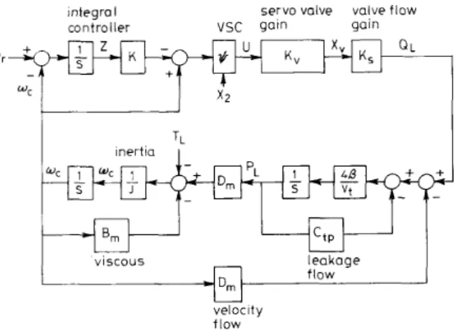
4 Electrohydraulic velocity control problem

The block diagram of the electrohydraulic velocity control system to be studied is shown in Fig. 2. The objective of the control is to keep the velocity w, of the hydraulic system following the desired trajectory as closely as possible, regardless of the operating points.

The relation between the valve displacement X , and the load flow rate Q L is governed by the well known orifice law given by [ 4 ]

QL = X, K j J [ P , - sign ( X , ) P L ] = X, K , (17) IEE PROCEEDINGS-D, Vol. 138, N O . 5 , SEPTEMBER 1991

where K j is a constant for a specific hydraulic motor, P , is the supply pressure, P L is the load pressure and K , is the valve flow gain which varies at different operating

integral servo valve valve flow

con t ro I ler vsc gain gain Q L K "

T l inertia i

PAW?l

viscous leakage

velocity flow

Fig. 2 Block diagram of a hydraulic velocity control system with

I

vsc

points. The flow continuity property of the servo valve and motor chamber yields

where D , is the volumetric displacement, C,, is the total leakage coefficient, is the total volume of the oil,

8

is the bulk modulus of the oil and w, is the velocity of the motor shaft. The torque balance equation for the motor is given by

where B , is the viscous damping coefficient and T L is the external load disturbance which is assumed to be dependent upon the velocity of the shaft or slowly time varying as described by

The above form of the external load disturbance can fre- quently be found in industrial processes [ S I involving hydraulic servo systems.

By combining eqns. 17-19, the servo valve gain K , and the IVSC, we obtain a set of state equations of the integral-variable-structure-controlled electrohydraulic servo system as follows :

where

X , = CO, is the velocity of the motor shaft K = the gain of the integral controller.

r = CO, is the reference input

(4)

I

Table 1 : System Darameters for simulation

Parameter Value Dimension

K s 2.3 x x J [ f , - sign (X,)P,] m2/s 1.4 x l o 7 Nt/m2 3.5 x i o 7 Nt/mz 3.3 x 10-5 m3/rad v , c*, 2.3 x l o - " m5/s/Nt D m 1.6 x 10-5 m3/rad J 5.8 x 10-3 kg-m-s2 B* 0.864 kg - m - s/rad K" 0.5 _m/v

B'.

Following the design procedure as described in the pre- vious Section, we obtain

U = [ c , K ( r - X , )

+

a y X ,

+

a; X21/bo

+

('4'1

I

x ,

- K Z

I

+

y 2

I

x ,

I

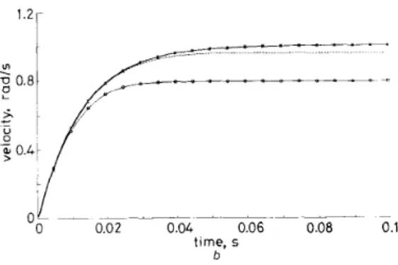
) M A O ) ( 2 2 4 1.2, . 0.02 0.04 0.06 0.08 0.1 time, s 0 1.21 , x

-

--

0.02 0.04 0.06 0.08 0 1 time, s b Ob-/ Fig. 3

For Ma(u), d = 20

+

1001X, - o,I

-0- IVSC -0- vsc

- x - linear

U TL = 0 kg-m

b TL = 20 I mc I kg-m

Velocity responses of IVSC, V S C and linear approaches

where ay, a; and bo are nominal values of a,, a, and b ; Aa,, Aa, and Ab are the deviation from ay, a: and bo,

respectively, and

Yi

< -

I

Aai

-

a: Ab/bo

+

ci -

,

Ab/bO

I

/b

i = 1 , 2 co = 0 (22b) The c function is obtained from eqn. 3 as

U = c l ( X l - K Z )

+

X , ₍₂₃₎

In the sliding motion, the system described by eqn. 21 can be reduced to the following simple linear form

X , = - c l ( X , - K Z )

i = r - X ,

The characteristic equation of this reduced system is

S2

+

c , S

+

c,K = 0 (25)

It is clear that the dynamic performance of the system can now be determined by simply choosing the coefficient c, and the gain K . Let the characteristic equation of the system with desired eigenvalues 1, and

1,

be

sz

-

(A,

+

A,)S

+

Alaz

= 0

Then c1 and K can be chosen as

5 Simulation results and discussion

The robustness of the proposed IVSC approach against large variations of plant parameters and external load disturbances have been simulated for demonstration. The results were compared to those obtained by a conven- tional VSC and

a

conventional linear controller. The nominal values of the hydraulic system parameters are listed in Table 1 . By considering different operating points, we assume the range of the plant parameter variations to be

1

Au,

1

< U? x 500%

(Ab1 < b o x 500%

Choosing the poles of the system as described by eqn. 24 at - 100 f j80, we obtain the coefficients of the switching

plane and the integral control gain given by eqn. 27 as c1 = 200 and K = 82.

Thus, from eqn. 22b, the gains

Y ,

and Y, must be

chosen to satisfy the following inequalities :

'4'1 < - 0.48 '4'2

<

- 0.00057

Based on simulations, one possible set of switching gains is chosen as follows:

'4'1 = -0.7 Y Z = -0.002

This IVSC design gives a control function U = [ c , K ( r - X I )

+

a y X l

+

a ; X 2 ] / b o

where Md(o) is given by eqn. 16 and o = 2OO(X, - K Z )

+

x,.

A conventional VSC approach is presented for per- formance comparison. In this approach, let the control function U be

U = [8O(X, - r)(80 - a;)

+

X l a ? l / b o

+

(-0.5

I

X , - r

I

- 0.001

I

X , I)Ma(a)

where U = 8 q X , - r)

+

X , . Also a conventional linear controller with the transfer function

2.06 S

+

200 S

+

48.3

(s

S + 56.8

has been chosen for comparison. It was designed with the aims of matching and dynamic response of the IVSC

approach by means of a computer-aided technique

[SI.

The simulation results of the dynamic responses under various operating conditions are plotted in Figs. 3-7. Fig. 3 shows the dynamic responses of the three approaches when a shaft-velocity-dependent external load dis-

(5)

turbance TL is present. It is clear that the response can almost be maintained for the IVSC approach, whereas it varies significantly for both the linear and the VSC approaches. Fig. 4 shows the dynamic responses of the three approaches under a constant external load dis-

0 0.02 0.04 0.06 0.08 0.1

time, s

Fig. 4

TL = 20 kg-m, input command o, = 0 rad/s and function Ma(u), 6 = 20 + 100 1 X , - w.1

-0- IVSC --0- vsc

- x - linear

Velocity responses ofthe I V S C , V S C and linear approaches

0.6 r 0 0.02 0.06

I

t

0.02

5 oI?/

" 3 ' - 0 . 0 2 , -0.06 - 0 0.02 , , , , 0.04 0.06 0.08 0.1 time, s a ~ - _ ~ _ _ _ _ , , , , 0.04 0.06 0.08 0.1 time, s b Fig. 5 a without Ma(@, d = 0

b with Ma(u), 6 = 20 + 1001X, - w,I

Control signal in the IVSC approach with w, = 1 radlsec

turbance. Results show that the IVSC approach results in fast convergence to the zero steady-state, but the other two approaches give rise to significant deviations and/or steady-state errors. Thus, we conclude that the proposed IVSC approach is robust to the external load dis- turbances.

Fig. 5 shows the waveforms of the control function U . It is clear that by using a modified proper continuous function, chattering phenomena can be eliminated and the strength of the control signal can also be significantly reduced. Thus, the IVSC approach seems amenable for practical implementation. Fig. 6 shows the dynamic responses of the IVSC approach under different values of IEE PROCEEDINGS-D, Vol. 138, NO. 5 , SEPTEMBER 1991

6. It is obvious that the proposed approach with the value of 6 dependent on

I

X - I

I

is robust to the differ-

ent input command levels. 1.2

I

t

_ - . . . . , 0.1 0 ; 0 0.02 0.04 0.06 0.08 time, s 0 0.12r O ' A L p - -

--

- - , ' , 0 0.02 0.04 0.06 0.08 0 1 time, s b Fig. 6 of 6 -0- 6 = 0 -0- 6 = 1 0 0 - x - 6 = 2 0 + 1001X, --,I a o, = 1 rad/s b o, = 0 1 rad/s

Velocity responses ofthe IVSC approach under d%ferent values

Fig. 7 shows the dynamic responses of the three approaches under changes of the servo valve gain K , , inertia J and total leakage coefficient C t p , respectively. From the observations, we conclude that the IVSC approach is also insensitive to the variations of the parameters K , , J and C t p . This conclusion agrees with that predicted by the characteristic equation as given by eqn. 25 which should be independent of the plant parameters.

6 Conclusion

Most practical control systems are usually required to track an input signal in the presence of external dis- turbances. In this paper we have presented an IVSC con- figuration and developed a procedure for determining the coefficients of the switching plane and the integral control gain. It was shown in Section 2 that the IVSC approach is theoretically robust to the plant parameter variations. It can achieve a zero steady-state error for step input and its eigenvalues can be set arbitrarily. To solve the chattering problem, we also introduced a modified proper continuous function which can eliminate chattering under different operating conditions. An electrohydraulic velocity control problem was used to demonstrate the design procedure of the IVSC approach. Simulations showed that the proposed approach can give accurate servotracking response in the face of large plant parameter variations and external disturbances. It is a robust and practical control law for servomechanism systems.

(6)

I 1.2, 1.21 O M , . , , , , , ,

-_

0 0.02 0.04 0.06 0.08 0.1 time, s a

f i

I

/

\

- _ _ _ - 0.02 0 0 4 0.06 008 0 1 - - _ _ _

-

O d H . 0.02 ’ ’ 0.04 0.06 0.08 0.1 time, s C 7 References

1 UTKIN, V.I.: ‘Variable structure systems with sliding modes’, IEEE 2 UTKIN, V.I.: ‘Sliding modes and their application in variable struc- 3 ITKIS, U.: ‘Control systems of variable structure’ (John Wiley, 1976) 4 MERRIT, H.E.: ‘Hydraulic control system’ (John Wiley, 1967) 5 Yun, J.S., and CHO, H.S.: ‘Adaptive model following control of elec-

trohydraulic velocity control systems subjected to unknown dis- turbances’, IEE Proc. D, Control Theory & Appl., 1988, 135, pp.

Trans., 1977, AC-22, pp. 212-222 ture systems’ (Mir: Moscow, 1978)

149-156

time, s

b

Fig. 7 Velocity responses of the IVSC, V S C and linear approaches under changes of the servo valve gain K , , inertia J and leakage coejicient

r

IP

n IVSC approach with function Ma(“), 6 = 20 + 1001 A’, - w,l -0- normal

-0- -50% changes in K , - x -

~~~~ 100% changes in C,,

b VSC approach with function Mgo). 6 = 20

+

1001 X , ~ w,I -0- normal -0- -SO”/” changes in K , -- x - ~~-~ 100% changes in C, , c Linear approach -0- normal -0- - x - 500% changes in J 500% changes in J - 50% changes in K , 500% changes in J 100% changes in C , ,

6 AMBROSINO, G., GELENTANO, G., and GAROFALO, F.: ‘Vari- able structure model reference adaptive control system’, Int. J. Contr., 7 HASHIMOTO, H., MARUYAMA, K., and HARASHIMA, F.: ‘A

microprocessor-based robot manipulator control with sliding mode’,

IEEE Trans., 1987, IE-34, pp. 11-18

8 YUNG, K.D.: ‘A variable structure model following control design for robotics applications’, IEEE Trans., Robot. Autom., 1988, 4, pp. 556561

9 ASHWORTH, LT. CDR. M.J., and TOWILL, D.R.: ‘Computer- aided design of tracking systems’, Radio & Electron. Eng., 1978, 48, pp. 479492

1984,39, pp. 1339-1349