A holographic projection system with an
electrically tuning and continuously adjustable
optical zoom
Hung-Chun Lin,1 Neil Collings,2,* Ming-Syuan Chen,1 and Yi-Hsin Lin1 1Department of Photonics, National Chiao Tung University, 1001 Ta Hsueh Rd., Hsinchu 30010, Taiwan 2Electrical Engineering Division, University of Cambridge, 9 JJ Thomson Ave, Cambridge CB3 0FA, UK
Abstract: A holographic projection system with optical zoom is
demonstrated. By using a combination of a LC lens and an encoded Fresnel lens on the LCoS panel, we can control zoom in a holographic projector. The magnification can be electrically adjusted by tuning the focal length of the combination of the two lenses. The zoom ratio of the holographic projection system can reach 3.7:1 with continuous zoom function. The optical zoom function can decrease the complexity of the holographic projection system.
©2012 Optical Society of America
OCIS codes: (230.3720) Liquid-crystal devices; (230.2090) Electro-optical devices; (230.6120)
Spatial light modulators. References and links
1. A. Georgiou, J. Christmas, J. Moore, A. Jeziorska-Chapman, A. Davey, N. Collings, and W. A. Crossland, “Liquid crystal over silicon device characteristics for holographic projection of high-definition television images,” Appl. Opt. 47(26), 4793–4803 (2008).
2. E. Buckley, “Holographic laser projection,” J. Disp. Technol. 7(3), 135–140 (2011). 3. E. Buckley, “Holographic projector using one lens,” Opt. Lett. 35(20), 3399–3401 (2010).
4. M. Makowski, I. Ducin, K. Kakarenko, A. Kolodziejczyk, A. Siemion, A. Siemion, J. Suszek, M. Sypek, and D. Wojnowski, “Efficient image projection by Fourier electroholography,” Opt. Lett. 36(16), 3018–3020 (2011). 5. M. Makowski, M. Sypek, I. Ducin, A. Fajst, A. Siemion, J. Suszek, and A. Kolodziejczyk, “Experimental
evaluation of a full-color compact lensless holographic display,” Opt. Express 17(23), 20840–20846 (2009). 6. B. Marx, “Holographic optics - Miniature laser projector could open new markets,” Laser Focus World 42, 40
(2006).
7. T. Shimobaba, A. Gotchev, N. Masuda, and T. Ito, “Proposal of zoomable holographic projection without zoom lens,” in Proc. Int. Disp. Workshop, (Nagoya, Japan, 2011), PRJ3.
8. M. Kawamura, M. Ye, and S. Sato, “Optical particle manipulation using an LC device with eight-divided circularly hole-patterned electrodes,” Opt. Express 16(14), 10059–10065 (2008).
9. M. Nazarathy and J. Shamir, “Fourier optics described by operator algebra,” J. Opt. Soc. Am. 70(2), 150–159 (1980).
10. J. W. Goodman, Introduction to Fourier Optics, 2nd ed. (New York: McGraw-Hill, 1996).
11. A. Georgiou, J. Christmas, N. Collings, J. Moore, and W. A. Crossland, “Aspects of hologram calculation for video frames,” J. Opt. A, Pure Appl. Opt. 10(3), 035302 (2008).
12. M. Ye and S. Sato, “Optical properties of liquid crystal lens of any size,” Jpn. J. Appl. Phys. 41(Part 2, No. 5B), L571–L573 (2002).
13. Y. H. Lin, M. S. Chen, and H. C. Lin, “An electrically tunable optical zoom system using two composite liquid crystal lenses with a large zoom ratio,” Opt. Express 19(5), 4714–4721 (2011).
14. U. Schnars and W. P. O. Juptner, “Digital recording and numerical reconstruction of holograms,” Meas. Sci. Technol. 13(9), R85–R101 (2002).
15. A. F. Naumov, G. D. Love, M. Y. Loktev, and F. L. Vladimirov, “Control optimization of spherical modal liquid crystal lenses,” Opt. Express 4(9), 344–352 (1999).
16. B. Wang, M. Ye, M. Honma, T. Nose, and S. Sato, “Liquid crystal lens with spherical electrode,” Jpn. J. Appl. Phys. 41(Part 2, No. 11A), L1232–L1233 (2002).
17. M. Ye, B. Wang, and S. Sato, “Realization of liquid crystal lens of large aperture and low driving voltages using thin layer of weakly conductive material,” Opt. Express 16(6), 4302–4308 (2008).
19. H. C. Lin and Y. H. Lin, “An electrically tunable-focusing liquid crystal lens with a low voltage and simple electrodes,” Opt. Express 20(3), 2045–2052 (2012).
20. H. Ren and S. T. Wu, Introduction to Adaptive Lenses (John Wiley & Sons Ltd. 2012). 1. Introduction
A conventional projector is based on imaging an amplitude modulated microdisplay in the far field. The holographic projector generates an image on a screen using diffraction. It uses a spatial light modulator (SLM) to shape the wave front of the incident light and generate the image by diffraction [1–3]. One advantage of the holographic projector is its high light efficiency due to the use of a laser light source. Although the holographic projector has better color rendering due the narrow bandwidth of the laser source, it is more sensitive to the wavelength of the source compared to the conventional projector [4–6]. For a color holographic projector, image mismatch between the different colors may easily occur due to the wavelength dependence. In this paper, we will demonstrate the use of a liquid crystal (LC) lens to control zoom in a holographic projection system. This could be used to perform color correction by simply changing the focal length of the LC lens and an encoded Fresnel lens on the SLM. The zoom function not only reduces the hologram calculation load [7], but also provides a straightforward control of the image magnification. Image position can also be controlled with split electrode LC lens, although this is not demonstrated here [8].
2. Structure and operating principles
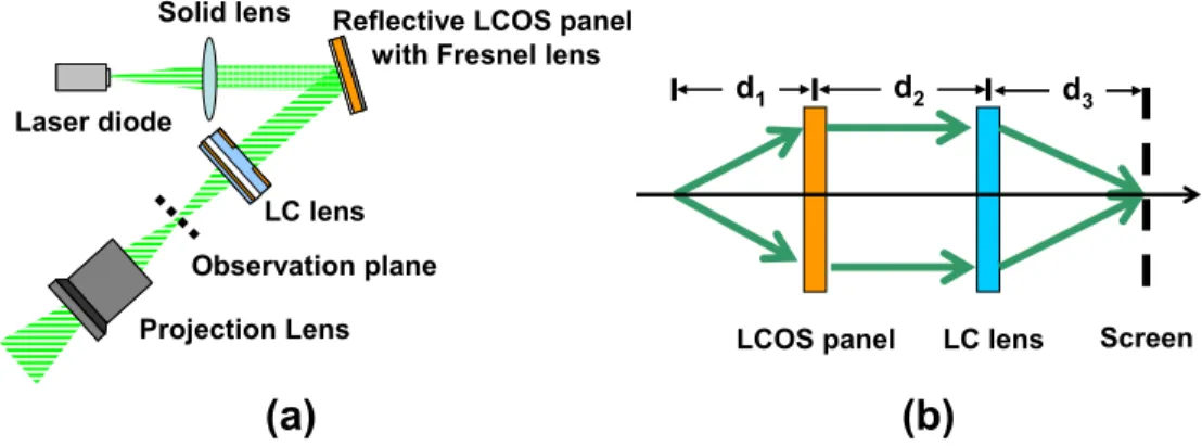
In order to realize a tuning holographic projection system, we add a LC lens to a Fourier holographic projector in which a Fresnel lens encodes lens power. Figure 1(a) shows the structure of the designed optical system consisting of a laser diode (λ = 532 nm), a solid lens, a reflective liquid crystal on silicon (LCoS) panel, a LC lens, and a projection lens. A green laser diode and a solid lens are used to generate a collimated coherent light source. The laser beam illuminates a reflective LCoS panel and then passes through the LC lens. The polarization of the laser beam is set parallel to the rubbing direction of the LCoS panel and the LC lens. The system includes two electrically tuning lenses: one is the Fresnel lens encoded on the LCoS panel and the other is the LC lens. The Fourier transform of the hologram displayed on the LCoS panel will be formed in the effective back focal plane (observation plane in Fig. 1(a)) of the optical system due to Fraunhofer diffraction. The projection lens reimages the pattern to the screen. The projection lens can increase the diffraction angle and magnify the Fraunhofer diffraction pattern. In order to simplify the discussion, we put a screen in the observation plane in order to observe the intermediate image formed by the two electrically tuning lenses.
The effective optical system of Fig. 1(a) is depicted in Fig. 1(b), where we have omitted the solid lens and the projection lens. The light source is the spherical wave originating at a distance d1 from the LCoS panel. When the light source is perfectly collimated, d1 equals
infinity. The distance between the LCoS panel and the LC lens is d2, and the distance between
the observation plane and the LC lens is d3. We will follow the Nazarathy and Shamir
operator method for analyzing the coherent optical system [9,10]. Since the LCoS panel is both displaying the Fourier hologram f(x,y) and encoding the Fresnel lens with the focal length fF, the operator for the LCoS panel f’ can be expressed as
1 ' ( , ) [ ], F f f x y Q f = − (1)
where Q is the operator for the multiplication by a quadratic-phase exponential. Therefore, the transform operator T of the optical system can be expressed as
3 2 1 1 1 [ ] [ ] [ ] ' [ ], LC T R d Q R d f Q f d = − (2)
where R is the operator for free-space propagation. By using the relations between the operators, we can simplify Eq. (2) to the following equation
2 3 3 3 2 3 3 3 3 1 2 2 3 3 1 1 [ ( ) ] 1 1 1 1 [ ] [ ]. ( ) LC LC LC LC LC LC LC LC LC F LC LC f T Q d f d f f d d f d f V Ff Q d f d f f d d d f d f d f d λ = + ⋅ ⋅ − − + − ⋅ ⋅ ⋅ ⋅ ⋅ ⋅ − + − + + − − (3)
In Eq. (3), operators F and V are the Fourier transform and scaling by a constant respectively. From Eq. (3), we can ignore the first Q operator since the phase function will not modulate the observed image. In order to obtain the Fraunhofer diffraction pattern, the second Q operator is then set to be unity, which means that
1 3 2 3 1 2 3 1 2 3 1 3 1 2 . ( ) F F LC F d d f d d f d d d f f d d d d d d d ⋅ ⋅ + ⋅ ⋅ − ⋅ ⋅ = + + − ⋅ − ⋅ (4)
Therefore, the transform operator T can be rewritten as
2 2 3 3 [ ] . ( ) LC LC LC f T V Ff d f d d d f λ = ⋅ ⋅ − ⋅ + ⋅ (5)
Let M = λ[d2 + d3-d2 × d3(1/fLC)]; then, the output image at the observation plane U(ξ,η) can
be expressed as [9,10] 1 ( , ) ( , ) exp[ 2 ( )] , U f x y j x y dxdy M M M ξ η ξ η =
− π + (6)where M is seen to be the magnification of the output image. The Fourier transform of the hologram f(x,y) will be formed at the distance d3 with the magnification M. Since all the
optical components of the system are fixed in position, which means that d1, d2 and d3 are
constant, the magnification of the intermediate image depends on the focal length of the LC lens fLC. To keep the Fourier plane at the same distance d3, the focal length of the Fresnel lens
encoded on the LCoS panel can be expressed as
1 2 3 1 2 1 3 1 3 2 3 1 2 3 . ( ) LC LC F LC d d d d d f d d f f d d d d f d d d ⋅ ⋅ − ⋅ ⋅ − ⋅ ⋅ = ⋅ + ⋅ − + + (7)
Since the focal lengths fLC and fF are electrically tunable, we can simply adjust the
magnification of the image by adding a LC lens to the conventional holographic projector. The structure is feasible and without computational complexity.
Laser diode
Solid lens Reflective LCOS panel with Fresnel lens
Projection Lens LC lens Observation plane
d1 d2 d3
LCOS panel LC lens Screen
(a)
(b)
Laser diode
Solid lens Reflective LCOS panel with Fresnel lens
Projection Lens LC lens Observation plane
d1 d2 d3
LCOS panel LC lens Screen
(a)
(b)
Fig. 1. (a) The structure of the holographic projection system using a liquid crystal lens. (b) The schematic of effective optical system of (a) d1 is the effective radius of curvature of the
incident light. 3. Experiment and results
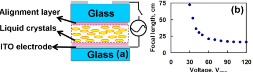
To demonstrate a holographic projector with controlled zoom, we adopt the reflective LCoS panel (LC-R 1080, HOLOEYE) and a LC lens with 2 mm aperture. The resolution of the LCoS panel is 1920 x 1200 with pixel pitch 8.1 μm. A line image of Bart Simpson was used (copyright held by activitycoloringpages.com) because deficiencies in the black background are readily apparent, and allow direct comparison between different reconstruction scenarios. The hologram was calculated by an iterative Gerchberg Saxton algorithm [11]. The structure of the LC lens was based on the hole-patterned electrode as shown in Fig. 2(a) [12]. The structure of the LC lens consists of two indium tin oxide (ITO) glass substrates of thickness 0.55 mm, and a LC layer with a thickness of 25 μm. The ITO electrode of the top ITO glass substrate was etched in a 2 mm hole in order to generate a circular symmetric electric field distribution. The ITO glass substrate was coated with a mechanically buffed poly(vinyl alcohol) (PVA) layer to align the LC director. The rubbing directions of the two alignment layers are anti-parallel. A proprietary nematic LC mixture with high birefringence (Δn = 0.38, Liquid Crystals Materials Supplies Ltd. Co.) was used. When we apply a voltage, an inhomogeneous and circularly symmetric distribution of the electric field is induced by the hole-patterned electrode. In order to enlarge the aperture size of the LC lens and also have a proper distribution of electric field to the LC layer, the dielectric layer (top glass substrate in Fig. 2(a)) was used as a buffer layer. The AC (alternating current) voltage was applied to the LC lens in order to prevent charge accumulation at the surface of the LC layer. The distribution of the electric field generated circularly symmetric phase retardation and the phase distribution of a positive lens. Figure 2(b) is the measured voltage-dependent focal length of the LC lens using a laser diode (λ = 532 nm). The measured focal length of the LC lens can be switched from infinity to 16 cm when the applied voltage increases from 0 to 120 Vrms. The corresponding numerical aperture of the LC lens increases from 0 to 0.00625 as the
Fig. 2. (a) The structure of the LC lens. (b) Measured voltage-dependent focal length of LC lens.
To measure the zoom ratio of the system in Fig. 1, we input a Fourier hologram with the resolution 1920 x 1080 pixels. In the experiments, the distances d1, d2 and d3 in Fig. 1(b) were
set at 1.7225, 0.2 and 0.48 m. We then put the screen at the observation plane and captured the image on the screen by using a webcam (Logitech, PR9000). We change the focal length of the Fresnel lens which is encoded on the LCoS panel and the voltage of the LC lens. We recorded the focal lengths fF and fLC when the contrast ratio of the captured image is
maximum. The results, expressed as the lens power of the Fresnel lens and the LC lens, are shown in green triangles of Fig. 3(a). By measuring the change of the width of the image, we can measure the magnification. We defined unit magnification of the observed image to be when the lens power of the LC lens and the Fresnel lens are equal to 5.1 and −6.97 m−1
respectively. The zoom ratio was defined as the ratio of the magnification to the unit magnification [13]. The green triangles indicated in Fig. 3(b) show the zoom ratio as a function of the lens power of the LC lens. The zoom ratio continuously decreases from 3.7:1 to unity when the lens power of the LC lens increases from 0 to 5.1, i.e. the operating voltage of the LC lens increases from 0 Vrms to 70 Vrms. The calculation based on Eq. (6) and (7) is
shown by blue dots in Figs. 3(a) and 3(b). The calculated zoom ratio is derived from Eq. (6). The magnification for a given fLC is divided by the magnification when 1/fLC = 5.1m−1. The
calculated results agree with the experimental results. According to Fig. 3, the calculation of the zoom function is based on Eq. (5) and it is more straightforward and easier than resizing the initial image and calculating the Fourier transform or using the shift-Fresnel transform [7]. Moreover, this zooming technique in terms of the lack of moving parts makes the system more compact and lower power consumption. In comparison with the digital zoom function, the optical zoom function achieves a constant resolution of the image regardless of zoom factor.
The observed image with zoom ratios 3.7:1, 2.1:1 and 1:1 is shown in Figs. 4(a), 4(b) and 4(c) respectively. From Fig. 4, the image quality decreases as the magnification decreases (Fig. 4(c)) and a vignetting phenomenon appears when the zoom ratio becomes large (Fig. 4(a)). The vignetting of the image is caused by the small aperture of the LC lens. In our system, the vignetting effect will occur when 1/fF-1/d1>0. On the other hand, when the
magnification of the image is small the encoded Fresnel lens is a negative lens. In this case, the small aperture behaves as a low pass filter and reduces the resolution of the reconstructed image [14]. An alternative is to use a LC lens with large aperture, such as a modal lens, LC lens with curved electrode, or a LC lens with weakly conductive layer [15–17], to reduce both the vignetting and the low resolution of the reconstructed image. To compare the effect of the LC lens with that of the solid lens, the images of zoom ratio of 1.8:1 produced by the holographic projector using the LC lens and the holographic projector using a solid lens are shown in Figs. 4(d) and 4(e). The focal length of the solid lens and the LC lens were 27 cm. We placed an iris with an aperture size of 2 mm in front of solid lens for Fig. 4(e). In Fig. 4(d), the scattering and aberration caused by the LC lens affect the image quality. Further
-15 -10 -5 0 5 0 2 4 6
Lens power of LC lens, m-1
Le ns po we r of LC O S , m -1 Calculation Experiments 0 1 2 3 4 0 2 4 6
Lens power of LC lens, m-1
Zoom Ra ti o, a .u. Calculation Experiments
(a)
(b)
-15 -10 -5 0 5 0 2 4 6Lens power of LC lens, m-1
Le ns po we r of LC O S , m -1 Calculation Experiments 0 1 2 3 4 0 2 4 6
Lens power of LC lens, m-1
Zoom Ra ti o, a .u. Calculation Experiments
(a)
(b)
Fig. 3. (a) The relation between the lens power of the encoded Fresnel lens and the LC lens. (b) The zoom ratio as the function of the lens power of LC lens.
Fig. 4. The image of Bart Simpson produced by the holographic projector using a LC lens with a zoom ratio of (a) 3.7:1, (b) 2.1:1, (c) 1:1, and (d) 1.8:1. (e) The same image produced by the holographic projector using a solid lens with a focal length of 27 cm and 2 mm aperture. The zoom ratio is 1.8:1. The wavelength of the incident light is 532 nm.
4. Discussion
According to Eq. (6), the magnification of the image is proportional to the wavelength. If we ignore the aperture effect and the dispersion of the LC lens, then Eq. (6) shows that the magnification of the red image with wavelength 638 nm will be 1.43 times that of the blue image with the wavelength 445 nm. Therefore, we can enlarge the blue image (λ = 445 nm) and the green image (λ = 532 nm) with the zoom ratios of 1.43:1 and 1.20:1 to match the red image (λ = 638 nm). By fixing the value of the operator V, we can obtain the focal length of the LC lens for different wavelengths using Eq. (6). Therefore, we can realize image zooming without resizing the initial image if the maximum available zoom ratio is over 1.43:1. This would be useful either in a single SLM system where we wish to operate in color sequential mode and we have a fast tuning LC lens, or in a three SLM system where we wish to correct the relative sizes of the three images optically rather than in software.
In order to estimate the limits of the zoom ratio using a LC lens, we examine Eq. (6). The magnification will decrease as the lens power of the LC lens increases with a slope d2×d3.
However, the focal length of the encoded Fresnel lens depends on the focal length of the LC lens according to Eq. (7). Therefore, the focal length the LC lens cannot be any value and will be limited by the focal lens of the encoded Fresnel lens due to the diffraction efficiency. In order to simplify the discussion, we assume the incident light is a plane wave with d1 equal to
infinity. When we substitute Eq. (7) into Eq. (5), we then have
2 3 1 ' [ d f F] , T V Ff d λ − ⋅ = ⋅ ⋅ (8)
where f’F is the lens power of the encoded Fresnel lens. From Eq. (8), the magnification
depends on d2, d3, and f’F. Since the zoom ratio is the ratio between two magnifications, the
zoom ratio is independent of λ and d3 in this situation. It is defined by the limits of the Fresnel
lens power. An encoded Fresnel lens with large lens power will cause low diffraction efficiency. In our system, we limit the lens power of the encoded Fresnel lens to between −2.5 and + 2.5 m−1. When the distance d
2 is 0.2 m, the maximum zoom ratio of the system is 3:1.
When the distance d2 is 0.25m the maximum zoom ratio of the system is 4.33:1. The
corresponding lens power of the LC lens f’LC can be obtained from Eq. (4) as
2 3 3 2 3 1 ( ) ' ' . ' F LC F d d f f d d d f − + = − ⋅ ⋅ (9)
The tuning range of the lens power of the LC lens changes from −2.92 ~3.75 m−1 to −4.58
~3.62 m−1 when the distance d
2 changes from 0.2 to 0.25 m. Therefore, increasing d2 can
increase the maximum zoom ratio of the projection system, but the corresponding lens power of the LC lens shifts to the negative range and the tuning range also increases. Since the LC lens with a large tuning range is hard to obtain, there is a trade off between the zoom ratio and tuning range of the LC lens. On the other hand, although the distance d3 will not influence the
zoom ratio, it will influence the magnification and the value of the focal length fLC according
to Eq. (9). For example, if we reduce d3 to 0.3 m with the distance d2 = 0.2, the corresponding
tuning range of the lens power of the LC lens becomes −1.67 ~5 m−1. Compared to the results
at d3 = 0.48 m, the variation of the lens power f’LC is the same but the value is shifted to
positive. Since the tuning range of the LC lens can be adjusted by a built-in polymeric lens [13,18,19], reducing d3 can shorten the size of the system. Therefore, if we want to shorten
the size of the system without decreasing the maximum zoom ratio, we can decrease the distance d3 and adopt an LC lens with a built-in polymeric lens.
The aperture size of the LC lens is an important parameter of the projection system. It will cause a vignetting and the low resolution of the image. The ideal beam size of the incident beam on the LCoS panel is equal to the length of the diagonal of the LCoS panel. In the system, the length of the diagonal of the LCoS panel is 18.34 mm. In the worst case, the lens power of the encoded Fresnel lens is −2.5m−1, the beam size increases to 27.51 mm and 29.8
mm when the distance d2 is 0.2 m and 0.25 m, respectively. The required aperture width of
the LC lens will then depend on the distance d2. The response time of the LC lens (i.e rise
time plus fall time) is around 1 sec, but the response time can be improved by reducing the thickness of the LC layer, using an appropriate driving scheme, and changing the parameters of the LC material. For example, by using an over-drive method to drive the LC lens, or blue phase liquid crystals, or polymer stabilized liquid crystals with a lower viscosity LC [20].
LC lens and the encoded Fresnel lens change from (5.1 m−1, −7 m−1) to (0, 2.5 m−1),
respectively. The operating principle is investigated and the calculated results agree with the experimental results. Increasing the distance between the LCoS panel and the LC lens can increase the zoom ratio when the tuning range of the LC lens or the encoded Fresnel lens is limited, but increasing the distance d2 will cause the system to become bulky. The advantages
of such a holographic system are a simple structure and a simple imaging process. The small aperture of the LC lens will cause a reduction of the resolution and vignetting. Since we have not optimized the LC lens in this paper, the image quality is also influenced by the aberration and scattering of the LC lens. For further improvement of the system, an LC lens with large aperture, less scattering and low aberration can be used.
Acknowledgments
This research was supported by the National Science Council (NSC) in Taiwan under the contract no. 101-2112-M-009-011-MY3 and the Graduate Students Study Abroad Program. Neil Collings was supported by the EPSRC Platform Grant “Liquid crystal photonics” (EP/F00897X/1).