混色同構圖的平行族

國立交通大學

應用數學系

碩 士 論 文

混色同構圖的平行族

Multicolored Parallelisms of

Isomorphic Graphs

研 究 生:羅元勳

指導教授:傅恆霖 教授

中 華 民 國 九 十 五 年 六 月

混色同構圖的平行族

學生：羅元勳 指導老師：傅恆霖教授

國立交通大學

應用數學系

摘要

在一個邊已著色的圖中，如果有一個子圖它每個邊的顏色皆不相同，則稱這 種子圖為一個混色圖。在這篇論文中，首先我們先證明一個點數為 2m 的完全圖， 其中 ：在給一個 2m-1 個顏色的塗法後，可以將它分解成 m 個互相同構的混 色懸掛樹。而對點數為 2m+1 的完全圖，我們也證明可以在著 2m+1 個顏色後將它 分解成 m 個互相同構的混色哈米爾頓圈。第二部分，我們證明對於 2m 個點的完 全圖，如果有一種 2m-1 個顏色的著色使得任兩種顏色均會形成一組 的分割， 則這種著色的完全圖也可以分解成 m 個互相同構的混色懸掛樹。由這個結果，我 們可以證明出在 中，任意一種 2m-1 的邊著色，一定會存在兩個同構的混色 懸掛樹。同樣地，對於點數為 2m+1 的完全圖，在任意的(2m+1)-邊著色下，也一 定存在兩個同構的混色子圖，其中這個子圖是懸掛單圈圖。 2 ≠ m 4 C m K2

Multicolored Parallelisms of Isomorphic Graphs

Student: Yuan-Hsun Lo

Department of Applied Mathematics National Chiao Tung University

Hsinchu, Taiwan 30050

Advisor: Hung-Lin Fu

Department of Applied Mathematics National Chiao Tung University

Hsinchu, Taiwan 30050

Abstract

A subgraph in an edge-colored graph is multicolored if all its edges receive distinct colors. In this thesis, we first prove that a complete graph on 2m (m 6= 2) vertices

K2mcan be properly edge-colored with 2m − 1 colors in such a way that the edges

of K_2m can be partitioned into m multicolored isomorphic spanning trees. Then, for the complete graph on 2m + 1 vertices, we give a proper edge-coloring with 2m + 1 colors such that the edges of K2m+1can be partitioned into m multicolored

Hamiltonian cycles. In the second part, we first prove that if K_2madmits a (2m−1)-edge-coloring such that any two colors induce a 2-factor with each component a 4-cycle, then K2mcan be decomposed into m isomorphic multicolored spanning trees.

As a consequence, we prove the existence of two isomorphic multicolored spanning trees in K2m for each (2m−1)-edge-coloring of K2m. As to the complete graph of

odd order, we find two multicolored unicyclic isomorphic subgraphs in K2m+1 for

Contents

Abstract (in Chinese) i

Abstract (in English) ii

Acknowledgement iii Contents iv List of Figures v 1 Introduction 1 1.1 Preliminaries . . . 2 1.2 Known Results . . . 5

2 Multicolored Subgraph Parallelism 8

2.1 Existence of Multicolored Tree Parallelism . . . 8

2.2 Existence of Multicolored Hamiltonian Cycle Parallelism . . . 11

3 The Existence of Multicolored (Rainbow) Subgraphs 17

3.1 Multicolored spanning trees in K2m . . . 17

3.2 Multicolored unicyclic spanning subgraphs in K2m+1 . . . 21

List of Figures

1 2-group latin square of order 4 . . . 4

2 3 multicolored isomorphic spanning trees in K6 . . . 6

3 MTP of K12 . . . 8

4 6 multicolored isomorphic spanning trees in K12 . . . 9

5 Circulant latin square of order 7 . . . 11

6 Two multicolored Hamiltonian cycles of K9 . . . 14

7 Two multicolored Hamiltonian cycles of K35 . . . 16

8 4 transversals in L2 _{. . . 17}

9 4 transversals in Lk+1 _{constructed from A} 0 and A1 . . . 18

10 Two isomorphic spanning trees . . . 20

1

Introduction

Graph decomposition and graph coloring are two of the most important topics in the study of graph theory. Graph decomposition deals with the partition of the edge set of a graph G into subsets each induces a graph in the list of prescribed subgraphs of G and graph coloring studies the assignments of colors onto the vertex set of G or the edge set of

G or both or some well-understood areas. Either one of them has made a strong impact

to make graph theory more interesting and useful through the years.

The research on combining these two topics together starts at observing a subgraph in an edge-colored graph which has many colors. A subgraph whose edges are of distinct colors is known as a rainbow subgraph, see [9] for references. This research was developed from the edge-colorings of the complete graphs.

In 1991, Alon, Brualdi and Shader [2] first showed that in any edge-coloring of Kn

such that each color class forms a complete bipartite graph, there is a spanning tree of

Kn with distinct colors. Some years later, in 1996, Brualdi and Hollingsworth [3] proved

the existence of two edge-disjoint multicolored spanning trees in any edge-coloring of K2n.

Then, they conjectured that a full partition into multicolored spanning trees is always possible. Not before long, in 2001, J. Krussel, S. Marshal and H. Verral [7] showed the existence of three multicolored spanning trees about above conjecture, and it stopped. No one could do a better job till now. How about adding a condition that these spanning trees are isomorphic mutually? In 2002, G. M. Constantine [5] proposed two conjectures.

One of them is that any proper (2n − 1)-edge-coloring of K2n allows a partition of the

edges into multicolored isomorphic spanning trees. The other one is a weaker version of above by giving an edge-coloring ourselves and partitioning it. Moreover, Constantine proved the latter conjecture on the order a power of two or five times a power of two.

It is not a coincidence that decomposing the complete graph with even order into

spanning trees. Because it is easy to decompose K2n into n Hamiltonian paths. But,

how about the complete graph of odd order? Due to the chromatic index, it is natural to partition the graph into either unicyclic subgraphs or Hamiltonian cycles which is the

by a given (2n + 1)-edge-coloring if n is a prime. And he proposed a new conjecture

that for any (2n + 1)-edge-coloring of K2n+1, the edges can be partition into multicolored

unicyclic isomorphic subgraphs.

In this thesis, the main results are that for the complete graphs of even and odd order, we give each of them a proper edge-coloring and partitioned them into multicolored iso-morphic spanning trees and multicolored Hamiltonian cycles, respectively. Furthermore,

for an arbitrary edge-coloring of the complete graphs G using χ0_{(G) colors, we show that}

there exist two multicolored isomorphic spanning trees in G when |V (G)| = 2n and there exist two multicolored unicyclic isomorphic subgraphs in G when |V (G)| = 2n + 1.

1.1

Preliminaries

In this section, we first introduce the terminologies and definitions of graphs. For details, the readers may refer to the book “Introduction to Graph Theory” by D. B. West.[8]

A graph G is a triple consisting of a vertex set V (G), an edge set E(G), and a relation that associates with each edge two vertices called its endpoints. A loop is an edge whose endpoints are equal. Multiedges are edges having the same pair of endpoints. A simple

graph is a graph without loops or multiedges. In this thesis, all the graphs we consider

are simple. The size of the vertex set V (G), |V (G)|, is called the order of G, and the size of the edge set E(G), |E(G)|, is called the size of G.

If e = (u, v) (uv in short) is an edge of G, then e is said to be incident to u and v. We also say that u and v are adjacent to each other. For every v ∈ V (G), N(v) denotes the neighborhood of v, that is, all vertices of N(v) are adjacent to v. The degree of v,

deg(v) = |N(v)|, is the number of neighbors of v.

A subgraph of a graph G is a graph H such that V (H) ⊆ V (G) and E(H) ⊆ E(G) and the assignment of endpoints to edges in H is the same as in G. A spanning subgraph of G is a subgraph H with V (H) = V (G). A matching of size k in G is a subgraph of k pairwise disjoint edges. If a matching covers all vertices of G, then it is a perfect matching. A factor of a graph G is a spanning subgraph of G. A k-factor is a spanning subgraph with each degree equal to k. Then a 1-factor and a perfect matching are almost the same

thing.

A cycle is a graph with an equal number of vertices and edges whose vertices can be placed around a circle so that two vertices are adjacent if and only if they appear

consecutively along the circle. A cycle with n vertices is denoted by Cn. A Hamiltonian

graph is a graph with a spanning cycle, also called a Hamiltonian cycle.

A graph with no cycle is acyclic. A tree is a connected acyclic graph. A spanning tree is a spanning subgraph that is a tree, and a graph with exactly one cycle is unicyclic.

A complete graph is a simple graph whose vertices are pairwise adjacent; the complete

graph with n vertices is denoted by Kn. A graph G is bipartite if V (G) is the union of

two disjoint independent sets called partite sets of G. A graph G is m-partite if V (G) can be expressed as the union of m independent sets. A complete bipartite graph is a bipartite graph such that two vertices are adjacent if and only if they are in different partite sets.

When the sets have the sizes s and t, the complete bipartite graph is denoted by Ks,t. If

the sets have the same size n, the complete bipartite graph is called balanced, which is

denoted by Kn,n. Similarly, the complete m-partite graph is denoted by Ks1,s2,...,sm and

the balanced complete m-partite graph is denoted by Km(n) where each partite set has n

vertices.

An isomorphism from a graph G to a graph H is a bijection f : V (G) → V (H) such that uv ∈ E(G) if and only if f (u)f (v) ∈ E(H). We say “G is isomorphic to H”, written

G ∼= H, if there is an isomorphism from G to H.

A proper k-edge coloring of a graph G is a mapping from E(G) into a set of colors

{1, 2, . . . , k} such that incident edges of G receive distinct colors. An h-total-coloring of

a graph G is a mapping from V (G) ∪ E(G) into a set of colors {1, 2, . . . , h} such that (i) adjacent vertices in G receive distinct colors, (ii) incident edges in G receive distinct colors, and (iii) any vertex and its incident edges receive distinct colors. The chromatic

index of a graph G, χ0_{(G), is the minimum number k for which G has a proper k-edge} coloring.

A subgraph in an edge colored graph is said to be multicolored if no two edges have the same color.

Let S be an n-set. A latin square of order n based on S is an n × n array such that

each element of S occurs in each row and each column exactly once. For example, 0 1

1 0

is a latin square of order 2 based on {0, 1} = Z2. Since this latin square corresponds to a

group table of hZ2, +i, the latin square is also known as a 2-group latin square.

For convenience, we denote a latin square of order n based on S by L = [ li,j ] where

li,j ∈ S and i, j ∈ Zn. Let L = [ li,j ] and M = [ mi,j ] be two latin squares of order

n. Then L = [ li,j ] and M = [ mi,j ] are a pair of orthogonal latin squares, denoted by

L ⊥ M, if and only if {(li,j, mi,j)| 1 ≤ i, j ≤ n} = S × S.

Let L = [ li,j ] and M = [ mi,j ] be two latin squares of order l and m respectively.

Then the direct product of L and M is a latin square of order l · m : L × M = [ hi,j ]

where hx,y = ( la,b, mc,d ) provided that x = ma + c and y = mb + d. For example, let L

be the 2-group latin square, then L × L is a latin square of order 4 based on Z2× Z2 as

in Figure 1. (0,1) (0,0) (1,0) (0,0) (0,0) (0,0) (0,1) (0,1) (0,1) (1,1) (1,0) (1,0) (1,0) (1,1) (1,1) (1,1) 0 1 2 3 0 1 2 3

Figure 1: 2-group latin square of order 4

A transversal of a latin square of order n is a set of n entries from each column and each

row such that these n entries are all distinct. For example, in L × L, {h0,0, h1,2, h2,3, h3,1}

is a transversal. It is not difficult to see L × L does have 4 disjoint transversals. Clearly, if a latin square of order n has n disjoint transversals, then it has an orthogonal latin square.

A latin square L = [li,j] is commutative if li,j = lj,i for each pair of distinct i and j

and L is idempotent if li,i = i, i = 1, 2, · · · , n. Furthermore, L is circulant if li,j = li−1,j+1

edge vivj is colored with li,j where L = [li,j] is an idempotent commutative latin square,

then we obtain an n-edge-coloring of Kn. We note here that an idempotent commutative

latin square of order n exists if and only if n is odd.

A similar idea shows that a latin square of order n corresponds to an n-edge-coloring of the complete bipartite graph Kn,n. Let {u1, u2, · · · , un} and {v1, v2, · · · , vn} be the two

partite sets of Kn,n and the edge uivj be colored with li,j where L = [li,j] is a latin square

, we have a proper n-edge-coloring of Kn,n.

1.2

Known Results

First, we consider the total coloring and the edge coloring of the complete graph.

Theorem 1.1. [8] ∀n ∈ Z, χ0_(K

2n) = 2n − 1 and χ0(K2n+1) = 2n + 1.

Theorem 1.2. [10] If m is an odd positive integer, then Km has an m-total coloring.

Theorem 1.3. If m is an positive integer, then Km,m has an m-edge coloring. In

par-ticular, if V (Km,m) = A ∪ B where A = {a1, a2, · · · , am} and B = {b1, b2, · · · , bm}, then

by letting ϕ(aibj) = j − i (mod m) we have an m-edge coloring of Km,m using colors 0, 1, 2, · · · , m − 1.

From theorem 1.1, it is natural to ask if there exists a partition of the edges of an

edge-colored K2m into multicolored subgraphs each has 2m − 1 edges. Here are three

conjectures related to this problem.

Conjecture 1.4. (Constantine, Weak version) [5] For any positive integer m, m > 2,

there exists a proper (2m-1)-edge coloring of K2m such that all edges can be partitioned

into m isomorphic multicolored spanning trees.

Conjecture 1.5. (Brualdi-Hollingsworth) [3] If m > 2, then in any proper edge coloring

of K2m with 2m − 1 colors, all edges can be partitioned into m multicolored spanning

Conjecture 1.6. (Constantine, Strong version) [5] If m > 2, then in any proper edge

coloring of K2m with 2m − 1 colors, all edges can be partitioned into m isomorphic

multicolored spanning trees.

For the first conjecture, we give an example for m = 3 as follow: Example 1.7. 35 46 12 24 25 26 14 15 34 13 23 36 16 45 56

T

1

T

2

T

3 c1 : c2 : c3 : c4 : c5 :

Figure 2: 3 multicolored isomorphic spanning trees in K6

By looking at the example on K6 (see Figure 2 ), we can see the i-th row denotes the

edges which are colored with ci and the j-th column denotes the edges of a multicolored

spanning tree for 1 ≤ i ≤ 5 and 1 ≤ j ≤ 3. Therefore, we have a parallelism as defined in Cameron [4], with an additional property due to color. Indeed, it is a double parallelism

of Kn, one present in the rows of the array (perfect matchings) and the other in the

columns that consist of edge disjoint isomorphic spanning trees. Due to this fact, we

say that the complete graph K2m admits a multicolored tree parallelism (MTP), if there

exists a proper (2m−1)-edge-coloring of K2mfor which all edges can be partitioned into m

isomorphic multicolored spanning trees. The following known result provides an infinite number of complete graphs which admit MTP.

Theorem 1.8. [5, Constantine] If m 6= 1 or 3 and K2m admits an MTP, then for all

r ≥ 1, K2r_m admits an MTP.

However, if the coloring is arbitrary, then the problem becomes very difficult. Only partial results have been obtained so far.

Theorem 1.9. [7, Krussel et al.] If m > 2, then in any proper edge coloring of K2m with

2m − 1 colors, there exist three edge-disjoint multicolored spanning trees.

Lemma 1.10. [3] In any proper edge coloring of K8 with 7 colors, all edges can be

partitioned into 4 isomorphic multicolored spanning trees.

Theorem 1.11. [3] If m > 2, then in any proper edge coloring of K2m with 2m−1 colors,

there exist two edge-disjoint multicolored spanning trees.

On the other direction, we can also consider the complete graph of odd order. Since

χ0_(K

2m+1) = 2m + 1, the maximal size of multicolored subgraph of (2m+1)-edge-colored

K2m+1is 2m+1. So, it’s natural to ask if there also exists a partition of the edges of K2m+1

into subgraphs of size 2m + 1 which are colored with 2m + 1 colors, and the following result is known.

Theorem 1.12. [6, Constantine] If n is an odd prime, then Kn admits a multicolored

Hamiltonian cycle parallelism (MHCP).

In fact, Constantine proposed a stronger conjecture.

Conjecture 1.13. (Constantine) [6] Any proper coloring of the edges of a complete graph on an odd number of vertices allows a partition of the edges into multicolored isomorphic unicyclic subgraphs.

2

Multicolored Subgraph Parallelism

2.1

Existence of Multicolored Tree Parallelism

We prove Conjecture 1.4 in this section and the following lemma is essential.

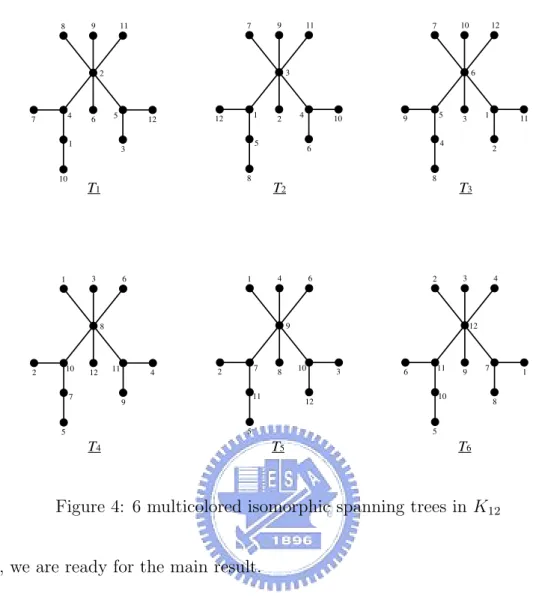
Lemma 2.1. The complete graph K12 admits an MTP.

Proof. Let V (K12) = {1, 2, · · · , 12} and the colors are C1, C2, · · · , C11. Let (i, j) be the

edge with endpoints i and j. Figure 3 and Figure 4 show the construction of an MTP of

K12.

T

1

T

2

T

3

T

4

T

5

T

6 C1: ( 2,11) ( 1,12) ( 5,12) ( 2, 8) ( 1,10) ( 4, 7) ( 2, 9) ( 3, 7) ( 4,10) ( 3,11) ( 3, 9) ( 5, 8) ( 5, 7) ( 6, 8) ( 1, 8) ( 4,11) ( 3, 8) ( 4, 8) ( 1,11) ( 5, 9) ( 6,10) ( 6,12) ( 6, 7) ( 2,10) ( 6, 9) ( 2, 7) ( 5,11) ( 3,10) ( 4, 9) ( 6,11) ( 3,12) ( 4,12) ( 2,12) ( 1, 7) ( 5,10) ( 1, 9) ( 3, 5) ( 1, 4) ( 2, 6) ( 2, 5) ( 2, 4) ( 2, 3) ( 1, 3) ( 3, 4) ( 1, 5) ( 4, 6) ( 5, 6) ( 4, 5) ( 1, 6) ( 3, 6) ( 1, 2) (11,12) (10,11) ( 7,12) ( 9,12) ( 7, 8) ( 8, 9) ( 7, 9) ( 9,10) ( 7,11) (10,12) ( 7,10) ( 8,12) ( 8,11) ( 8,10) ( 9,11) C2: C3: C7: C6: C5: C4: C11: C10: C9: C8: Figure 3: MTP of K12

9 11 8 2 6 5 4 ₁₂ 3 1 10 7 9 11 7 3 2 4 1 ₁₀ 6 5 8 12 10 12 7 6 3 1 5 ₁₁ 2 4 8 9 3 6 1 8 12 11 10 ₄ 9 7 5 2 4 6 1 9 8 10 7 ₃ 12 11 5 2 3 4 2 12 9 7 11 ₁ 8 10 5 6 T1 T6 T5 T4 T3 T2

Figure 4: 6 multicolored isomorphic spanning trees in K12

Now, we are ready for the main result.

Theorem 2.2. For m 6= 2, K2m admits an MTP.

Proof. By Theorem 1.8, it suffices to prove that if m is an odd integer, then K2madmits

an MTP.

Let K2m be defined on the set A ∪ B where A = {ai | i ∈ Zm} and B = {bi | i ∈ Zm}.

For convenience, let G1 =< A > and G2 =< B >. Since m is odd, by Theorem 1.2, G1

has a total coloring π which uses m colors, 1, 2, · · · , m. Now, define an edge-coloring ϕ of

K2m as follows:

(a) For each edge ajak ∈ E(G1), let ϕ(ajak) = π(ajak);

(b) For each edge bjbk ∈ E(G2), let ϕ(bjbk) = π(ajak);

(c) For each edge aibi, i ∈ Zm, let ϕ(aibi) = π(ai); and

(d) For each edge ajbk, j 6= k, let ϕ(ajbk) = m + t where t ≡ k − j (mod m) and

Clearly, ϕ is a (2m − 1)-edge-coloring of K2m. It is left to decompose K2m into m

multicolored isomorphic spanning trees. First, for each i ∈ {1, 2, 3, · · · , m}, let Ti be

defined on the set A ∪ B and E(Ti) = {aiai+2t (mod m), bibi+2t−1 (mod m), biai+2t−1 (mod m),

ai+1bi+2t (mod m) | t = 1, 2, · · · ,m−1₂ } ∪ {aibi}. Then, it is easy to check that Ti is a

span-ning tree of K2mand also Tiis multicolored. Furthermore, Tiand Tjare isomorphic follows

by the permutation of A ∪ B defined by mapping ai into aj and bi into bj respectively.

Now, if m is not an odd integer, then 2m = 2t_{· m}0 _{and t ≥ 2. In case that m}0 _{= 1,}

t must be at least 3. Then it is direct consequence of Theorem 1.8. On the other hand, m0 _{≥ 3. Thus K}

2t_m0 admits an MTP by using doubling construction obtained in [5] except

when m0 _{= 3 and t = 2. Since this case can be handled by Lemma 2.1, we conclude the}

proof.

We note here that the above theorem proves the weaker conjecture of Constantine and the result has been included in a paper written jointly with S. Akbari, A. Alipour and H. L. Fu [1] which is to appear in SIAM J. of Discrete Math.

2.2

Existence of Multicolored Hamiltonian Cycle Parallelism

To extend the study of parallelism to the other graph, K2m+1 deserves to be considered

first. Since χ0_(K

2m+1) = 2m + 1, the multicolored subgraph we consider has 2m + 1

edges. Thus, a multicolored Hamiltonian cycle in K2m+1 is the best candidate for the

subgraphs. In this section, we shall prove that for each positive integer m, there exists a

(2m+1)-edge-coloring of K2m+1 for which all edges can be partitioned into multicolored

Hamiltonian cycles. Obviously, any two Hamiltonian cycles are isomorphic and therefore we have another parallelism if exists.

Definition 2.3. We call K2m+1 admits a multicolored Hamiltonian cycle parallelism

(MHCP ) if there exists a (2m+1)-edge-coloring of K2m+1 for which all edges can be

partitioned into m multicolored Hamiltonian cycles.

For the convenience in the proof of our main result, we need a special circulant latin square M.

Definition 2.4. M = [mi,j] is a circulant latin square of order odd n with 1st row

(1,n+3 2 , 2, n+5 2 , 3, · · · , n+n 2 , n+1 2 ).

Figure 5 shows M of order 7.

Figure 5: Circulant latin square of order 7

Using M, we have a proper n-edge-coloring of Kn,n where {u1, u2, · · · , un} and {v1, v2,

· · · , vn} are the two partite sets of Kn,n. This coloring has an extra property that for 1 ≤

j ≤ n, the edges in {u1vj, u2vj+1, u3vj+2, · · · , unvj+n−1} form a perfect matching and they

We note here that if we permute the entries of M, we obtain another n-edge-coloring

of Kn,n which has the same property as above.

In order to prove the main theorem, we also need the following lemma.

Lemma 2.5. Let v be a composite odd integer and n is the smallest prime which is a

factor of v, say v = mn. Then Km(n) has an mn-edge-coloring such that the edge-colored

Km(n) can be partitioned into n(m−1)₂ multicolored Hamiltonian cycles if Km admits an

MHCP.

Proof. We prove the lemma by giving an mn-edge-coloring ϕ. Since Km defined on

{xi | i ∈ Zm} admits an MHCP , let µ be such an edge-coloring using the colors

0, 1, · · · , m − 1. Let V (Km(n)) =

m−1_[

i=0

Vi where Vi = {xi,j | j ∈ Zn} and L = [lh,k] be

a circulant latin square of order n as defined before Figure 5. Now, we have an

mn-edge-coloring of Km(n) by letting ϕ(xa,bxc,d) = lb,d+ µ(xaxc) · n. Therefore, the edges in Km(n)

joining a vertex of Va to a vertex of Vc, denoted (Va, Vc), are colored with the entries in

L + µ(xaxc) · n. It is not difficult to see that ϕ is a proper coloring of Km(n). Now, it

is left to show that the edges of Km(n) can be partitioned into multicolored Hamiltonian

cycles.

Let C = (c0, c1, c2, · · · , cm−1) = (xα(0), xα(1), · · · , xα(m−1)) (α is a permutation of Zm)

be a multicolored Hamiltonian cycle in Km obtained from the MHCP of Km. Define

Cm(n) to be the subgraph induced by the set of edges in

m−1_[

i=0

(Vα(i), Vα(i+1)). Now, if we let S(r0, r1, · · · , rm−1) be the set of perfect matchings in (Vα(0), Vα(1)), (Vα(1), Vα(2)),· · ·, (Vα(m−2), Vα(m−1)) and (Vα(m−1), Vα(0)) respectively where the perfect matching in (Vα(i),

Vα(i+1)), i = 0, 1, 2, · · · , m − 1, is the set of edges xα(i),axα(i+1),b with b − a ≡ ri (mod n),

ri ∈ Zn, then S(r0, r1, · · · , rm−1) is a 2-factor of Cm(n). Moreover, by the edge-coloring

we use for Km(n), S(r0, r1, · · · , rm−1) is indeed a multicolored 2-factor. Hence, we can

partition the edges of Cm(n) into n multicolored 2-factors due to the fact that ri ∈ Zn.

Note that S(r0, r1, · · · , rm−1) and S(r00, r01, · · · , rm−10 ) are edge-disjoint 2-factors if and only if ri 6= ri0 for each i ∈ Zm.

2-factor S(r0, r1, · · · , rm−1) is a Hamiltonian cycle. Observe that if m−1 X i=0

ri is not a multiple

of n, then S(r0, r1, · · · , rm−1) is a Hamiltonian cycle. (n is a prime.) Therefore, we let

(0, 0, · · · , 0, 1), (1, 1, · · · , 1, 2), · · · , and (n−1, n−1, · · · , n−1, 0) be the n m-tuples we need provided that n is not a factor of m · i + 1 for i = 0, 1, 2, · · · , n − 1. On the other hand,

assume that n | m · j + 1 for some j ∈ Zn.(Here, note that such j occurs at most once.)

If j ∈ {1, 2, · · · , n − 2}, then replace (j, j, · · · , j, j + 1) and (j + 1, j + 1, · · · , j + 1, j + 2) with (j, j, · · · , j, j + 1, j + 1) and (j + 1, j + 1, · · · , j + 1, j, j + 2) respectively. Otherwise, if

j = n−1, then replace (n−2, n−2, · · · , n−2, n−2, n−1) and (n−1, n−1, · · · , n−1, n−1, 0)

with (n − 2, n − 2, · · · , n − 1, n − 1, n − 1) and (n − 1, n − 1, · · · , n − 2, n − 2, 0) respectively.

This implies that in either case, we have a partition of the edges of Cm(n) into n

edge-disjoint multicolored Hamiltonian cycles. Moreover, since Km(n) can be partitioned into

m−1

2 Cm(n)’s, by a similar argument, we have a partition of the edges of Km(n)into m−12 · n

multicolored Hamiltonian cycles.

As an example, if m = n = 3, then the three multicolored Hamiltonian cycles are S(0, 0, 1) = (x0,0, x1,0, x2,0, x0,1, x1,1, x2,1, x0,2, x1,2, x2,2), S(1, 1, 2) = (x0,0, x1,1, x2,2, x0,1, x1,2, x2,0, x0,2, x1,0, x2,1), S(2, 2, 0) = (x0,0, x1,2, x2,1, x0,2, x1,1, x2,0, x0,1, x1,0, x2,2). In

case that m = 5 and n = 3, then we have 6 multicolored Hamiltonian cycles. For each

C5(3), we have three multicolored Hamiltonian cycles of type S(0, 0, 0, 0, 1), S(1, 1, 1, 2, 2),

and S(2, 2, 2, 1, 0).

Now, in order to partition the edges of an 9-edge-colored K9 into 4 Hamiltonian cycles,

we combine S(0, 0, 1) with the three cliques (K3) induced by the three partite sets V1, V2

and V3, to obtain a 4-factor. Since these K3’s can be edge-colored with {4, 5, 6}, {7, 8, 9}

and {1, 2, 3} respectively, we have an edge-colored 4-factor with each color occurs exactly twice. Thus, if this 4-factor can be partitioned into two multicolored Hamiltonian cycles,

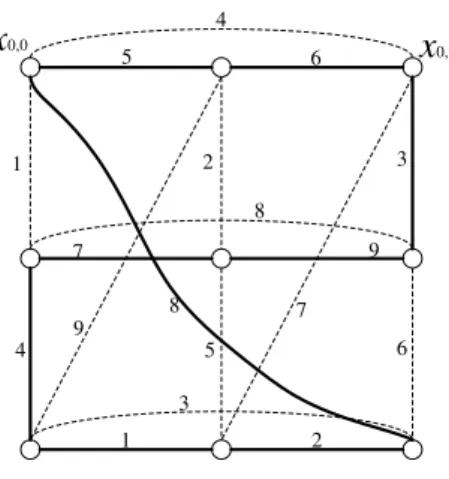
then we conclude that K9 admits an MHCP . Figure 6 shows how this can be done.

Notice that in the induced subgraphs < V1 >, < V2 > and < V3 > we have exactly

one edge from each graph which is not included in the cycle with solid edges. Therefore,

1 2 3 4 9 5 6 8 7 5 6 4 7 8 9 1 2 3 x0,0 x_0,2

Figure 6: Two multicolored Hamiltonian cycles of K9

the colors in (V1, V2), (V2, V3) and (V3, V1) respectively in order to obtain a multicolored

Hamiltonian cycle. For example, if the color of x0,0x0,2 is 5 instead of 4, then we permute

the entries in 46 65 54

5 4 6

by using (4,5), and thus the latin square used to color (V2, V3)

becomes 56 64 45

4 5 6

. This is an essential trick we shall use when n is a larger prime.

Theorem 2.6. For each odd integer v ≥ 3, Kv admits an MHCP.

Proof. The proof is by induction on v. By Theorem 1.12, the assertion is true for v is a prime. Therefore, we assume that v is a composite odd integer and the assertion is true for

each odd order u < v. Let n be the smallest prime such that v = n · m and V (Kv) =

m [ i=1

Vi

where Vi = {xi,j | j ∈ Zn}, i ∈ Zm. By induction, Km admits an MHCP and hence Km(n)

can be partitioned into m−1

2 Cm(n)’s each admits MHCP . Moreover, by Lemma 2.5, each

MHCP of Cm(n) contains a multicolored Hamiltonian cycle S(0, 0, · · · , 0, 1). Here, the

edge-coloring of Km(n) is induced by the coloring ϕ of Km, i.e., if vivj is an edge of Km

with color ϕ(vivj) = t ∈ Zm, then the colors of the edges in (Vi, Vj) are assigned by using

M + tn where M is a circulant latin square of order n as defined before Figure 5. We note

here again that permuting the entries of a latin square M + tn may give another coloring, but the coloring is still a proper coloring.

So, in order to obtain an MHCP of Kv, we first give a v-edge-coloring of Kv and

then adjust the coloring if it is necessary. Since Km(n) has an mn-edge-coloring ϕ, the

1, 2, · · · , m, where ψi is an n-edge-coloring of Knsuch that Kncan be partitioned into n−1₂

multicolored Hamiltonian cycles. Moreover, the images of ψi are 1 + tn, 2 + tn, · · · , n + tn

where t ∈ Zm and t is a color not occurs in the edges incident to vi ∈ V (Km). (Here, the

colors used to color the edges of Km are 0, 1, 2, · · · , m − 1.)

It is not difficult to check now µ is a v-edge-coloring of Kv. We shall revise µ by

permuting the colors in (Vi, Vi+1) for some i and finally obtain the edge-coloring we need.

For convenience, let the edges of Km(n) be partitioned into C_m(n)(1) , C_m(n)(2) , · · · , C

(m−1

2 )

m(n)

each contains a multicolored Hamiltonian cycle E(1)_{, E}(2)_{, · · · , E}(m−1

2 )of type S(0, 0, · · · , 0, 1)

and the edges of each Kn induced by Vi, i = 1, 2, · · · , m, be partitioned into n−1₂

multi-colored Hamiltonian cycles D(1)_{, D}(2)_{, · · · , D}(n−1₂ )_{. Since m ≥ n, we consider the 4-factors}

E(i)_{∪ D}(i) _{where i = 1, 2, · · · ,}n−1

2 . Starting from i = 1, we shall partition the edges of

E(1) _{∪ D}(1) _{into two Hamiltonian cycles such that both of them are multicolored. By}

the idea explained in Figure 6, we first obtain two Hamiltonian cycles from E(1)_{∪ D}(1)

by a similar way, see Figure 7 for example. For the purpose of obtaining multicolored

Hamiltonian cycles, we adjust the colors by permuting the colors in (Vi, Vi+1) to make

sure the first cycle does contain each color exactly once. Then, the second one is clearly

multicolored. Now, following the same process, we partition the edges of E(2)_{∪ D}(2)_{, · · ·,}

and E(n−1₂ )_{∪ D}(n−1₂ ) _{into two multicolored Hamiltonian cycles respectively. We remark}

here that if permuting entries of a latin square is necessary, then we can keep doing the same trick since C_m(n)(1) , C_m(n)(2) , · · · , C(m−12 )

m(n) are edge-disjoint subgraphs of Km(n). (The

per-mutations are carried out independently.) This concludes that after all the perper-mutations

are done, we obtain a v-edge-coloring of Kv such that Kv can be partitioned into v−1₂

multicolored Hamiltonian cycles.

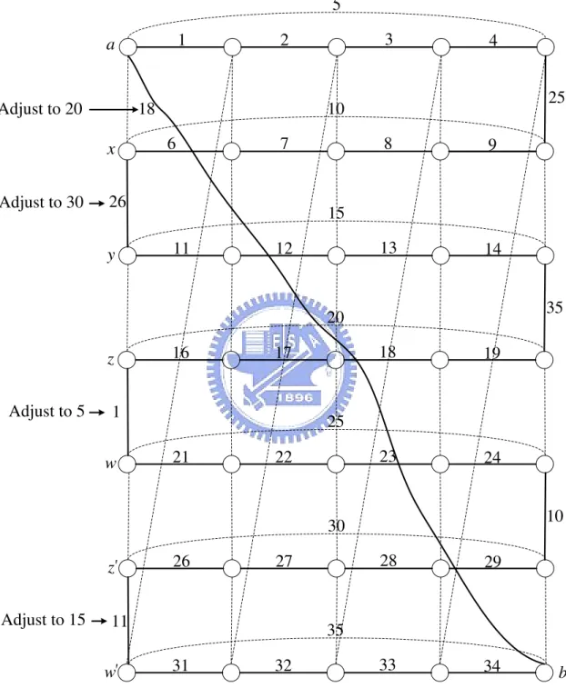
As a conclusion, we use Figure 7 to explain how our idea works. The edge xy was colored with 26 originally by using the circulant latin square of order 5 mentioned before Figure 5. But, 26 occurs in the Hamiltonian cycle with solid edges already. Therefore, we use (26, 30) to permute the square to obtain the edge-coloring we would like to have. After

adjusting the colors of zw, z0_w0 _{and ab respectively, we have two multicolored Hamiltonian}

1 2 3 4 5 8 9 10 11 12 13 14 15 16 17 18 19 20 21 22 23 24 25 26 27 28 29 30 31 32 33 34 35 25 26 35 10 1 11 Adjust to 30 Adjust to 5 Adjust to 15 x y z w z w ` ` 7 6 18 Adjust to 20 a b

3

The Existence of Multicolored (Rainbow) Subgraphs

3.1

Multicolored spanning trees in K

2m

Now, we consider a special edge-coloring of K2m with 2m − 1 colors such that for any

two colors form an C4-factor. Let L be the 2-group latin square defined earlier in Section

1.2. In what follows, we show that Ln _{= L × L × · · · × L based on Z}

2n has 2n disjoint

transversals for each n ≥ 2.

Proposition 3.1. Ln _{has 2}n _{disjoint transversals for each n ≥ 2.}

Proof. The proof is by induction on n and by Figure 2, n = 2 is true.

0 1 2 3 0 0 0 0 0 0 0 0 3 1 1 1 1 1 1 1 1 2 2 2 2 2 2 2 2 3 3 3 3 3 3 3 (0,1) (0,0) (1,0) (0,0) (0,0) (0,0) (0,1) (0,1) (0,1) (1,1) (1,0) (1,0) (1,0) (1,1) (1,1) (1,1) (0,0) (0,1) (1,0) (0,0) (0,0) (0,0) (0,1) (0,1) (0,1) (1,1) (1,0) (1,0) (1,0) (1,1) (1,1) (1,1) (0,0) (0,1) (1,0) (0,0) (0,0) (0,0) (0,1) (0,1) (0,1) (1,1) (1,0) (1,0) (1,0) (1,1) (1,1) (1,1) (0,0) (0,1) (1,0) (0,0) (0,0) (0,0) (0,1) (0,1) (0,1) (1,1) (1,0) (1,0) (1,0) (1,1) (1,1) (1,1) Figure 8: 4 transversals in L2

Assume that the assertion is true for each k ≥ 2. Let Lk _{= [l}

a,b(k)] and Lk+1 =

L0k L1k

L1k L0k . By definition of direct product, we have L0

k _{= [m}

a,b] where ma,b =

(0 , la,b(k)) (a (k+1)-dim. vector) and L1k = [ma,b] where ma,b = (1 , la,b(k)). We

shall use the set of 2k _{disjoint transversals in L}k _{to construct 2}k+1 _{disjoint transversals in}

Lk+1_.

Let {Ai | i = 0, 1, 2, · · · , 2k− 1} be the set of disjoint transversals obtained in Lk by

induction hypothesis. W.L.O.G. we may let Ai be the transversal which contains the entry

l0,i(k), i = 0, 1, 2, · · · , 2k− 1. Now, we shall use A2i and A2i+1, i = 0, 1, 2, · · · , 2k−1− 1, to

construct four disjoint transversals in Lk+1_{. For convenience, we explain the construction}

by using A0 and A1.

Since A0(respectively A1) is a transversal in Lk, the corresponding entries in L0kform

of A0 in L0k and L1k be A0,0 and A1,0 respectively. Similarly, let the corresponding

transversals of A1 be A0,1 and A1,1 respectively. Note that for 0 ≤ r, s ≤ 1, Ar,s has 2k

entries one from each row and from each column. Now, for 0 ≤ r, s ≤ 1, we split Ar,s into

two parts: Ar,s

(u)

is the set of entries from the first to the 2k−1_{-th row of A}

r,s, and Ar,s

(l)

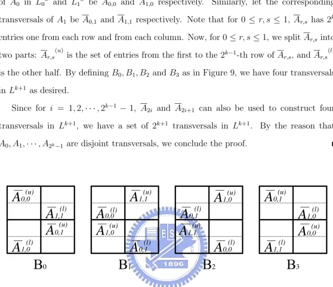
is the other half. By defining B0, B1, B2 and B3 as in Figure 9, we have four transversals

in Lk+1 _{as desired.}

Since for i = 1, 2, · · · , 2k−1 _{− 1, A}

2i and A2i+1 can also be used to construct four

transversals in Lk+1_{, we have a set of 2}k+1 _{transversals in L}k+1_{. By the reason that}

A0, A1, · · · , A2k₋₁ are disjoint transversals, we conclude the proof.

A

0,1 (u)

A

0,0 (u)

A

1,0 (u)

A

1,0 (u)

A

0,0 (u)

A

1,0 (l)

A

0,0 (l)

A

0,0 (l)

A

1,0 (l)

A

1,1 (l)

A

0,1 (l)

A

0,1 (l)

A

1,1 (l)

A

0,1 (u)

A

1,1 (u)

A

1,1 (u) 0 1 2 3

Figure 9: 4 transversals in Lk+1 _{constructed from A}

0 and A1

Lemma 3.2. Let µ be a (2m − 1)-edge-coloring of K2m, m ≥ 2, such that for any two

colors induce a 2-factor with each component a 4-cycle, then (a) 2m = 2n _{for some n ≥ 2}

and (b) K2m contains a clique K of order 2k, 1 ≤ k ≤ n − 1 such that {µ(e) | e ∈ E(K)} is a (2k_{− 1)-set, i.e., µ|}

K is a (2

k_{− 1)-edge-coloring of K.}

Proof. First, we claim that (b) is true. The proof is by induction on n. Clearly, it is

true when n = 2. By hypothesis, let H be a clique of order 2h_{, h < k, and µ|}

H is a

(2h _{− 1)-edge-coloring of H. W.L.O.G. let V (H) = {x}

1, x2, · · · , x2h} and the colors used

in H be {c1, c2, · · · , c2h₋₁}. Since µ is a (2m−1)-edge-coloring of K_2m, each color occurs

around each vertex. Let c₂h be a color not used in H. Then, we have a set H0, H0∩H = φ,

H0 _{= {y}

any two colors induce a C4-factor, we conclude that µ|H0 is also a (2

h_{− 1)-edge-coloring}

of H0_{, moreover, µ(x}

ixj) = µ(yiyj) for 1 ≤ i 6= j ≤ 2h. Therefore, the complete bipartite

graph K₂h_,2h = (H, H0) has a 2h-edge-coloring following by the same reason. This implies

that µ|_H∪H0 is a (2h+1_{− 1)-edge-coloring of the clique induced by H ∪ H}0_{. So, we have the}

proof of (b).

Suppose 2m = 2r_{· p where p is an odd integer and p 6= 1. Using above argument,}

we can find the biggest clique G of order 2s _{which uses 2}s_{− 1 colors. Then we partition}

the vertices of K2m into two sets X and Y where X = V (G), and let |Y | = q. Here, we

notice that q < 2s_{. Consider these 2}s_{− 1 colors used in coloring the edges of G, in total,}

there are (2s_{− 1)(2}r−1_{· p) edges which use these colors. But, we have used these colors}

in G. Hence, there remains 2s−1₍₂s_{− 1)(}q

2 − 1) edges to be colored by using these colors.

Since the edges between X and Y can’t be colored with any of these colors, they have to

be in Y. But, since q < 2s_{, 2}s−1₍₂s_{− 1)(}q

2 − 1) >

¡_q

2

¢

, a contradiction. This implies that

p = 1, and we have the proof of (a).

Now, we are ready to prove the main result.

Theorem 3.3. Let µ be a (2m − 1)-edge-coloring of K2m, m > 2, such that for any two

colors induce a 2-factor with each component a 4-cycle. Then the edges of K2m can be partitioned into m isomorphic multicolored spanning trees.

Proof. By lemma 3.2, 2m = 2n _{for some n > 2. We prove the theorem by induction on}

n. By Lemma 1.10, n = 3 is true.

Assume that the assertion is true for each k ≥ 3 and consider K2k+1.

From the process of the proof of Lemma 3.2, it must exist two disjoint cliques of

order 2k _{with 2}k_{− 1 colors in K}

2k+1. Let V (K₂k+1) = A ∪ B where A, B are the vertex

sets of the two cliques. Consider the colors of the edges between A and B. Let A =

{a0, a1, . . . , a2k₋₁}, B = {b₀, b₁, . . . , b₂k₋₁}, and define an array M = [m_i,j] by µ(a_ib_j) =

mi,j. It’s clear that M is a latin square, furthermore, M ∼= Lk. By Proposition 3.1, M has

2k _{disjoint transversals. This implies that there are 2}k _{perfect matchings in the complete}

have 2k−1_{isomorphic spanning trees of order 2}k_{, respectively. Thus, by assigning a perfect}

matching to each spanning tree, we obtain 2k _{spanning trees of order 2}k+1_{. Moreover,}

these spanning trees are isomorphic and multicolored.

Now, we are ready to consider K2m with an arbitrary (2m − 1)-edge-coloring.

Theorem 3.4. Let ϕ be an arbitrary (2m-1)-edge-coloring of K2m. Then there exist two

isomorphic multicolored spanning trees in K2m for m ≥ 3.

Proof. Let V (K2m) = {xi| i ∈ Z2m}. We split the proof into two cases.

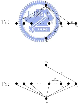
Case 1. There exists a 4-cycle (x0, x1, x2, x3) such that ϕ(x0x1) = b, ϕ(x2x3) = c, and

ϕ(x0x3) = ϕ(x1x2) = a. Then the two isomorphic multicolored spanning trees can

be obtained by the following figure.

x0 a x2 x3 x1 x1 x2 x3 x0 a b b . . . . . . . . . . 1 2

Figure 10: Two isomorphic spanning trees

Case 2. If any two colors of this edge-coloring induce a C4-decomposition of K2m, then

3.2

Multicolored unicyclic spanning subgraphs in K

2m+1

Since χ0_(K

2m+1) = 2m + 1, we consider K2m+1 with a proper (2m + 1)-edge-coloring.

Theorem 3.5. For any positive integer m, given an arbitrary proper (2m+1)-edge-coloring

of K2m+1, there exists a pair of multicolored isomorphic unicyclic spanning subgraphs of K2m+1.

Proof. For each (2m+1)-edge-coloring K2m+1, we observe that each vertex of K2m+1 is

missing one color (exactly) of the color-set Z2m+1, and each color of the color-set occurs

exactly m times. Therefore, if u and v are two distinct vertices, then their corresponding

missing colors are distinct. So, without loss of generality, we may let V (K2m+1) = Z2m+1,

and at vertex i ∈ Z2m+1, the color missing is i.

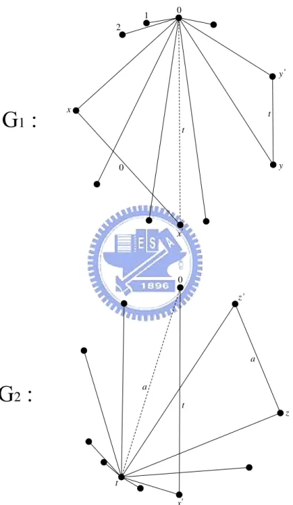
Now, we can construct two multicolored subgraphs. In the first graph, we use the star

with center 0 which has 2m edges. Then delete one edge 0x0 _{which is colored ”t” 6= 0.}

Let this star be H1. Now, by adding an edge yy0 (colored t) and an edge xx0 (colored 0),

we have the desired subgraph G1 = H1+ yy0+ xx0. The second graph can be obtained by

a similar way, which is from the star H2 with center t by deleting one edge 0t. Let 0t be

of color a. Then, adding an edge (different from 0t) of color a and the edge 0x’ we have

the desired second subgraph G2 = H2+ 0t + 0x0.

Clearly, these two graphs are multicolored and the unique cycle in them are both a triangle. Since they are spanning subgraphs, we have a pair of multicolored isomorphic

unicyclic spanning subgraphs of K2m+1.

1

2

0 1 2 x x y y` ` t t 0 0 t x ` t a a z z `

4

Conclusion

In this thesis, we have obtained the following four main results:

1. A multicolored tree parallelism for K2m, m ≥ 3.

2. A multicolored Hamiltonian cycle parallelism for K2m+1, m ≥ 2.

3. The existence of two isomorphic multicolored spanning trees in an (2m −

1)-edge-colored K2m.

4. The existence of two isomorphic multicolored unicyclic spanning subgraphs in an

(2m + 1)-edge-colored K2m+1.

From the results, we are able to prove the weaker conjecture (Conjecture 1.4) posed by Constantine. But, we are very far from verifying the other conjectures. Hopefully, this task can be done in the near future.

References

[1] S. Akbari, A. Alipour, H. L. Fu and Y. H. Lo, Multicolored parallelism of isomorphic spanning trees, SIAM Discrete Math., to appear.

[2] N. Alon, R. A. Brualdi and B. L. Shader, Multicolored forests in bipartite decompo-sition of graphs, J. Combin. Theory Ser. B, 53(1991) 143-148.

[3] R. A. Brualdi and S. Hollingsworth, Multicolored trees in complete graphs, J. Com-bin. Theory Ser. B, 68(1996), No. 2, pp. 310-313.

[4] P. J. Cameron, Parallelisms of complete designs, London Math. Soc. Lecture Notes Series, 23(1976), Cambrideg University Press.

[5] G. M. Constantine, Multicolored parallelisms of isomorphic spanning trees, Discrete Math. Theor. Comput. Sci. 5(2002), No. 1, 121-125.

[6] G. M. Constantine, Edge-disjoint isomorphic multicolored trees and cycles in com-plete graphs, SIAM Discrete Math. 18(2005), No. 3, 577-580.

[7] J. Krussel, S. Marshal and H. Verral, Spanning Trees Orthogonal to

One-Factorizations of K2n, Ars Combin. 57(2002), 77-82.

[8] D. B. West(2001), Introduction to graph theory, Upper Saddle River, NJ :Prentice Hall.

[9] D. E. Woolbright and H. L. Fu, On the exists of rainbows in 1-factorizations of K2n,

J. Combin. Des. 6(1998), 1-20.

[10] H. P. Yap, Total colourings of graphs, Lecture Notes in Mathematics, 1623. Springer-Verlag, Berlin, 1996.