正規化最小平方法為基礎的階層式合作共同進化演算法及其於模糊類神經網路設計和影像對準的應用

國 立 交 通 大 學

電控工程研究所

博士論文

正規化最小平方法為基礎的階層式合作共同進化演

算法及其於模糊類神經網路設計和影像對準的應用

Regularized Least Squares based Hierarchical Cooperative

Coevolutionary Algorithm for Neural Fuzzy Network Design

正規化最小平方法為基礎的階層式合作共同進化演

算法及其於模糊類神經網路設計和影像對準的應用

Regularized Least Squares based Hierarchical Cooperative

Coevolutionary Algorithm for Neural Fuzzy Network Design

and Image Alignment Applications

研 究 生：徐啟曜

Student：Chi-Yao Hsu

指導教授：林昇甫 博士

Advisor：Dr. Sheng-Fuu Lin

國 立 交 通 大 學

電控工程研究所

博 士 論 文

A Dissertation

Submitted to Institute of Electrical Control Engineering

National Chiao-Tung University

In Partial Fulfillment of the Requirements

For the Degree of

Doctor of Philosophy

in

Electrical and Control Engineering

June 2012

Hsinchu, Taiwan, Republic of China

正規化最小平方法為基礎的階層式合作共同進化演

算法及其於模糊類神經網路設計和影像對準的應用

研究生：徐啟曜 指導教授：林昇甫 博士

國立交通大學 電控工程研究所

摘 要

進化型演算法經常被使用在訓練模糊類神經網路參數方面，主要是因為該方法有並 行搜尋的技術。不過目前此類型的方法有著無法拓展到多數量的訓練參數以及低效率的 調整模糊法則問題，所以本篇論文提出了正規化最小平方法為基礎的階層式合作共同進 化演算法來改善上述問題。使用正規化最小平方法的主要效用為減少訓練參數的數量， 而在階層式合作共同進化演算法方面，兩層級進化法被提出能夠有效地進化模糊規則以 及使得網路的參數及其架構能夠被分別被區域性及全域性的進化，因此以正規化最小平 方法為基礎的階層式合作共同進化演算法有著參數學習及架構學習的優點，並且進化完 成的網路可以被應用到現實世界的實例。第一個應用為二維影像對準問題，本論文所提 出的演算法則可用來建立一個以合作式模糊類神經網路為基礎的二維影像對準系統，該 系統利用多級模糊神經網路來解決單級模糊神經網路在仿射參數的大範圍應用的困 難。第二個應用為三維影像對準問題，採用本論文所提的學習演算法可建立以模糊類神

Regularized Least Squares based Hierarchical Cooperative

Coevolutionary Algorithm for Neural Fuzzy Network Design

and Image Alignment Applications

Student：Chi-Yao Hsu Advisor：Dr. Sheng-Fuu Lin

Institute of Electrical Control Engineering

National Chiao Tung University

Abstract

Evolutionary algorithms are very popular in training parameters of neural fuzzy network due to their parallel search techniques. However, current methods have problems of not scaling well to a large number of training parameters and adjusting fuzzy rules inefficiently. In this dissertation, a regularized least squares based hierarchical cooperative coevolutionary algorithm (RGLS-HCCA) is proposed to improve above problems. The major utility of RGLS is to reduce the number of learning parameters. In HCCA, two-level evolution is proposed to evolve fuzzy rules efficiently and make the parameters and structure of a network be evolved locally and globally, respectively. Thus, RGLS-HCCA has advantages of parameter learning and structure learning, and the evolved network can be applied to the real world applications. The first application is a 2D image alignment problem. The proposed RGLS-HCCA is used to construct a cooperative neural fuzzy network (CNFN)-based 2D image alignment system, which utilizes the multi-stage of neural fuzzy networks to solve problems that one-stage of neural network have difficulty in applying a large range of affine parameters. The second application is a 3D image alignment problem. The use of RGLS-HCCA can construct a neural fuzzy network (NFN)-based coarse-to-fine 3D image alignment system, which solve the problem of the high alignment error caused by principle component analysis (PCA) and heavy computational cost caused by iterative closest point (ICP). The evidence can be found in experimental results demonstrate the superior performance of the proposed 2D and 3D surface alignment system over typical systems.

Keywords: regularized least squares, hierarchical cooperative coevolutionary algorithm,

誌謝

經過多年的努力，終於取得博士學位，在博士班的研究生涯中，首先要感謝我的指 導教授-林昇甫博士，林教授在研究上給予學生正確方向的指導，讓學生覺得獲益良多， 並且林教授總是正向地鼓勵學生，讓學生對於學術研究充滿了信心，有了這份信心學生 才能夠通過論文投稿以及博士口試這兩大關卡，所以非常感謝林教授的指導。 在博士論文口試方面，感謝口試委員潘晴財教授、鍾鴻源教授、張翔教授及林錫寬 教授不辭辛苦參與學生的口試，並給與學生許多寶貴的修正意見，讓學生的論文能夠更 加地完整，所以學生由衷地感謝口試委員。 接下來要感謝 806 實驗室的博士班學長弦澤及培家、同學逸章、學弟俊偉及裕筆， 碩士班學弟柏宏、植彥、俊良、學妹婷婷及雅君，有了你們的幫忙，我的求學之路才會 如此順利，另外特別要感謝實驗室已畢業的博士班學長-徐永吉博士，有了你在論文上 的互相討論及協助，我才能完成博士論文中的許多研究。 也感謝中科院各個長官的栽培及支持，讓我能夠有機會攻讀博士，並順利取得博士 學位，而我的同事也在我的求學之路上幫忙很多，不論在工作上的協助，或是在研究上 的心得分享，對我而言都是相當大的助力。 而我的父母是我的心靈上的寄託，感謝你們對我的支持及鼓勵，我才能有信心接受 許多挑戰，並達成我人生重要的夢想-取得博士學位，而我的哥哥對我的照顧，我也是 心存感激。另外我要感謝我相識多年的女友，每當我在研究或工作上遇到挫折，妳總是 在我身邊陪我渡過許多的難關。 最後我要再次感謝所有幫過我的人，有了你們的幫忙，我才能夠取得博士學位。

Contents

Chinese Abstract ...ii

EnglishAbstract... iii

Chinese Acknowledgement ...iv

Contents...v

List of Tables ...vii

List of Figures ... viii

List of Figures ... viii

Chapter 1 Introduction ...1 1.1 Motivation ... 1 1.2 Related Works... 3 1.3 Approach ... 6 1.4 Organization of Dissertation ... 8 Chapter 2 Foundations...10

2.1 Regularized Least Squares Method ... 10

2.2 Neural Fuzzy Network ... 11

2.3 Cooperative Coevolutionary Learning ... 14

2.4 2D Image Alignment... 17

2.5 3D Image Alignment... 19

Chapter 3 Regularized Least Squares Based Hierarchical Cooperative ...24

Coevolutionary Algorithm...24

3.1 Parameter Level Evolution ... 25

3.2 Structure Level Evolution... 40

Chapter 4 Image Alignment Applications ...44

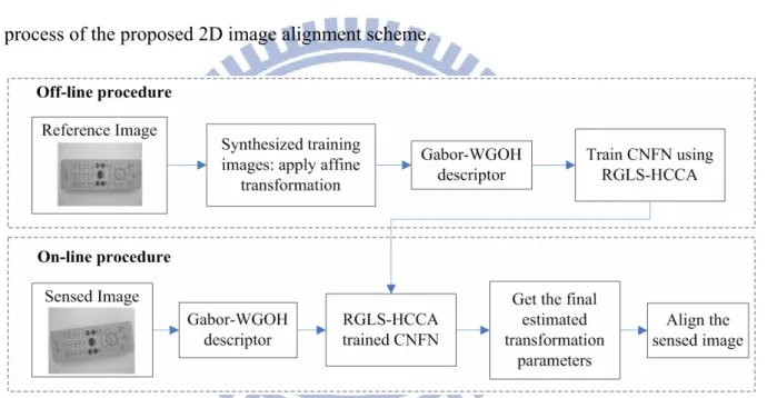
4.1 2D Image Alignment System ... 44

4.1.1 Off-line Procedure ... 45

4.1.2 On-line Procedure ... 50

4.2 3D Image Alignment System ... 50

4.2.1 Learning Phase ... 51

Chapter 5 Experimental Results ...63

5.1 Prediction of Mackey-Glass Time Series ... 63

5.2 Results of 2D Image Alignment ... 69

5.2.1 Alignment Results of One-stage Neural Fuzzy Network ... 70

5.2.2 Alignment Results of Multi-stage Neural Fuzzy Networks ... 79

5.3 Results of 3D Image Alignment ... 89

Chapter 6 Conclusions and Future Works ...95

6.1 Conclusions ... 95

6.2 Future Works ... 96

Bibliography...98

Vita ...109

List of Tables

Table 3.1: Transactions in the DMSM...34

Table 5.1: Initial parameters of RGLS-HCCA before training...64

Table 5.2: Initial parameters of four learning models. ...69

Table 5.3: Performance comparison of various existing models...69

Table 5.4: Comparison of the running time of various algorithms...69

Table 5.5: Experimental images preparation. ...71

Table 5.6: Range of affine transformation parameters used in experiments. ...71

Table 5.7: Initial parameters before training. ...72

Table 5.8: Leaning accuracy of the RGLS-HCCA, HESP, ESP, and SANE methods. ...73

Table 5.9: Alignment errors in different image alignment systems...74

Table 5.10: Target alignment range. ...80

Table 5.11: Affine parameters range of three-stage CNFNs...80

Table 5.12: Initial parameters of RGLS-HCCA training...81

Table 5.13: Alignment errors in different image alignment systems...83

Table 5.14: Range of 3D rigid transformation parameters. ...90

Table 5.15: Learning parameters for the TNFN training...91

List of Figures

Figure 2-1: Structure of TNFN. ...13

Figure 2-2: Basic Steps of SANE. ...15

Figure 2-3: Structure of the chromosome in MGCSE...16

Figure 2-4: Coding a fuzzy rule of a TNFN into a chromosome in MGCSE...17

Figure 2-5: Example of generating training images with different affine transformation: (a) reference image, (b) translation, (c) clockwise rotation, and (d) counterclockwise rotation...18

Figure 2-6: Typical procedure of an area-based 2D image alignment system. ...18

Figure 2-7: Example of 2D alignment: (a) reference image, (b) image with an affine transformed, and (c) alignment results of neural network based scheme...19

Figure 2-8: Example of 3D image. ...21

Figure 2-9: Procedure of a 3D surface alignment task ...21

Figure 2-10: Example of coarse alignment using PCA: (a) the principal axes of the reference model, (b) the principal axes of the input 3D data, and (c) alignment results of the PCA method...23

Figure 2-11: Example of fine alignment using ICP: (a) the initial alignment yielded by PCA and (b) alignment results of the ICP method. ...23

Figure 3-1: Learning process of RGLS-HCCA...25

Figure 3-2: Coding the probability vector to represent the suitability of a TNFN with Mk rules. ...26

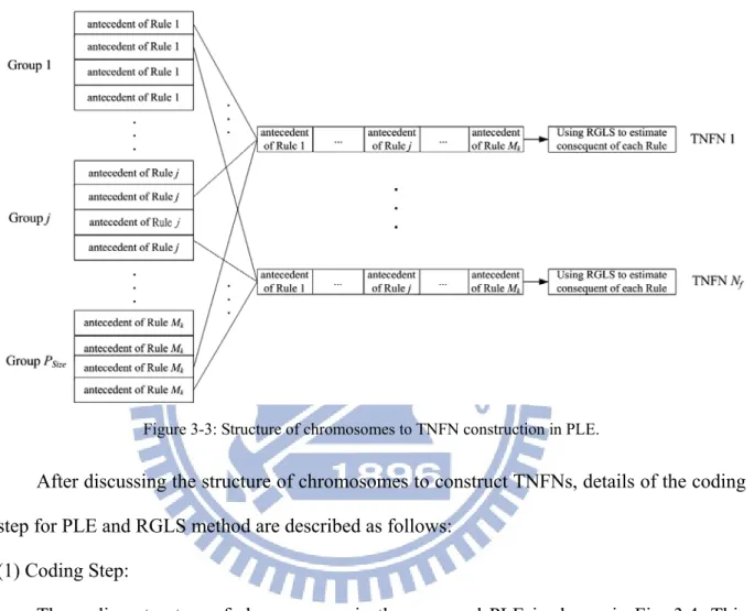
Figure 3-3: Structure of chromosomes to TNFN construction in PLE...27

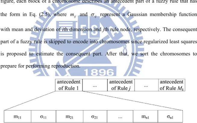
Figure 3-4: Coding an antecedent part of a fuzzy rule into a chromosome in PLE. ...28

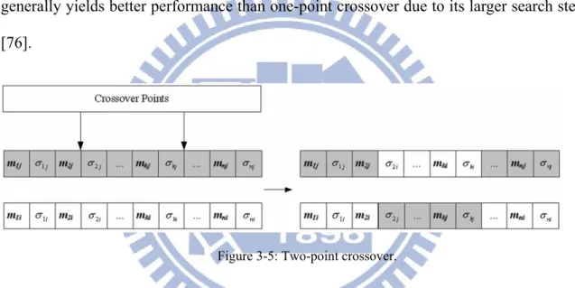
Figure 3-5: Two-point crossover. ...38

Figure 3-6: The learning process of PLE...39

Figure 3-7: The coding the antecedent part of fuzzy rules into a chromosome in the structure level evolution. ...40

Figure 4-7: Creation of viewpoint feature histogram. ...53

Figure 4-8: Example of similar viewpoint feature histograms in much different view...54

Figure 4-9: Diagram describes two viewpoint direction related angles θ and φ...55

Figure 4-10: Example of modified viewpoint feature histograms in much different view. ...56

Figure 4-11: Location of cube and reference model...58

Figure 5-1: Prediction results of the (a) proposed RGLS-HCCA, (b) HESP, (c) ESP, and (d) SANE...66

Figure 5-2: Prediction errors of the (a) proposed RGLS-HCCA, (b) HESP, (c) ESP, and (d) SANE...67

Figure 5-3: Learning curves of the proposed RGLS-HCCA, HESP, ESP, and SANE...67

Figure 5-4: (a) Reference image. (b) Testing image with scale=0.9, rotation=-10°, vertical translation=5, horizontal translation=10...70

Figure 5-5: Best results of the probability vectors for 15 runs in SRM. ...73

Figure 5-6: Learning curves of the RGLS-HCCA, HESP, ESP, and SANE methods...73

Figure 5-7: Alignment results for different systems: (a) Ground Truth, (b) OS-CNFN, (c) DCT, (d) FFT, (e) KICA, (f) ISOMAP, and (g) SIFT. ...75

Figure 5-8: Alignment results for different systems under 10 dB SNR condition: (a) Ground Truth, (b) OS-CNFN, (c) DCT, (d) FFT, (e) KICA, (f) ISOMAP, and (g) SIFT. ...77

Figure 5-9: Average affine transformation errors comparison using OS-CNFN, DCT, FFT, KICA, ISOMAP, and SIFT under various SNR. Error with respect to (a) scale, (b) rotation, (c) translation on X-axis, and (d) translation on Y-axis. ...78

Figure 5-10: Results of image alignment on real images: (a) OS-CNFN, (b) DCT, (c) FFT, (d) KICA, (e) ISOMAP, (f) SIFT. ...79

Figure 5-11: Recursive training curve of performing self-organized training data yielding method: (a) Coarse range, (b) Medium range, and (c) Fine range. ...81

Figure 5-12: Alignment results for different systems: (a) Ground Truth, (b) MS-CNFN, (c) DCT, (d) FFT, (e) KICA, and (f) ISOMAP...83

Figure 5-13: Average affine transformation errors comparison using MS-CNFN, DCT, FFT, KICA, ISOMAP under various SNR. Errors with respect to (a) scale, (b) rotation, (c) translation on X-axis, and (d) translation on Y-axis...85

Figure 5-14: Alignment results for different systems under 10 dB SNR condition: (a) Ground Truth, (b) MS-CNFN, (c) DCT, (d) FFT, (e) KICA, and (f) ISOMAP...86

Figure 5-15: Alignment results for different systems under salt and pepper noise: (a) Ground Truth, (b) MS-CNFN, (c) DCT, (d) FFT, (e) KICA, and (f) ISOMAP...87

Figure 5-16: Results of image alignment on real images: (a) MS-CNFN, (b) DCT, (c) FFT, (d) KICA, and (e) ISOMAP. ...88

Figure 5-17: Results of image alignment on circuit board inspection images: (a) the template, (b) without rotation, (c) counterclockwise rotation, (d) clockwise rotation, (e) counterclockwise rotation, and (f) clockwise rotation...89

Figure 5-18: Examples of two coarse alignment methods: (a) PCA and (b) TNFN-based coarse alignment...92 Figure 5-19: Real case of 3D point cloud data scanned by a 3D imaging laser scanner...93 Figure 5-20: Coarse alignment results: (a) PCA and (b) TNFN-based coarse alignment. ...93 Figure 5-21: Fine alignment results: (a) TNFN-based fine alignment, (b) NNM, and (c) ICP.94

Chapter 1

Introduction

For most interesting real world problems, the environment is more complicated and highly non-linear. For instance, to consider image alignment problems, the prediction of the relationship between input image and output pose is non-linear and it is hard to use the linear mathematical tools to accomplish modeling. Based on this fact, neural fuzzy networks can take its “black box” nature and linguistic information to deal with non-linearity. Thus, the purpose of this dissertation is to develop a methodology to automatically design neural fuzzy networks by using regularized least squares (RGLS) based hierarchical cooperative coevolutionary algorithm (HCCA) to evolve the networks for applying to real world problems.

This chapter is divided into four subsections. In Section 1.1, the motivation of this dissertation is introduced. Section 1.2 describes the related works of the evolutionary algorithm and image alignment applications. Section 1.3 specifies the proposed approach. In Section 1.4 the organization of this dissertation is presented.

1.1 Motivation

In most physical systems, the relationship between input and output is inherent non-linear in nature. Non-linear relationship is difficult to solve and give rise to interesting research topics. To cope with non-linearity, neural networks are algorithms that can be used to perform nonlinear statistical modeling and diverse engineering applications based on this modeling method have been successfully developed. However, their operation is restricted to the numeric domain. In recent years, neural fuzzy networks (NFNs) used for several problems have become a popular research topic [1]-[6], especially for solving nonlinear and complex problems [7]-[10]. The reason is that it combines fuzzy set and fuzzy logic into the neural

network framework to bring the benefits of processing linguistic and numeric information. Training parameters is the main issue for designing neural fuzzy networks. The most well known algorithm is back-propagation (BP) [3], [6] which is a powerful training technique for tuning the parameters of networks. Since the BP algorithm adopts the steepest decent approach to minimize the error function, they suffer from a major problem: getting in local minima of the error surface. To deal with the drawback, there is a need to face with suboptimal problem. Towards this end, evolutionary algorithms appear to be better candidates than the BP algorithm because of their parallel search techniques and optimization methodology.

Recently, several evolutionary algorithms, including genetic algorithm (GA) [11], hierarchical genetic algorithm (HGA) [12], symbiotic adaptive neruoevolution (SANE) [13], enforced sub-population (ESP) algorithm [14], and multi-groups cooperation based symbiotic evolution (MGCSE) [15] have been proposed to train neural networks or fuzzy systems. Although these algorithms can obtain better performance than the BP algorithm, they still have difficulty in scaling to more complex tasks or high input dimension of networks. Moreover, they also conduct the problem of the random group selection of fuzzy rules and the lost of potential fuzzy rules combinations. Therefore, these problems are the main issues this dissertation intends to address.

Furthermore, to transfer the problem from simulation to the real world applications, two image alignments tasks are utilized. The first one is a 2D image alignment problem which is

1.2 Related Works

Neural fuzzy networks are gaining research interest and they have been widely used in fields of pattern recognition, control problems, image processing, and diagnosis. The major benefit of neural fuzzy network is the integration of computation power from neural networks and human-like reasoning from fuzzy systems. Since neural fuzzy networks can bring such benefit, how to train neural fuzzy networks has become a critical issue.

The back-propagation (BP) algorithm [3] is a typical method for training neural fuzzy networks. Although the use of steepest descent technique in BP learning can reach the local minimal much quickly, the global minimal may be never found. Thus, evolutionary algorithms are better ones than BP due to their parallel search techniques. Recently, evolutionary fuzzy models have become a popular research field [16]-[24]. The evolutionary fuzzy model is a learning process using evolutionary learning procedures to generate a fuzzy system automatically. Among these evolutionary fuzzy models, the well-known algorithms are the genetic fuzzy models, which are augmented by incorporating genetic algorithms (GAs). There are several genetic fuzzy models have been proposed [16]-[18]. In [16], Karr adopted GAs to adjust membership functions for designing a fuzzy controller where its fuzzy rule set must be predetermined. Lin and Jou [17] applied GAs to fuzzy reinforcement learning to control a magnetic bearing system. In [18], Juang et al. proposed symbiotic evolution based genetic reinforcement learning for designing fuzzy controllers. In their work, the symbiotic-evolution-based fuzzy controller required fewer trail and less CPU time than the traditional GA-based fuzzy controller.

Although the genetic fuzzy models can be used to search for the optimal solution, they may have some limitations, such as the same lengths of chromosomes, predefined parameters, and so on. Thus, there are several improved evolutionary algorithms [19]-[22] to take into account these limitations. In [19], Carse et al. used the fusion of genetic algorithms and fuzzy

logic to evolve variable length fuzzy rule-sets. In [20], Bandyopadhyay et al. proposed variable-length genetic algorithm (VGA) to encode different length of chromosomes in the same population. Tang [21] proposed a hierarchical genetic algorithm to enable the optimization of designing a fuzzy system for particular applications. Juang [22] proposed a combination of online clustering and Q-value based GA learning for fuzzy system design (CQGAF) to generate fuzzy rules automatically and free parameters in a fuzzy system. In addition, Gomez and Schmidhuber [14] proposed enforced subpopulations (ESP) to provide several subpopulations to evaluate each partial solution. The subpopulations that are used to evaluate the solution locally can obtain better performance than those methods that only use one population for evaluating the solution. In [15], Hsu and Lin proposed a multi-groups cooperation based symbiotic evolution (MGCSE) to train a TSK-type neuro-fuzzy network (TNFN). They develop a novel symbiotic evolution to let each sub population can cooperate to generate better offspring.

In spite of the above evolutionary learning algorithms improving genetic fuzzy models, these algorithms may conduct one or more of the following problems: (1) the random group selection of fuzzy rules, (2) low convergence rate as the problem becomes complex, and (3) potential fuzzy rules combinations are lost.

Recently, hierarchical enforced sub-populations (HESP) [23] provided a hierarchical evolutionary for preserving the potential neuron combinations. In their work, in spite of keeping useful networks, HESP still suffer from: the lengths of chromosomes must be the

the number of fuzzy rules automatically.

In addition, to consider 2D image alignment application, the problem of precise image alignment has been well-studied in several fields. In [30], Liu et al. point out that image alignment techniques are broadly classified as feature-based[31] and [32] and area-based matching approaches[33-35]. Amintoosi et al. pointed out that area-based methods produce better results than results with low signal-to-noise ratio (SNR) from feature-based methods. Moreover, Zitova and Flusser indicated[39] that area-based methods are preferably applied to less detailed images. In this study, we assume that our proposed image alignment system is developed for industrial inspection tasks such that the captured images usually have less detail. Thus area-based methods that adopt global descriptors are recommended in this paper.

In recent years, the neural network-based image alignment utilizing global features have been a relatively new research subject[40-44]. In [40-43], the alignment scheme is to estimate the affine parameters by a feedforward neural network (FNN). Although FNN is helpful to improve the alignment efficiency, such methods must take a large number of iterations to minimize the error function and several training attempts are needed to provide the robust FNN. In addition to FNN-based methods, Sarnel et al.[44] used a radial basis function neural network (RBFNN) to align images. According to their results, the training time of a RBFNN has been reduced, and the alignment accuracy and robustness against noise are better than those of FNN-based methods. However, a major drawback of the existing neural network-based methods is the difficulty in applying to align images on a large range of affine transformation. The reason is that a large range of affine parameters would lead to a large amount of training data such that the mapping surface becomes more complex and applying one-stage neural network to estimate a large range of affine parameters accurately is almost impossible. In this dissertation, a scheme of multi-stage neural network is proposed to overcome the problem produced by the one-stage neural network. The notion of this approach is to divide a large size of the network into several small networks, aiming to gradually reduce

the image alignment error and finally obtain the desired accuracy. Such phenomenon can be considered a coarse-to-fine alignment of the sensed image with the reference image.

Regarding the 3D image alignment application, the problem of 3D image alignment has been implemented by several methods [45-50]. Among them, a coarse-to-fine technique is a useful way for performing 3D image alignment [45] and [46]. Coarse alignment provides an approximate transformation for aligning two images. Such alignment must be efficient and accurate. Fine alignment uses the initial gauss of a transformation given by a coarse alignment as a starting point to iteratively minimize the distance between the input and the destination images. Specifically, in consideration of coarse image alignment, common methods [45] and [46] utilized principal component analysis (PCA) [51] for coarsely aligning two images due to its high-speed performance. However, PCA cannot ensure that the laser scanned point clouds have the same orientation of principal axes as the reference model. This phenomenon would cause a high alignment error in the coarse alignment phase. In consideration of fine alignment method, iterative closest point (ICP) [52] is a typical method to iteratively calculate the rigid-body transformation to minimize the cost function. Although ICP can provide highly accurate 3D image alignment, its heavy computational cost in searching corresponding points has been criticized by many researchers [45, 46, 53-55]. To this end, this dissertation intends to propose a coarse-to-fine 3D image alignment scheme to improve the drawback generated by PCA and ICP.

networks.

Regarding the RGLS-HCCA method, the RGLS method is utilized to control HCCA to converge toward optimal solution quickly. In HCCA, two-level evolutions are proposed: parameter level evolution (PLE) and structure level evolution (SLE). In PLE, a data-mining selection method (DMSM) based evolutionary learning algorithm is utilized to evolve parameters of networks. By using DMSM, the suitable groups can be identified for chromosome selection and such selection method would solve the random group selection problem caused by some typical cooperative coevolution algorithms [15, 57-60]. Moreover, to prevent the lost of potential fuzzy rules combinations, the good combinations of fuzzy rules evolved in PLE are reserved for being the initial populations of SLE. In SLE, the initial population are mated and mutated to produce new structure level of networks. Similar to PLE, the good fuzzy rules of evolved network in SLE are inserted into the PLE. Thus, by interacting two level evolutions, the parameters and structure of network can be evolved locally and globally, respectively. Besides, this dissertation combines variable antecedent-part crossover (VAC), variable antecedent-part mutation (VAM), and self-regulated mechanism (SRM) such that the variable length of chromosomes can be evaluated and the number of fuzzy rules can be adjusted automatically.

Regarding the CNFN-based 2D image alignment method, it is an application of RGLS-HCCA. Each CNFN contains multi-stage of TNFN and each TNFN is trained by the proposed RGLS-HCCA method. The aim of CNFN is to solve tasks that are too difficult to solve directly. Instead of trying to use one neural network to solve difficult problems, CNFN utilizes multi-stage of neural fuzzy networks to cover the whole problem. Each stage of networks manages a simple level problem and through each network cooperating, the combined network can be applied to a difficult level problem. For a 2D image alignment task, one-stage neural network have difficulty in estimating a large range of affine parameters accurately. Thus, CNFN utilizes multi-stage of networks to adapt image alignment to a larger

range of affine parameters. The input sensed image is sent into each network in turn to gradually reduce the image alignment error and finally obtain the desired accuracy.

Regarding the TNFN-based coarse-to-fine 3D image alignment method, it is an extended version of 2D image alignment task. The TNFN-based coarse alignment, which aims to improve PCA, utilizes multi-views of modified viewpoint feature histogram (MVFH) to be the input of TNFN and the corresponding 3D poses to be the output of a TNFN. Thus, once the training of TNFN has completed the relation between the input feature and output pose can be inferred and such relation results in more accurate pose estimation of the input 3D image than that of the PCA method. For the TNFN-based fine alignment method, which aims to improve ICP, it takes the notion of combining the surface modeling with the downhill simplex optimization method to iteratively reduce distance from the input image to the reference image. The major benefit of the TNFN-based fine alignment method is to avoid calculating the corresponding points, which is a problem that ICP suffer from.

1.4 Organization of Dissertation

This dissertation is divided into six chapters. Chapter 1 introduces the motivation, related work, approach, and organization of the dissertation. Chapter 2 provides the fundamental information used in the dissertation. The foundation includes regularized least squares method, neural fuzzy network, cooperative coevolutionary learning, 2D image alignment, and 3D image alignment. In Chapter 3, RGLS-HCCA is described. RGLS-HCCA consists of the RGLS method and the two-level evolutions: parameter level evolution and structure level

image alignment tasks, respectively. In Chapter 6, the conclusions and future work of the dissertation are discussed.

Chapter 2

Foundations

In this chapter, three major backgrounds of cooperative coevolutionary learning, 2D image alignment, and 3D image alignment are introduced. For the cooperative coevolutionary learning, the typical SANE method is used to specify how to perform evolutionary learning. For 2D and 3D image alignment, the procedures of aligning 2D and 3D images are described and alignment results of general 2D and 3D image alignment methods are briefly presented.

This chapter is divided into five subsections. The concepts of the regularized least squares method and neural fuzzy network are introduced in Section 2.1 and 2.2, respectively. In Section 2.3, the general method of cooperative coevolutionary learning is described. Section 2.4 and 2.5 will discuss how to perform 2D and 3D image alignments tasks.

2.1 Regularized Least Squares Method

Before discussing the regularized squares method, the least square method is introduced. Give a target vector y, and data matrix X. The most popular loss function used for regression problems is the residual sum of squared errors (RSS):

RSS = Xw−y 2₂. (2.1) The least square method is defined as setting w to minimize the expression. Thus, differentiating Eq. (2.1) with respect to w can obtain:

the numerical instability of the matrix inversion. The method of regularization adds a positive constant to the diagonals of XTX _{to make the matrix nonsingular. Thus, the expression of}

Eq. (2.3) can be switched to:

_w=(_XT_{X +λI})−1_XT_y, _(2.4) where λ is a regularization parameter. Since Eq. (2.4) is used to solve the least square problem, Tikhonov regularization is called regularized least squares [62], which is also called damped least squares [63-65]. Moreover, to differentiate from the abbreviation of recursive least square (RLS), this paper takes the idea from [66] to abbreviate regularized least squares to RGLS.

In addition to RGLS to solve the problem of the matrix XTX _{being singular, pseudo}

inverse is another solution. Thus, in the section of experimental results, this dissertation will compare regularized least squares with pseudo inverse.

2.2 Neural Fuzzy Network

In Lin and Peng’s work [2], there are two typical types of neural fuzzy network (NFN) and they are Mamdani-type [5] and TSK-type [4]. According to [6] and [67], the authors have shown that the TSK-type NFN can offer better network size and learning accuracy than the Mamdani-type NFN. Thus, in this dissertation, only the TSK-type NFN is introduced and such NFN is applied to image alignment applications.

A TSK-type neuro-fuzzy network (TNFN) [4] employs a linear combination of the crisp inputs as the consequent part of a fuzzy rule. The fuzzy rule of the TSK-type neural fuzzy system is shown in Eq. (2.5), where n and j represent the dimension of the input and the number of the fuzzy rules respectively.

IF x1 is A1j (m1j , σ1j )and x2 is A2j(m2j , σ2j )and…and xn is Anj (mnj , σnj ) THEN y′ =w0j+w1jx1+…+wnjxn. (2.5)

input. It is a five-layer network structure. The functions of the nodes in each layer are described as follows:

Layer 1 (input node): Each node in this layer is called an input linguistic node, which corresponding one linguistic variable. These nodes only pass the input signal to the next layer.

u_i(1) = x_i, (2.6)

where (1)

i

u denotes the ith node’s input in the first layer and x denotes ith input dimension. _i

The number of nodes in this layer is the dimension of input vector.

Layer 2 (membership function node): each node in this layer acts as a Gaussian membership function, and its output value specifies the degree to which the given input value belongs to a fuzzy set. Thus, the membership value in layer 2 can be calculated by:

[

]

, exp ₂ 2 ) 1 ( ) 2 ( ⎟ ⎟ ⎠ ⎞ ⎜ ⎜ ⎝ ⎛ ₋ − = ij ij i ij m u u σ (2.7) where ui =x_i ) 1 ( _and (2) ij

u are the outputs of 1st and 2nd layers ; m and_ij σ_ijare the center and the width of the Gaussian membership function of the jth term of the ith input variablex , _i

respectively. In this paper, the reason of adopting the Gaussian membership function is that it can be a universal approximator of any nonlinear functions [6]. Besides, the number of nodes in this layer is the dimension of input vector multiplied by the number of fuzzy rules.

Layer 3 (rule node): The output in this layer is used to perform precondition matching of fuzzy rules. In the TNFN, the firing strength of a fuzzy rule is calculated by performing the

the fuzzy rule and it can be written by: ( ), 1 0 ) 3 ( ) 4 (

∑

= + = n i ij i j j j u w w x u (2.9) where the summation is the consequent part and w is its corresponding parameters. The _ij

number of nodes in this layer is the dimension of output vector multiplied by the number of fuzzy rules.

Layer 5 (output node): The node in this layer computes output signal. The output node integrates with links connected to it and acts as a defuzzifier with:

, ) ( 1 ) 3 ( 1 0 1 ) 3 ( 1 ) 3 ( 1 ) 4 ( ) 5 (

∑

∑

∑

∑

∑

= = = = = + = = = _M j j M j n i ij i j j M j j M j j u x w w u u u u y (2.10)

where _u(5) _{is the output of 5th layer ,}

ij

w is the weighting value with ith dimension and jth

rule node, and M is the number of a fuzzy rule. The number of nodes in this layer is the dimension of output vector.

2.3 Cooperative Coevolutionary Learning

Evolutionary algorithms (EAs) are the methods for solving difficult problems using notions of Darwinian evolution. EAs have been applied to many applications and the major benefit of EAs over traditional local search methods is their parallel search ability. However, EAs have difficulty in scaling to large problem domains. For solving this problem, researches have extended EAs to cooperative coevolutionary algorithms (CCEAs). Instead of solving the entire problem, the notion of cooperative coevolutionary learning is to reduce the complex of difficult problems through modularization. In other words, a difficult complete problem can be divided into small simple problems. In CCEAs, each individual represents only a partial solution and a full solution is built by means of cooperating with other partial solutions. Thus, each individual can be evolved locally and recombined it with other well-performed individuals to form a good total solution.

Symbiotic adaptive neruoevolution (SANE) is one of typical CCEAs. In SANE, partial solutions can be viewed as specializations. It indicates that partial solutions specialize toward one aspect of the full solution. To concern with fitness evaluation, the fitness of an individual is calculated by summing all combinations of that individual with other individuals and dividing by the total number of combinations. Thus, the fitness value reflects an average value of combined full solutions. Fig. 2.2 presents the basic steps of SANE. As shown in this figure, there are nine steps of SANE and they are described as follows.

Step5. Selection times check: each individual must be selected sufficient times. If the selection time does not satisfy, then go to Step2 to continue the selection step.

Step6. In this step, the average fitness value of an individual is computed by dividing the total fitness value of each chromosome by the number of times that it has been selected to build networks.

Step7. Termination check: check the fitness value with respect the whole network not a single individual. If the fitness value of the whole network satisfies the pre-setting value, then SANE terminate.

Step8. Crossover: a one-point crossover strategy is used to exchange the site’s values between the selected sites of individual parents to create new individuals, which are offspring inheriting the parents’ merits.

Step9. Mutation: in the last step, the gene is mutated at the rate 0.1% drawn randomly from the domain of the corresponding variable. Then go to Step 2 to perform selection.

Figure 2-2: Basic Steps of SANE.

Although SANE can obtain better performance than traditional evolutionary approaches, it still has the problem that the algorithm cannot evaluate each partial solution independently. More specifically, SANE use only one population to evaluate every partial solution, this will

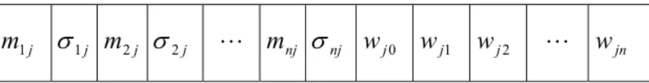
cause partial solutions too similar. Therefore, the algorithm may have less chance to obtain optimal solution. To this end, MGCSE [15], which is a previous evolutionary algorithm and similar to ESP, was proposed for evolving TSK-type neural fuzzy networks. Compare to SANE, MGCSE provide several groups to evaluate each partial solution. Each group in the MGCSE represents a group that consists of the set of the chromosomes that belongs to the partial solution. In MGCSE, the population consists of several sub-populations and each sub-population represents the set of the chromosomes that belongs to one fuzzy rule. The structure of the chromosome is shown in Fig. 2.3. In this figure, each fuzzy rule represents a chromosome that is selected from a group, Psize represents there are Psize groups in a population, and “Mk” represents Mk fuzzy rules are used to construct a TSK-type neural fuzzy network.

Gaussian membership function with mean and deviation, respectively, and w is the weight _ji

with ith dimension and jth rule node.

j

m₁ σ_1j m_2j σ_2j … m_nj σ_nj w_j0 w_j1 w_j2 … w _jn

Figure 2-4: Coding a fuzzy rule of a TNFN into a chromosome in MGCSE.

However, MGCSE have difficulty in scaling to more complex tasks or high input dimension of networks, conduct the problem of the random group selection of fuzzy rules, and the lost of potential fuzzy rules combinations. In consideration of the lost of potential fuzzy rules combinations, Gomez had proposed HESP to accomplish it. Nevertheless, HESP suffers from the problems that the lengths of chromosomes must be the same and the number of neurons has to be assigned in advance. To this end, this dissertation proposes RGLS-HCCA to address the above mentioned problems.

2.4 2D Image Alignment

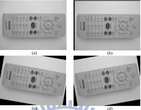
In this subsection, a 2D image alignment task is introduced. Image alignment can be viewed as a mapping between two images by means of a geometric transformation. Typically, geometric transformation contains many types, including affine, similarity, and projective transformation. Among them, affine transformation is the most common used type and it composites of translation, rotation, and scaling. Thus, this paper adopts the affine transformation as the transformation model. Figure 2.5 shows an example of a remote controller with different transformation parameters. In Fig. 2.5 (a), it represents a reference image which other transformed images want to align with. In other words, if the pose of the transformed image is known, then the transformed image can be recovered to the original pose of the reference image by reversing the pose. Thus, a 2D image alignment task defined in this dissertation is to align transformed images with the reference image.

(a) (b)

(c) (d)

Figure 2-5: Example of generating training images with different affine transformation: (a) reference image, (b) translation, (c) clockwise rotation, and (d) counterclockwise rotation.

Since industrial inspection tasks are assumed, area-based alignment methods that adopt global descriptors are recommended. Thus, this study tries to focus on developing a good area-based alignment method. Figure 2.6 illustrates a typical procedure of an area-based 2D image alignment system. As shown in this figure, the sensed image is sent into the descriptor to extract the feature. Then, feed the feature into a pose estimation block to estimate the pose with respect to the reference image. Finally, the estimated affine transformation parameters can be used to align the sensed image with the reference image. Toward this end, seeking accurate affine transformation parameters is the most important fields for aligning images.

Figure 2.7 illustrates an example of aligning 2D images where figure (a) is a reference image, figure (b) is an input image, and figure (c) is a alignment result of using neural network based alignment scheme defined in [44]. In Fig. 2.7 (c), the cross sign denotes the estimated results of Sarnel’s work [44] and from the location of this cross sign, the alignment results is not good enough. The major drawback of such approach is that they have difficulty in applying to align images on a large range of affine transformation. Thus, this dissertation proposes a CNFN-based 2D image alignment method to perform coarse-to-fine alignment of the sensed image and the reference image.

(a) (b)

(c)

Figure 2-7: Example of 2D alignment: (a) reference image, (b) image with an affine transformed, and (c) alignment results of neural network based scheme.

2.5 3D Image Alignment

imaging laser scanner. Each pixel in the range image reflects a range data which indicates a distance from the sensed point to the scanner. In other words, the range data can be considered as a 3D point with respect to the scanner. Thus, the scanner can be a center of a coordinate system to represent each sensed range data. Figure 2.8 presents an example of the range image, intensity image, and a 3D point cloud data. From this figure, the range image utilizes the color bar to represent the range data. The intensity image, which is also generated by the imaging lasers scanner, is used to be the corresponding map of range image. The 3D point cloud data, which is created by transforming range data to Cartesian coordinate, shows the 3D position of each pixel.

Figure 2.9 illustrates the procedure of a 3D image alignment task. From this figure, the 3D scene is scanned by a 3D imaging laser scanner where the size of the scanned scene is 256×256 with 20 degree field of view. The region of interest (ROI) is extracted by using the segmentation algorithm described in [68]. The reference model is a target 3D surface that the ROI wants to align with. Thus, the purpose of the 3D image alignment task is to align the ROI with the reference model.

Figure 2-8: Example of 3D image.

Figure 2-9: Procedure of a 3D surface alignment task Intensity image Range image Coordinate Transformation 3D point cloud 3D scene Segmentation Align ROI Reference Model Alignment Result

According to Chapter 1, a coarse-to-fine technique is a useful way to perform 3D image alignment tasks. In consideration of coarse image alignment, common methods [45] and [46] utilized PCA [51] for coarsely aligning two images due to its high-speed performance. In consideration of traditional fine alignment methods, iterative closest point (ICP) [52] is a typical method to iteratively calculate the rigid-body transformation to minimize the cost function.

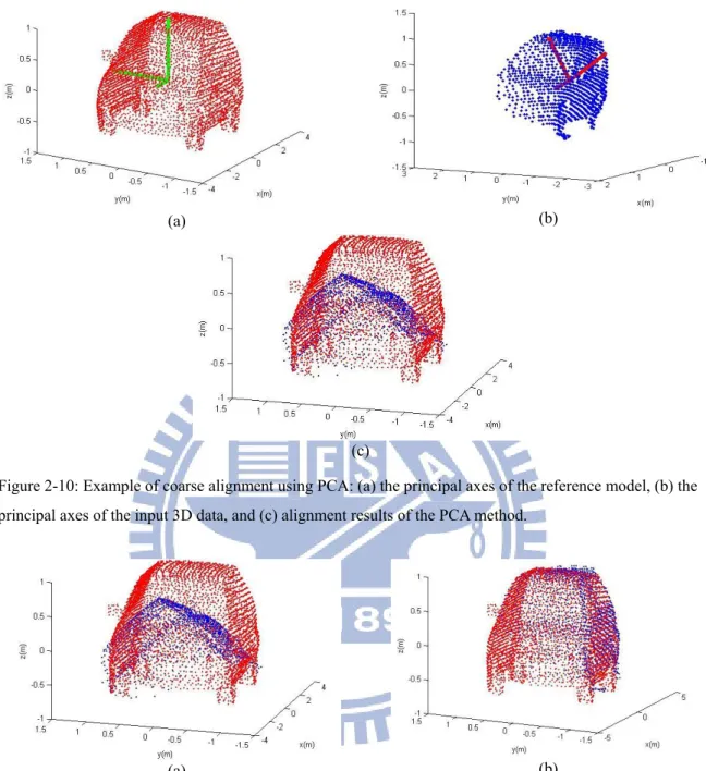
Figure 2.10 illustrates an example of aligning an input 3D point with reference model using PCA. From this figure, (a) and (b) represents the principal axes of a 3D reference model and input 3D point data, respectively. Figure 2.10 (c) depicts the alignment results of PCA method. From Fig. 2.10 (a)-(c), we can know that since the input laser scanned 3D data is partial, its principal axes would be askew with respect to the 3D reference model and such case results in the large alignment error of PCA method (seen from Fig. 2.10 (c)). Based on this fact, this dissertation will propose a TNFN-based coarse alignment method that utilizes the pose estimation to replace of aligning principal axes.

Figure 2.11 illustrates an example of performing ICP fine alignment where figure (a) is the initial alignment yielded by PCA coarsely alignment and figure (b) is final fine alignment performed by ICP. Although ICP can get a good result for fine alignment, its heavy computational cost in searching corresponding points is a problem. To this end, this paper proposed a TNFN-based fine alignment method which combines surface modeling and the downhill simplex optimization method to improve the problem.

Figure 2-10: Example of coarse alignment using PCA: (a) the principal axes of the reference model, (b) the principal axes of the input 3D data, and (c) alignment results of the PCA method.

Figure 2-11: Example of fine alignment using ICP: (a) the initial alignment yielded by PCA and (b) alignment results of the ICP method.

(a) (b)

(c)

Chapter 3

Regularized Least Squares Based Hierarchical

Cooperative Coevolutionary Algorithm

The learning process of RGLS-HCCA is shown in Fig. 3.1. As show in this figure, RGLS-HCCA involves two major evolutions: parameter level evolution (PLE) and structure level evolution (SLE). The blocks of inserting good networks and inserting good neurons (i.e. good fuzzy rules) are the connection between the parameter and structure level evolution. These two operations indicate that good evolved results in one level evolution would be transferred to another level evolution. Once receiving good neurons or networks, the received chromosomes would be mated with other old chromosomes to yield some new offspring. Therefore, by exchanging the good information between two levels of evolution, we have more chance to find the global optimal solution.

This chapter is divided into two subsections to introduce the proposed two-level evolution. In Section 3.1, parameter level evolution is discussed. Section 3.2 describes how structure evolution works.

Figure 3-1: Learning process of RGLS-HCCA.

3.1 Parameter Level Evolution

In this subsection, we will discuss the parameter level evolution (PLE). In PLE, it aims to determine not only the suitable fuzzy rules of TNFN automatically but also the suitable individuals used to construct a TNFN. Regarding the former aim, PLE proposes a self-regulated mechanism (SRM) to determine the number of fuzzy rules automatically. SRM utilizes the probability vector to represent the suitability of TNFN with different fuzzy rules. In Fig. 3.2, SRM codes the probability vector

k

M

P to represent the suitability of a TNFN

with Mk rules where the number of fuzzy rules is limited to a certain bound, i.e., [Mmin, Mmax]. After the SRM is carried out, the probability of the suitable number of fuzzy rules in a TNFN will increase, and the probability of the unsuitable number of fizzy rules in a TNFN will decrease. Therefore, the number of fuzzy rules would be self-regulated. Regarding the later

aim, although SRM can determine the suitable number of rules, there is a need to identify the suitable groups used to select individuals to construct TNFN. More specifically, we should consider the well-performing groups of individuals to cooperate for producing better a generation than the current one. To face this issue, this study proposes a data-mining based selection method (DMSM) to determine which groups should be used to select individuals.

The DMSM involves two major parts, namely, finding frequent patterns and mining association rules. Regarding the former, the FP-growth algorithm [27] is used to find the frequent patterns that do not have candidate generation. Regarding latter, association rules are identified by using the confidence value. In DMSM, the FP-growth is used to find the sets of groups that occur frequently from transactions. In this paper, a “transaction” refers to the collection of groups that have good or bad performance. After the candidate sets of frequently occurring groups are found, DMSM identifies the association rules by setting the suitable confidence and uses the found association rules to determine Mk groups that are used to select

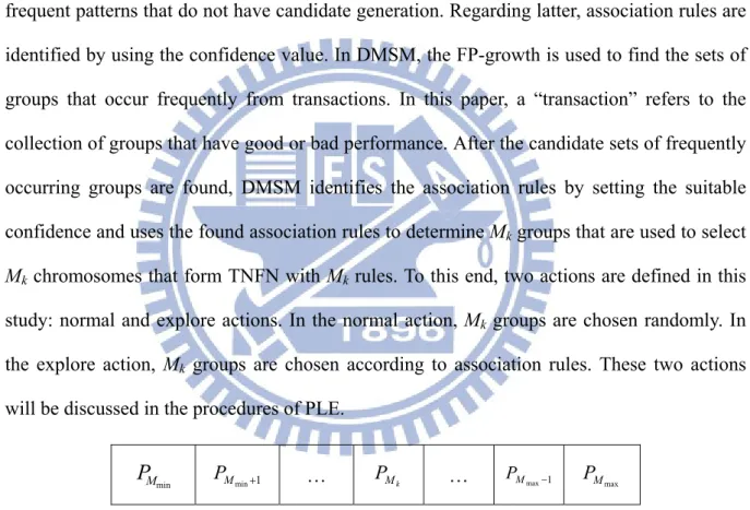
Mk chromosomes that form TNFN with Mk rules. To this end, two actions are defined in this study: normal and explore actions. In the normal action, Mk groups are chosen randomly. In the explore action, Mk groups are chosen according to association rules. These two actions will be discussed in the procedures of PLE.

min

M

P

P_{Mmin+1 …} P _{Mk …} PMmax−1 PMmax

Figure 3-2: Coding the probability vector to represent the suitability of a TNFN with Mk rules.

population, and Mk indicates that there are Mk rules used in TNFN construction. In addition, PLE adopts the variable length of a combination of chromosomes with RGLS method to construct a TNFN. Thus, the length of combined chromosomes to construct TNFNs can be different.

Figure 3-3: Structure of chromosomes to TNFN construction in PLE.

After discussing the structure of chromosomes to construct TNFNs, details of the coding step for PLE and RGLS method are described as follows:

(1) Coding Step:

The coding structure of chromosomes in the proposed PLE is shown in Fig. 3.4. This figure describes an antecedent part of a fuzzy rule that has the form in Eq. (2.5), where m _ij

and σ_ij represent a Gaussian membership function with mean and deviation of ith dimension and jth rule node, respectively. Besides, a pair of (m,σ ) indicates a neuron in Layer 2 of a TNFN. Evolving an antecedent part of a fuzzy rule is likely to evolve a neuron which is a parameter of a neural network. Thus, the evolution of this level is called a parameter (i.e. neuron) level evolution.

Figure 3-4: Coding an antecedent part of a fuzzy rule into a chromosome in PLE. (2) RGLS method:

Assume a TSK-type neural fuzzy model composed of m fuzzy rules as the following form:

R IF x_j : 1 is A1jand…and xn is A , THEN nj yj =woj +w1jx1+L+wnjxn, (3.1)

where j=_{1 L}, ,m and j i

A is the linguistic part with respect the input i and Rule j. From Eq. (3.1), the output can be written as:

ˆ_{1 1} ˆ_{2 2} ˆ , 1 1 m m m j j m j j j y u y u y u u y u y = = + + +

∑

∑

= = L (3.2)

where u_j is the firing strength of Rule j, and uˆ_j =u_j /(u₁+_L+u_m). Then it is possible to express the equation above into the form:

y u w w x w x u w w x wmx_n aW n m m m n n + + + + + = + + + = ˆ ( 1 ) ˆ ( _{0 1 1} ) 1 1 1 1 0 1 L L L , (3.3) where W W W W w wj T j m n j j T T m T _{] , [ ] , 1, ,} [ _{1 L} = _0L = _L = , and )] ˆ ˆ ˆ ( ) ˆ ˆ ˆ ( ) ˆ ˆ ˆ [(u₁u₁x₁ u₁x_n u₂u₂x₁ u₂x_n u_mu_mx₁ u_mx_n a= _{L L L L} .

solution can be written as follows: d T T_{A I A Y} A Wˆ _{=( +λ )}−1 _{, (3.5)}

where λ is a regularization parameter which adjusts the smoothness. Thus, by getting Eq. (3.5), we finish the estimation of the consequent part of fuzzy rules. Based on this fact, this dissertation utilizes RGLS to calculate the consequent part of a TSK-type neural fuzzy network. This operation would not only reduce the number of parameters that must be trained but also increase the convergence rate of the evolutionary algorithm. Thus, the phenomenon of reducing training number and increasing convergence rate would promote the evolutionary algorithm to adapt the neural network to more complex tasks.

The learning process of PLE involves seven operators: initialization, self-regulated mechanism, data-mining based selection method, fitness assignment, reproduction, crossover, mutation, and insert good networks. The whole learning process is introduced below:

a. Initialization: Before we start the parameter level evolution, the initial groups of

individuals should be generated. Thus, initial groups are generated randomly within a predefined range. The following formulations show how to generate the initial chromosomes in each group:

Deviation: Chrg, c[p]=random [σ_min, σ_max],

where p=2, 4,…, 2n; g=1, 2,…, Psize; c=1, 2,…, NC, (3.6)

Mean: Chrg, c[p]= random [m_min, m_max],

where p=1, 3,…, 2n-1, (3.7) where Chrg, c represents cth chromosome in the gth group, NC is the total number of chromosomes in each group, p represents the pth gene in a Chrg, c, and [σmin, σmax], [mmin,

max

m ] represent the predefined range to generate the chromosomes.

b. Self-regulated mechanism (SRM): To select fuzzy rules automatically, PLE proposes

self-regulated mechanism encodes the probability vector k

M

P to stands for the suitability of a TNFN with Mk rules. In addition, in SRM, the minimum and maximum number of rules must be predefined to limit the number of fuzzy rules to a certain bound, i.e., [Mmin, Mmax]. The processing steps of SRM are described as follows:

Step 0. Initialize the probability vectors

k M P : . , , 1 , where , 5 . 0 max min min M M M M P k Mk L + = = (3.8) Accumulator =0. (3.9)

Step 1. Update the probability vectors

k

M

P according to the following procedures: (1) Evaluate the fitness value of TNFN with Mk rules:

1 , then ) _ ( if + = + = − ≥ fitcount fitcount Fitness fit fit essvalue ThreadFitn Fitness Best Fitness k k k k k M M M M M , (3.10)

where Fitness_Mk represents the fitness value of TNFN with Mk rules,

k

M

Fitness

Best_ represents the best fitness value of TNFN with Mk rules, fit_Mk is the sum of the fitness values of the TNFN with Mk rules and fitcount is a count as Eq. (3.10) satisfies.

(2) Calculate the average fitness value: , / fitcount

fit

∑

= = max min _ M M M M M M k k k k Avgfit Avgfit value Upt , (3.13) ⎪⎩ ⎪ ⎨ ⎧ − = ≤ + = otherwise ), * _ ( if ), * _ ( r value Upt P P Avgfit Avg r value Upt P P k k k k k k k M M M M M M M , (3.14) where k M value

Upt _ is a update value for Mk fuzzy rules and PM_k is the

probability vector, and r is a predefined ratio value.

Step 2. Determine the selection times of TNFN with different rules according to the

probability vectors as follows: k

M

Rp =(Selection_Times)*(P_Mk /Total_Velocy), (3.15)

∑

= = max min _ M M M M k k P Velocy Total , (3.16)

where M_k =M_min, M_min+1,_L, M_max, Selection _Times represents the total selection times in each generation and Rp_Mk represents the selection times of TNFN with Mk rules in one generation.

Step 3. In SRM, to prevent suitable selection times from falling into the local optimal solution,

we uses two different procedures to update P . Such actions are defined as follows: _Mk

Procedure 1: update the probability vector

1 then , _ _ if , 2 to 1 Steps do then , if + = = ≤ r Accumulato r Accumulato Fitness Best Fitness Best SRMTimes r Accumulato g (3.17)

where SRMTimes is a predefined value, Best _Fitness_g represents the best fitness value of the best combination of chromosomes in the gth generation, and Best _Fitness represents the best fitness value of the best combination of chromosomes in the current generations.

process for SRM. Since the amount of the computation in Eq. (3.11)-(3.13) is not heavy (depend on the number of Fitness and it is often not much), updating a _Mk P in Eq. (3.14) _Mk

is also less computation. It implies that SRM is not a heavy computation procedure.

Procedure 2: initialize the probability vector

, 0 and 0 Step do then ,

if Accumulator >SRMTimes Accumulator = (3.18) If Eq. (3.18) is satisfied, it indicates that the suitable selection times may fall into the local optimal solution. At this time, the processing step of SRM should return to Step 0 to initialize the probability vectorP . _Mk

c. The data-mining based selection method (DMSM):

After operating SRM, the selection times of TNFNs with different numbers of rules are determined. Thereafter, PLE performs the selection step, which involves the selection of groups and the selection of chromosomes. In selection of groups, this paper proposes DMSM to determine the suitable groups for chromosomes selection to form a TNFN.

In DMSM, suitable groups are selected according to the groups, which conduct from association rules that indicate good performance. To achieve these aims, DMSM utilizes the FP-growth [27] and the association rules mining. Regarding former, the FP-growth is used to identify frequently pattern. It was proposed by Han et al. [27], and it aims to find the frequently occurring patterns that do not have candidate generation. In the proposed DMSM,

that are used to choose chromosomes to form TNFNs with Mk rules. To prevent the selected groups from falling into the local optimal solution, DMSM uses normal and explore actions to select well-performed groups. The details of the DMSM are discussed below:

Step 1. Normal action:

If Accumulator don not exceed the NormalTimes, the current action is the explore action. The aims of this action include two parts: accumulate the transaction set and select groups which are described as follows:

Part 1: Accumulate the transaction set

The transactions are built, as in the following equations:

, ] [ ] [ ) _ ( if g Index e Performanc then i t TNFNRuleSe i n Transactio essvalue ThreadFitn Fitness Best Fitness k k k M j M M = = − ≥ (3.19) , ] [ ] [ ) _ ( if b Index e Performanc then i t TNFNRuleSe i n Transactio essvalue ThreadFitn Fitness Best Fitness k k k M j M M = = − < (3.20)

where i=1 ,2 ,_L ,M_k , M_k =M_min ,M_min +1 ,_L ,M_max , j=1 ,2 ,_L ,TransactionNum , the k

M

Fitness represents the fitness value of TNFN with Mk rules, ThreadFitnessvalue is a predefined value, TransactionNumis the total number of transactions, Transaction_j[i] represents the ith item in the jth transaction, TNFNRuleSet [i]

k

M represents the ith group in

the Mk groups used for chromosomes selection, and PerformanceIndex= g and

b Index e

Performanc = represent the good and bad performance, respectively. Hence, transactions have the form shown in Table 3.1. As shown in Table 3.1, the first transaction means that the three-rule TNFN formed by the first, fourth, and eighth groups have ”good” performance. In contrast, the second transaction indicates that the four-rule TNFN formed by the second, fourth, seventh, and the tenth groups have “bad” performance.

Table 3.1: Transactions in the DMSM. Transaction index Groups Performance Index

1 1,4,8 g

2 2,4,7,10 b

… … …

TransactionNum 1,3,4,6,8,9 g Part 2: Select groups

In the normal action, DMSM selects groups using the following equation:

], , 1 [ ] [ then if Size P Random i GroupIndex s NormalTime r Accumulato = ≤ (3.21) where i=1 ,2 ,_L ,M_k, M_k =M_min ,M_min+1 ,_L ,M_max, Accumulator defined in Eq.(3.21) is used to determine which action should be adopted, GroupIndex represents the selected ith [i] group of the Mk groups, and P indicates that there are _Size P groups in a population in _Size PLE. If the best fitness value does not improve for a sufficient number of generations (NormalTimes), then DMSM selects groups according to explore action.

Step 2. Explore action:

If Accumulator exceeds the NormalTimes, the current action switches to the explore action. The objective of this action is to adopt the notion of DMSM to explore suitable groups in transactions. The major operations of DMSM include FP-growth performing, association rules generating, and suitable groups selecting. The details of these three operations are presented below.

In FP-growth, frequently occurring groups can be found by exploring the FP-tree [27]. After exploring the frequently occurring groups in the FP-tree, FP-growth data mining is completed by the concatenation of the suffix group [27] with the generated frequently occurring groups. Thus, in this paper, frequent groups denote the frequently occurring groups found by FP-growth algorithm.

ii. Association rules generating

Once the frequently occurring groups are found, we can produce association rules from these frequent ones. For the purpose of identifying the association rules with good performance, the frequent groups must combine the groups owing bad performance shown in Table 3.1 to count the confidence degree. The confidence degree can be computed by the following formula: , ) ( ) ( ) ( ) | ( ( ) bad groups frequent supp good groups frequent supp good groups frequent suppgroups frequent good

P frequentgroups good confidence ∪ + ∪ ∪ = = ⇒ (3.22)

where P(good| frequentgroups) is the conditional probability, frequentgroups∪good

or bad means the union of frequent groups and good or bad performance, and

supp( frequentgroups∪goodor bad) stands for the counts of frequent groups with good or bad performance occurring in transactions. Then the rule is valid if

confidence(frequentgroups⇒ good)≥minconf, (3.23) where minconf represents the minimal confidence given by user or expert. Hence, we can infer that if a rule satisfies Eq. (3.23), then the frequent groups can be viewed as the suitable groups, otherwise they would be unsuitable groups. For instance, if the confidence of {1,3,6}=>{g} is bigger than the minimum confidence, then we construct this association rule. This rule indicates that the combination of the first, third, and sixth groups results in “good” performance. After doing so, the frequent groups are conduct to the association rules and generate the AssociatedGoodPool which contains all frequent groups satisfied Eq. (3.23).

iii. Suitable groups selecting

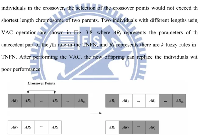
After the association rules are identified, DMSM selects groups according to the association rules. The group indexes are selected from the associated good groups as the following equations: ], [ ] [ ] [ ] , 1 [ where , ] [ then if GoodPool Associated Random q t GoodItemSe q t GoodItemSe w and P Randm w w i GroupIndex es ExploreTim r Accumulato s NormalTime size = ∈ = = ≤ < (3.24)

where ,q=1 ,2 ,_L ,AssociatedGoodPoolNum i=1 ,2 ,_L ,M_k , M_k =M_min ,M_min+1 ,_L ,M_max ,

es

ExploreTim is a predefined value that judge to perform the exploring action, GoodPool

Associated represents the sets of good item set that obtain from association rules,

m GoodPoolNu

Associated presents the total number of sets in AssociatedGoodPool and

] [i

t

GoodItemSe presents a good item set that select from AssociatedGoodPool randomly. In the Eq. (3.24), if M greater than the size of _k GoodItemSet, remain groups are selected by Eq. (3.21).

Step 3. If the best fitness value does not improve for a sufficient number of generations

(ExploreTimes), DMSM selects groups based on the normal action (Step 1).

Step 4. After the Mk groups are selected, Mk chromosomes are selected from Mk groups as follows: , ] [i q Index Chromosome = (3.25)