支援無線區域網路服務品質之改良型公平排程策略

全文

(1)國立交通大學資訊科學系碩士論文. 支援無線區域網路服務品質之改良型公平排程策略. An Enhanced Fair Scheduling for QoS in IEEE 802.11e Wireless LANs. 研究生：曾昆南指導教授：王國禎. 博士. 中華民國九十三年六月.

(2)

(3) 支援無線區域網路服務品質之改良型公平排程策略. An Enhanced Fair Scheduling for QoS in IEEE 802.11e Wireless LANs 研究生：曾昆南. Student：Kun-Nan Tseng. 指導教授：王國禎. Advisor：Kuochen Wang. 國立交通大學資訊科學系碩士論文 A Thesis Submitted to Department of Computer and Information Science College of Electrical Engineering and Computer Science National Chiao Tung University in Partial Fulfillment of the Requirements for the Degree of Master in Computer and Information Science June 2004 Hsinchu, Taiwan, Republic of China. 中華民國九十三年六月.

(4)

(5) 支援無線區域網路服務品質之改良型公平排程策略學生：曾昆南. 指導教授：王國禎博士. 國立交通大學資訊科學系. 摘要隨著無線區域網路越來越受歡迎，對於支援多媒體和確保服務品質的應用程式需求變得比以前更重要。雖然有很多改進原本IEEE 802.11 MAC的機制被提出來，以支援服務品質，但是他們對於高優先權和低優先權的流量會有頻寬分配不公平的現象。我們提出一個分散式加強型公平排程策略來解決上述問題。基於在後退計數器遞減狀態的快速後退機制和依網路負載情況來動態修改後退區間的機制，我們可以強化加強型公平排程策略的效能。我們經由模擬來評估本加強型公平排程策略的效能。實驗結果顯示我們所提出的加強型公平排程策略比分散式公平排程策略高出13%的效能和比分散式公平排程策略低 6%的平均MAC延遲時間，而且兩者有幾乎相等的公平指標。雖然IEEE i.

(6) 802.11e的進階分散式頻道存取機制比加強型公平排程策略和分散式公平排程策略有較好的效能，但是它非常不公平。進階分散式頻道存取機制的免競爭機制是導致高效能、低平均MAC延遲時間和低公平性的主因。我們的加強型公平排程策略非常適合於對頻寬公平分配要求很高的應用程式，如付費應用服務。. 關鍵詞：公平排程策略、IEEE 802.11e、服務品質、無線區域網路。. ii.

(7) An Enhanced Fair Scheduling for QoS in IEEE 802.11e Wireless LANs Student：Kun-Nan Tseng. Advisor：Dr. Kuochen Wang. Department of Computer and Information Science National Chiao Tung University. Abstract As wireless LANs are gaining popularity, the demand for supporting multimedia and QoS-sensitive applications becomes more important than before. Although enhancements to the legacy IEEE 802.11 MAC to support QoS mechanisms have been proposed, they suffer from unfair allocation of bandwidth between high and low priority traffic. We propose a distributed enhanced fair scheduling (EFS) scheme that can conquer the above problem. With a fast backoff mechanism in the backoff timer decrement state and by dynamically adjusting backoff intervals according to the network load, we can enhance the performance of EFS. We evaluate the performance of EFS through simulation. Experimental results show that the proposed EFS has better throughput performance than DFS by 13%, lower average MAC delay than DFS by 6% and the two have nearly equal fairness. Although the enhanced distributed channel access (EDCA) in IEEE 802.11e has better throughput. and delay. performance than EFS and DFS, it has very poor fairness. The contention free burst (CFB) mechanism in EDCA is the main factor that results in good throughput performance, lower average MAC delay and poor fairness. Our EFS is very suitable for applications that needs strict fair bandwidth allocation, such as pay services.. iii.

(8) Keywords：fair scheduling, IEEE 802.11e, quality of service, wireless LAN.. iv.

(9) Acknowledgements Many people have helped me with this thesis. I deeply appreciate my thesis advisor, Dr. Kuochen Wang, for his intensive advice and instruction. I would like to thank all the classmates in Mobile Computing and Broadband Networking Laboratory for their invaluable assistance and suggestions. The support by the National Science Council under Grant NSC92-2213-E-009-078 is also grateful acknowledged. Finally, I thank my Father and Mother for their endless love and support.. v.

(10) Contents Abstract (in Chinese). i. Abstract (in English). iii. Acknowledgements. v. Contents. vi. List of Figures. viii. List of Tables. ix. Chapter 1 Introduction................................................................................................1 Chapter 2 Previous Work............................................................................................4 2.1 The Enhanced Distributed Channel Access (EDCA).......................................4 2.2 The Fast Collision Resolution (FCR) Algorithm .............................................5 2.3 The Distributed Fair Scheduling (DFS) ...........................................................7 2.4 The Distributed Deficit Round-Robin Scheme..............................................11 Chapter 3 Design Approach: Enhanced Fair Scheduling ......................................13 3.1 The EFS Design Framework..........................................................................13 3.2 Dynamically Updating Division_Factor ........................................................21 vi.

(11) Chapter 4 Simulation Model and Simulation Results ............................................24 4.1 Simulation Model...........................................................................................24 4.2 Simulation Results .........................................................................................26 4.2.1 Aggregate Throughput........................................................................26 4.2.2 Fairness Index and Throughput Variance...........................................27 4.2.3 MAC Delay.........................................................................................31 Chapter 5 Conclusions and Future Work................................................................32 5.1 Concluding Remarks......................................................................................32 5.2 Future Work ...................................................................................................32 Bibliography ...............................................................................................................34. vii.

(12) List of Figures. Fig. 1. IEEE 802.11e EDCA IFS relationship............................................................5 Fig. 2. Basic operation of CSMA/CA [10]. ...............................................................7 Fig. 3. The SCFQ algorithm.....................................................................................10 Fig. 4. The DFS maps the output link in SCFQ to the shared medium and the input flows to the traffic from wireless nodes; DFS is a distributed version of SCFQ. ..........................................................................................................................10 Fig. 5. The DDRR mechanism.................................................................................12 Fig. 6. The state transition of EFS. ..........................................................................14 Fig. 7. The backoff timer decrement state................................................................16 Fig. 8. The aggregate throughput of high and low priority flows............................27 Fig. 9. The fairness index of different schemes. ......................................................28 Fig. 10. The throughput obtained by each high priority station (flow)....................30 Fig. 11. The throughput obtained by each low priority station (flow).....................30 Fig. 12. The average MAC delay of different schemes ...........................................31. viii.

(13) List of Tables Table 1：Simulation parameters..............................................................................25 Table 2：Comparison between various schemes.....................................................29. ix.

(14) Chapter 1 Introduction The IEEE 802.11 Wireless LAN is gaining a lot of popularity in recent years because of cost-effectiveness in building a wireless broadband network environment. Mobile computing devices such as portable computers and personal digital assistants become indispensable in our daily activities. With the increasing use of wireless local LANs, there is high demand for supporting multimedia and QoS-sensitive applications. Because the IEEE 802.11 legacy MAC is only suitable for QoS-insensitive applications, the enhancements to the legacy MAC to support QoS mechanisms [14, 15, 16, 17] have been proposed. The enhancements provide service differentiation by statically assigning priorities to classes. A high priority class is assigned a shorter interframe space (IFS) and a shorter contention window (CW) than a low priority class. However, these approaches suffer from unfair allocation of bandwidth between high and low priority traffic. Fair scheduling [1, 7, 19] was designed to overcome the above problem by partitioning the bandwidth fairly between different traffic classes. In the thesis, we propose an enhanced fair scheduling (EFS) scheme based on the distributed fair scheduling (DFS) [2]. The proposed EFS integrates the DFS’s idea of calculating backoff interval of packets and the Fast Collision Resolution’s idea [10] of decreasing backoff timer exponentially. The proposed EFS can provide better throughput and delay performance than DFS and maintain nearly equal fairness.. 1.

(15) Much researches on fair scheduling algorithms for achieving a fair allocation of bandwidth on a shared wired link [1, 7, 18, 19] have been proposed. All fair scheduling algorithms are based on the fluid fair scheduling model [18]. In the model, packet flows are modeled as fluid flows. Fluid fair scheduling guarantees that for an arbitrary time interval [t1, t2], any two backlogged flows i and j are served in proportion to their weights, which are represented by the following equation:. Wi (t1 , t 2 ). φi. =. W j (t1 , t 2 ). φj. (1). where Wi(t1,t2) and ψi are the service amount received (bits) by flow i during time interval [t1, t2] and the weight of flow i, respectively. However, in the real network world, systems handle flows at the granularity of packets rather than bits. Therefore, the main objective of packet fair queuing (PFQ) algorithm is to approximate the Generalized Processor Sharing (GPS) [18] as closely as possible. The GPS is an ideal fluid fair scheduling model. The most famous PFQ algorithm is the weighted fair queuing (WFQ) [22], equivalently a packetized generalized processor sharing (PGPS). However, WFQ has its drawbacks that it is not easy to implement because the cost of maintaining a priority sorting queue and the overhead of computing the virtual system time is very high. Self clocked fair queuing [7] and start time fair queuing [19] reduced implementation complexity of WFQ. The PFQ algorithms developed for wired networks cannot be directly applied to wireless networks because of bursty and location-dependent errors in wireless channels. In the. 2.

(16) next chapter, we will describe classical fair scheduling algorithms that emulated the PFQ algorithm in wireless networks. The subsequent chapters of this thesis are organized as follows. In Chapter 2, we describe previous work in this research area. We describe the proposed EFS in detail In Chapter 3. In Chapter 4, we evaluate the throughput and delay performance, and the fairness index of the proposed EFS via simulation. In Chapter 5, we summarize our current work and address future prospect.. 3.

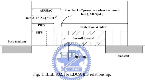
(17) Chapter 2 Previous Work We will review the enhanced distributed channel access (EDCA) [6, 13], the fast collision resolution (FCR) [10], distributed fair scheduling (DFS) [2], and distributed deficit round-robin (DDRR) [8] schemes in this chapter. The FCR contributed to throughput performance improvement. The DFS incorporated fair queuing to wireless LANs. The DDRR translated user requirements into appropriate IFSs to provide service differentiation.. 2.1 The Enhanced Distributed Channel Access (EDCA) The fundamental MAC protocol [3] used in 802.11 can not support QoS-sensitive applications. Therefore, the 802.11e draft introducing the enhanced distributed channel access (EDCA) and hybrid coordination function (HCF) to support QoS are currently under discussion [6]. Service differentiation is achieved through the introduction of access categories (ACs). Each AC on a station contends for a transmission opportunity (TXOP) [6] and has its own transmission queue. Each transmission queue has a different interframe space (called arbitrary interframe space – AIFS[AC]), and a different set of contention window limits (CWmin[AC] and CWmax[AC]). Fig. 1 illustrates the detailed IFS relationship. Each AC start its backoff procedure when the medium is idle for AIFS[AC] time. When an AC start its. 4.

(18) backoff procedure, it chooses a backoff interval uniformly distributed in [0, CWmin[AC]]. The AC will transmit its packet immediately when the backoff interval counts down to zero. Although the 802.11e support better QoS than the legacy 802.11, it suffers from unfair allocation of bandwidth between high and low priority traffic and has high throughput variability. Randomness in accessing the medium is the main factor resulting in high throughput variability.. AIFS[AC]. Start backoff procedure when medium is free ≥ AIFS[AC]. min AIFS[AC] = DIFS PIFS. Contention Window. SIFS busy medium. Backoff interval. Slot time. transmit. Fig. 1. IEEE 802.11e EDCA IFS relationship.. 2.2 The Fast Collision Resolution (FCR) Algorithm The main deficiency of the IEEE 802.11 MAC protocol [3] comes from packet collisions and wasted idle slots due to backoffs in each contention cycle (as shown in Fig. 2). For example, when the number of active nodes is very large, there are too many nodes backed off with small contention windows, hence many retransmission attempts will most likely collide again in the future. An active node can be in two modes at each contention cycle, namely, the transmitting mode when it wins a contention and the deferring mode when it loses a contention. When a node transmits a packet, the result is either successful or unsuccessful collision. Therefore, a node 5.

(19) will be in one of the following three states at each contention cycle: a successful packet transmission state, a collision state, and a deferring state.. The fast collision. resolution (FCR) [10] algorithm aimed to resolve the collisions quickly by increasing the contention windows sizes of both the colliding nodes and the deferring nodes in the contention resolution. The FCR regenerates the backoff timers for all potential transmitting nodes to avoid possible future collisions. The FCR algorithm preserves the simplicity for implementation, just like the IEEE 802.11 MAC. The FCR algorithm has following characteristics [10]: 1). Use a much smaller initial (minimum) contention window size CWmin than that in the IEEE 802.11 MAC [10];. 2). Use a much larger maximum contention window size CWmax than that in the IEEE 802.11 MAC [10];. 3). Increase the contention window size of a station when it is in either collision state and deferring state [10];. 4). Reduce the backoff timers exponentially when a prefixed number of consecutive idle slots are detected [10].. Items 1) and 4) attempt to reduce the average number of idle backoff slots for each contention cycle [10]. Items 2) and 3) are used to quickly increase the backoff timers, hence quickly decrease the probability of collisions [10]. Item 3) is the major difference from that of the IEEE 802.11 MAC. In the IEEE 802.11 MAC, the contention window of a station is increased only when it experiences a transmission failure. In the FCR algorithm, the contention window of a station will increase not only when it experiences a collision but also when it is in the deferring mode and. 6.

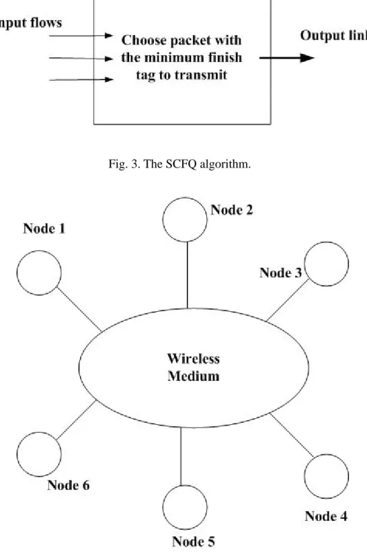
(20) senses the start of a new busy period.. Fig. 2. Basic operation of CSMA/CA [10].. 2.3 The Distributed Fair Scheduling (DFS) Some schemes using fair scheduling were designed to overcome the unfair problem. This kind of schemes can provide relative differentiation, for example specifying that one type of traffic should get twice as much bandwidth as some other type of traffic. For instance, Vaidya et al. [2] proposed Distributed Fair Scheduling (DFS), attempting to emulate Self-Clocked Fair Queuing (SCFQ) [7]. SCFQ is a centralized algorithm for packet scheduling on a link shared by multiple flows as shown in Fig. 3. The central coordinator maintains a virtual clock and at any given time t, v(t) represents the virtual time. Let Pik denote the kth packet arriving on flow i. Let Aik is the real time of arrival for packet Pik. Let Lik denote the size of the packet Pik. A start tag Sik and a finish tag Fik are associated with each packet Pik. The algorithm is as follows [2]:. 7.

(21) 1.. Fi 0 = 0, ∀i .. 2.. On arrival of packet Pi k , the packet is stamped with start tag S ik using following equation: S ik = max{v ( Aik ), Fi k −1}. 3.. A finish tag Fi k for each packet Pi k is calculated as: Fi k = Sik +. Lki. φi. where φi is the weight of flow i . 4.. Initially the virtual clock v(0) is set to 0. The virtual time is updated after a new packet is transmitted. When a packet begins transmission on the output link, the virtual clock is set equal to the finish tag of that packet .. 5.. Packets are selected for transmission in an ascending order of finish tags.. In the SCFQ algorithm, the start and finish tags are calculated when a packet arrives in a flow. Alternatively, the start tag can be calculated when a packet reaches the front of its flow. If the packet arrives when the flow is empty, the time fik is the real time when the packet reaches the front of its flow. If the flow is not empty, fik is the real time when packet Pik-1 finishes the transmission. Thus the start tag for a packet can be calculated as. S ik = v ( f i k ). (2). Like SCFQ, DFS determines the packet transmission based on the finish tag of 8.

(22) each packet and the virtual time is updated in the same way as that in SCFQ. DFS attempts to map the shared wireless medium to the output link and the input flows paradigm of SCFQ. As shown in Fig. 4, the output link in Fig. 3 is mapped to the shared wireless medium and the input flows are mapped to the flows from each node. In the DFS, a packet with the smallest ratio between its length and weight receives the highest priority to transmit. The main idea of this scheme is to pick a backoff interval proportional to the finish tag of the packet. It attempted to emulate the Self-Clocked Fair Queuing (SCFQ) [7] in a distributed manner so as to transmit the packet with the minimum finish tag first. A backlogged node i picks a backoff interval Bi as a function of its weight, ϕi , and packet length Li, as follows: Bi = ⎣⎣Scaling _ Factor * Li / ϕ i ⎦ * ρ ⎦ .. (3). Where ρ , a random variable uniformly distributed in [0.9, 1.1], which is introduced to reduce the possibility of collisions [2]. Since flows with high weights get shorter backoff interval than flows with low weights, differentiation will be achieved. Furthermore, the procedure of calculating backoff interval takes the size of packets into account. This will cause small packets to get shorter backoff intervals than large packets, allowing a station with small packets to send more often so that the same amount of data is sent [2]. When a collision occurs, a new backoff interval is calculated using the backoff procedure of the IEEE 802.11 standard [3] where the initial contention window is assigned 4 [2]. The reason for choosing such a short contention window although a collision has occurred is that DFS tried to maintain fairness among nodes, and thus colliding stations should be able to send packets as soon as possible. However, mapping the QoS requirement to the weight is complicated.. 9.

(23) Fig. 3. The SCFQ algorithm.. Fig. 4. The DFS maps the output link in SCFQ to the shared medium and the input flows to the traffic from wireless nodes; DFS is a distributed version of SCFQ.. 10.

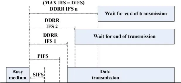
(24) 2.4 The Distributed Deficit Round-Robin Scheme The distributed deficit round-robin (DDRR [8]) QoS scheme is based on the concept of DRR scheduling [1] at the MAC layer of IEEE 802.11. As shown in Fig. 5, the mechanism translates user requirements into appropriate interframe spaces to provide service differentiation and achieves fairness by making use of deficit round-robin fair scheduling [1]. Traffic at each mobile station is categorized into classes with different QoS requirements. A traffic class requiring high throughput receives a fast service quantum rate [8]. Each traffic class maintains a deficit counter of accumulated quanta and can transmit only when its deficit counter achieves a minimum requirement. If the deficit counter of a traffic class falls below a minimum requirement, the traffic class must wait until its deficit counter becomes higher than the minimum requirement. The deficit counter is reduced by the length of the transmitted frame. The deficit counter value is translated into an appropriate interframe space. A traffic class with a smaller interframe space will access the medium first than that with a higher interframe space. A mobile station will transmit its frame immediately after the medium has been free for the interframe space period. If the medium is busy, the mobile station waits for it to become idle, and then immediately transmits after the medium has been free for the new interframe space period. In the DDRR scheme, it eliminates the backoff algorithm because of its contribution to large variation in throughput and delay [14]. Instead, the interframe space value resulting from a deficit counter is multiplied by a random number between 1 and a value β > 1 to reduce collision probability [14]. The DDRR suffers from high collision probability when the number of mobile stations is large.. 11.

(25) Fig. 5. The DDRR mechanism.. 12.

(26) Chapter 3 Design Approach: Enhanced Fair Scheduling We first describe our EFS design framework, including the state transition and the mechanism in each state. Then, we describe how we dynamically update the Division_Factor.. 3.1 The EFS Design Framework We propose an efficient fair scheduling scheme by integrating some of ideas from the DFS scheme [2] and the FCR [10]. The proposed EFS borrows the DFS’s idea of calculating backoff interval of packets and the FCR’s idea of decreasing backoff timer exponentially. The goal of the proposed EFS is to provide fair bandwidth allocation and good throughput by reducing idle backoff slot time. The essential idea of the proposed EFS is to choose a backoff interval that is proportional to the finish tag of a packet to be transmitted and decrement the backoff timer exponentially when consecutive idle slots are detected. We now describe the design approach in detail. We assume that all packets at a node belong to a single flow as proposed in [2]. In a multiple flows case, when station i needs to select the next packet that it will attempt to transmit, it selects the packet with the smallest finish tag among packets at the front of all backlogged flows at station i. When packet Pik reaches the front of its queue, it is tagged with a start tag and a finish tag. Pik represents the kth packet arriving at the flow at station i. Sik, the start tag of Pik, is 13.

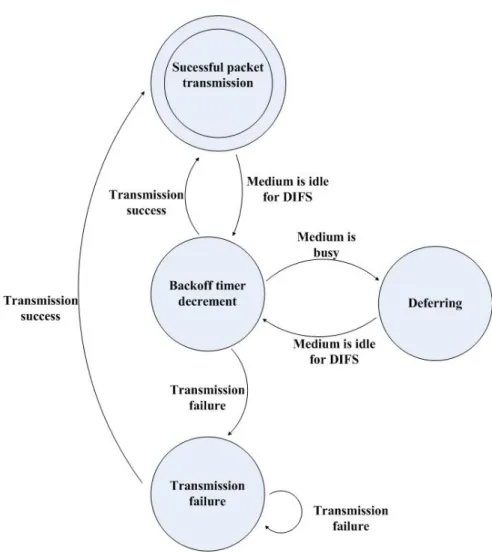
(27) calculated as Sik=v(aik), where aik represents the real time when packet Pik reaches the front of the flow. Finish tag Fik is assigned as follows:. Fi k = S ik + Scaling _ Factor ×. Lki. φi. (4). where Lik represents the length of packet Pik and φi represents the weight of station i . An appropriate choice of the Scaling_Factor allows us to choose a suitable scale for the virtual time.. Fig. 6. The state transition of EFS. 14.

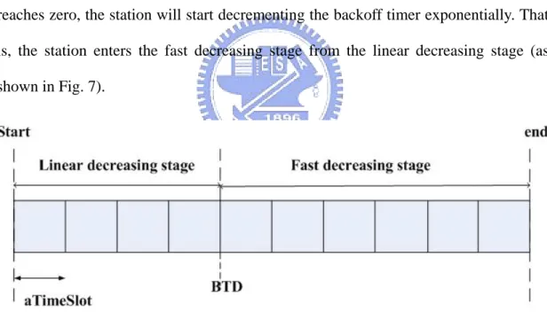
(28) The next step is to choose a backoff interval such that a packet with smaller finish tag will be assigned a smaller backoff interval. This step will be performs in the successful packet transmission state. An active station can be in two modes at each contention cycle, namely, the transmitting mode when it wins a contention and the deferring mode when it loses a contention. When a station transmits a packet, the result is either successful or failed. Therefore, a station will be in one of the following four states at each contention cycle: a successful packet transmission state, a backoff timer decrement state, a transmission failure state, and a deferring state. Fig. 6 shows the state transition of the EFS. The operation of the proposed EFS is described as follows according to the state of a station is in: 1) Backoff timer decrement state: If an active station senses the medium idle for a slot, then it will start decrementing its backoff timer by aSlotTime, as shown in equation (5):. Bnew = Bold − aSlotTime .. (5). where Bold means the old backoff interval and Bnew means the new backoff interval. When the backoff timer reaches to zero, the station will transmit a packet immediately. If there are BTD (Backoff Threshold) consecutive idle slots being detected, its backoff timer will be decreased much faster according to equation (6):. 15.

(29) Bnew = Bold / DF. (if Bnew ＜ aSlotTime, then Bnew = 0 ).. (6). where DF represents Division_Factor. BTD is a constant parameter which will be clear later and the DF parameter will be modified dynamically according to the network load condition. The value of DF can determine the speed of decreasing the backoff interval. The algorithm of modifying DF will be explained in detail later. A station can maintain a counter (called BTD Counter) whose default value is equal to BTD. When the station detects an idle slot time, it decrements its BTD counter by one. When the BTD counter reaches zero, the station will start decrementing the backoff timer exponentially. That is, the station enters the fast decreasing stage from the linear decreasing stage (as shown in Fig. 7).. Fig. 7. The backoff timer decrement state. For example, consider two flows, flow 1 at station 1 with weight 0.1 and flow 2 at station 2 with weight 0.05. Let the packet size be 1000 bytes, the Division_Factor (DF) be 1.5, the Backoff Threshold (BTD) be 60, and the Scaling_Factor be 0.02. The value of Scaling_Factor × PacketSize/weight is the backoff interval (The detail of. 16.

(30) choosing a backoff interval will be illustrated in “3) successful packet transmission state” and for simplicity, we assume that ρ is 1). Thus, the backoff interval will be 200 time slots for flow 1, and 400 time slots for flow 2. When an idle slot is detected, the backoff interval will be 199 time slots for flow 1, and 399 time slots for flow 2, respectively. Each flow will subtract one slot time from its backoff interval until there are 60 consecutive idle time slots being detected. Suppose that there are 60 consecutive idle slots being detected. Now the backoff interval is 140 time slots for flow 1 and 340 time slots for flow 2. Then when an idle slot is detected, the backoff interval will be 93 (140/1.5) time slots for flow 1 and 226 (340/1.5) time slots for flow 2. When an idle slot is detected again, the backoff interval will be 62 (93/1.5) time slots for flow 1 and 150 (226/1.5) time slots for flow 2. The rest may be deduced by analogy. The backoff interval of flow 1 will reach zero first, and then flow 1 will transmit its packet immediately. 2) Transmission failure (packet collision) state: Each station must maintain a CollisionCounter that counts the number of successive collisions. If a station notifies that its packet transmission has failed possibly due to a packet collision, then the station must react with the following procedure: (i) It increments CollisionCounter by 1 (ii) It chooses a new Backoff interval uniformly distributed in. 1 CollisionCounter −1 ⎢ ⎥ × K ⎥] [1, ⎢(1 + ) DF ⎣ ⎦. where K is a constant parameter. The station will choose a small backoff interval in the range [1, K ] after the first collision for a packet. The station will choose a backoff interval in the range. 17.

(31) [1, ⎣(1 + 1 / DF ) × K ⎦] if collision occurs again. To protect against the situation when too many stations collide, the range for the backoff interval grows exponentially with the number of consecutive collisions. The station with higher DF than others will access the medium with a higher probability. The motivation for choosing a small backoff interval after the first collision is that since the colliding station was a potential winner of the contention for channel access, it is the colliding station turn to transmit in the near future. Therefore, the backoff interval is chosen to be small to increase the probability that the colliding station wins the contention soon. We set K to 8 while in the DFS K is set to 4. The reason for setting K to 8 is that since the proposed EFS includes a fast decreasing stage of the backoff interval, we double its value to reduce the collision probability. For example, assume that flow 1 with DF 1.4 at station 1 and flow 2 with DF 1.0 at station 2 collide and that K is equal to 8. Then flow 1 and flow 2 will increment their CollisionCounter’s by 1 and pick a new backoff interval uniformly distributed in [1, 8]. Suppose that the DF of flow 1 and the DF of flow 2 remain the same and flow 1 and flow 2 will collide again after picking their new backoff intervals. Then flow 1 and flow 2 will increment their CollisionCounter’s by 1, flow 1 will pick a new backoff interval uniformly distributed in [1, 13] ( ⎣(1 + 1/1.4) × 8⎦ = 13 ), and flow 2 will pick a new backoff interval uniformly distributed in [1, 16] ( ⎣(1 + 1 / 1) × 8⎦ = 16 ). Suppose that unfortunately flow 1 and flow 2 collide again after picking their new backoff intervals. Flow 1 and flow 2 both increment their CollisionCounter’s by 1 again and now their CollisionCounter’s are equal to 2. Thus, flow 1 will pick a new backoff interval uniformly distributed in [1, 23] ( ⎣(1 + 1 / 1.4) 2 × 8⎦ = 23 ) and flow 2 will pick a new backoff interval uniformly distributed in [1, 32] ( ⎣(1 + 1 / 1) 2 × 8⎦ = 32 ). Thus, we let a high DF flow get a higher probability to access the medium than a low DF. 18.

(32) flow. 3) Successful packet transmission (choosing a backoff interval) state: If a station i successfully transmits a packet with finish tag Z at time t, it will pick a suitable backoff interval Bi for its next packet as proposed in [2] and it sets its virtual clock vi equal to max(vi(t), Z). The backoff interval is derived from equation (4). Suppose the station i will transmit its next packet, Pik.. The station i will tag the packet with a. finish tag. This step is performed at time aik. Thus, station i picks a backoff interval Bi for packet Pik, as a function of Fik and the current virtual time vi(aik), as follows:. Bi = ⎣Fi k − v(aik )⎦. (7). We combine equation (4) with equation (7) and observe that, since S ik. = v ( a ik ) ,. equation (7) reduces to:. ⎢ Lk B i = ⎢ ( Scaling _ Factor × i φi ⎣. ⎥ )⎥ ⎦. (8). Finally, we will randomize the Bi as shown in equation (9). The meaning of Lik and ψi have been described before. ρ is a random variable uniformly distributed in the range [0.9, 1.1] to reduce the possibility of collisions. After deciding the value of Bi, we assign Bold the value of Bi to preserve Bi which will be used in the deferring state. Bold is used in the backoff timer decrement state.. 19.

(33) ⎢ Lk Bi = ⎢ ρ × ( Scaling _ Factor × i φi ⎣. ⎥ )⎥ ⎦. (9). In this state, the station must reset its CollisionCounter to zero and the BTD Counter to BTD. 4) Deferring state: Each transmitted packet is tagged with a finish tag. So when at time t station i hears a packet with finish tag Z, it calculates the difference between Z and the current virtual clock vi(t)., i.e. ∆ = ( Z − vi (t )) . If station i is in the fast decreasing stage with ∆ > 0 , it resets its Bi according to equation (10).. max{ Bold ,( Bi − ∆ )}. (10). and then resets Bold to Bi. The reason we preserve the value of Bi is clear here. In order to maintain fairness, this procedure is necessary since we incorporate a fast backoff mechanism. Finally, the station i sets its virtual clock vi equal to max( v i ( t ), Z ) . For example, consider two flows, flow 1 at station 1, and flow 2 at station 2, with weights 0.2 and 0.1, respectively. Let the packet size be 1000 bytes, the. Division_Factor (DF) be 1.5, the Backoff Threshold (BTD) be 60, and the Scaling_Factor be 0.02. Then, the backoff interval will be 100 time slots for flow 1, and 200 time slots for flow 2. For simplicity, we also assume that ρ used for calculating a backoff interval is 1.0 in this example. Then, flow 1 will choose a backoff interval of 100 time slots for all its packets and flow 2 will choose a backoff 20.

(34) interval of 200 time slots for all its packets. As a result, on average, the number of packets transmitted by flow 1 is 2 times than the number of packets transmitted by flow 2. However, since we introduce the fast backoff mechanism, we must recalculating a backoff interval to maintain fairness. When an idle slot is detected, the backoff interval will be 99 time slots for flow 1, and 199 time slots for flow 2, respectively. Each flow will subtract one slot time from its backoff interval until there are 60 consecutive idle time slots being detected. Suppose that there are 60 consecutive idle time slots being detected. Now the backoff interval is 40 time slots for flow 1 and 140 time slots for flow 2. Then when an idle slot is detected, the backoff interval will be 26 (40/1.5) time slots for flow 1 and 93 (140/1.5) time slots for flow 2. When an idle slot is detected again, the backoff interval will be 17 (26/1.5) time slots for flow 1 and 62 (93/1.5) time slots for flow 2. The rest may be deduced similarly. The backoff interval of flow 1 will reach zero first, and transmit its packet immediately. After flow 1 transmits its packet, the backoff interval of flow 2 is 5. If we did not incorporate the fast backoff mechanism, the backoff interval of flow 2 should be 100. Thus we must recalculate the backoff interval of flow 2. The new backoff interval of flow 2 is 100 (max {5, 200－100}). One notable point is why we select max in equation (10). The consideration is that when a station i receiving a packet just enters the fast decreasing stage, the Bold of the station may be greater than. Bi－△. At this moment, resetting the backoff interval, Bi, to Bold is more appropriate.. 3.2 Dynamically Updating Division_Factor In order to take into account the network load condition for Division_Factor adaptation, we use a measurement scheme similar to [11] to get the related network information. We use the number of collisions as an indicator of the network load condition. The time domain is divided into continuous measurement periods (MPs) 21.

(35) with specified period size. A measurement period (MP) is defined as the number of time slots. When the kth measurement period, denoted by MPk, expires, the station summarizes the network load condition indicator δ (k ) [11] during MPk as follows:. δ (k ) =. nc ns. (11). where nc is the number of collisions which occurred during MPk, and ns is the total number of packets sent during MPk. Because δ (k ) cannot precisely represent the long-term network load condition, we also use an estimator of Exponentially Weighted. Moving Average [11] to smoothen the estimated value of each measurement period. The average network load condition indicator during MPk, denoted by δ avg (k ) is computed as follows:. δ avg ( k ) = θ × δ avg ( k − 1) + (1 − θ ) × δ ( k ). (12). where 0 < θ < 1 . We set θ to be 0.8, as proposed in AEDCF [11]. The. Division_Factor (DF) will be modified every MP according to the following condition:. ∆ k = δ avg (k ) − δ avg (k − 1). 22. (13).

(36) If ∆ k > 0 , DF = min( 1,( 1 − δ avg ( k )) × DF ). (14). If ∆ k < 0 , DF = max( 2,( 1 + δ avg ( k )) × DF ). (15). So when the network load condition becomes better than that in the last MP, we increase the DF to decrement the backoff timer faster and when the network load condition becomes worse than that in the last MP, we decrease the DF to decrement the backoff timer slower. Thus the value of DF is adapted to the network condition. We let the minimum value of DF be 1 so that the backoff timer decrements just like the original procedure (i.e., equation (5)). We let the maximum value of DF be 2 so that the backoff timer will not decrement too fast so as to increase the collision probability.. 23.

(37) Chapter 4 Simulation Model and Simulation Results We evaluate the performance of the proposed EFS using the network simulator ns-2 [9] which supports IEEE 802.11 DCF functionality. We extended the simulator to implement the proposed EFS. We also included the implementations of DFS [2] and EDCA [13] made by other researchers.. 4.1 Simulation Model In the simulation model, the bandwidth of the wireless LAN is 11 Mbps and the number of stations in the wireless LAN is n. In a wireless LAN with n stations, we set up n/4 high priority flows and n/4 low priority flows (n is always chosen to be a multiple of 4) Flow i is set up from station i to station i+1 (the stations are numbered 0 through n－1). In the simulations of all schemes, the high priority traffic flows generate packets with a constant bit rate of 1 Mbps and the low priority traffic flows generate packets with a constant bit rate of 500 Kbps. All flows generate packets with length of 1000 bytes. Table 1 shows the parameters used in the simulations for comparison of different schemes.. 24.

(38) Table 1：Simulation parameters [2, 11, 16]. Scheme. Common parameters. DFS or EFS. Parameter. Value. Number of stations Timeslot length. n 20μs. Bandwidth. 11 M Bps. CWmin. 31. CWmax DIFS. 1023 50μs. Weighthigh. 8/3n. Weightlow. 4/3n. CollisionWindow. 4. Scaling_Factor. 0.02 30μs. AIFSHigh EDCA. EFS. TxopLimithigh AIFSlow. 0.003 50μs. TxopLimitlow. 0. BTD. 60. DF. 1.3. K. 8. Measurement period. 5000 time slots. The IEEE 802.11 working group has not yet decided on the values of AIFS and. CWmin. When choosing the parameter settings to use for different schemes, we have tried to use settings specified in the standards or papers where the schemes were specified [2, 11, 13]. In the simulation of EDCA, We choose queue 2 and queue 3 with default values [13] so that queue 2 can get bandwidth that is close to 2 times the bandwidth of queue 3. (We test this with 4 stations where 2 flows generate packets with a constant rate of 11 Mbps.) So we assign the queue 2 with weight 3/8n and the queue 3 with weight 4/8n. The sum of weights of all flows adds to 1. In the simulation of EFS, we set BTD to 60 and DF to 1.3. We also set the smoothing factor θ to 0.8 and the Measurement Period with 5000 time slots, as proposed in [11].. 25.

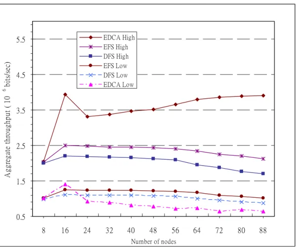
(39) 4.2 Simulation Results We evaluate the aggregate throughput of high priority flows by summarizing all the throughput of high priority flows and the aggregate throughput of low priority flows by summarizing all the throughput of low priority flows. We also evaluate the. fairness index [12]. We compare the proposed EFS with DFS and EDCA.. 4.2.1 Aggregate Throughput Fig. 8 shows the aggregate throughput for low and high priority stations versus the number of stations. Each high priority flow is assigned a weight of 8/3n and each low priority flow is assigned a weight of 4/3n. We can see that the EDCA’s aggregate throughput of high priority flows is higher than EFS and DFS. EDCA can achieve higher throughput because in the EDCA ns-2 implementation [13], it has implemented the Contention Free Burst (CFB). The EDCA can achieve much higher aggregate throughput with CFB than without CFB. We also can see that. the throughput. changes between 16 and 24 stations. The throughput degrades because in the case of 16 stations, there are 8 flows whose total offered load are 6 Mbps while in the case of 24 stations, there are 12 flows whose total offered load are 9 Mbps, which are greater than the real bandwidth limit of 11 Mbps in Wireless LAN. Thus, in the case of 24 stations, some time was wasted due to contention such as collision or choosing larger backoff intervals. In addition, the high priority flows get more and more throughputs because the low priority flows get less and less throughputs. EFS and DFS both can allocate bandwidth to flows in proportion to their weights. The proposed EFS can achieve higher aggregate throughput than DFS because the EFS effectively reduce idle slots using Division_Factor (DF) and can dynamically change the DF value according to the network load condition. Note that, the high priority flows of EDCA. 26.

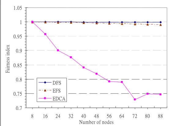
(40) get more and more aggregate throughput than the low ones with the increase of the number of stations. The EDCA results in unfairness between high and low priority flows.. EDCA High EFS High DFS High EFS Low DFS Low EDCA Low. 4.5. Aggregate throughput ( 10. 6. bits/sec). 5.5. 3.5. 2.5. 1.5. 0.5 8. 16. 24. 32. 40. 48. 56. 64. 72. 80. 88. Number of nodes. Fig. 8. The aggregate throughput of High and Low priority flows.. 4.2.2 Fairness Index and Throughput Variance For environments where all flows are always backlogged, we evaluate a fairness index [12] as follows:. fairness _ index =. (∑ f T f / φ f ) 2. number _ of _ flows × ∑ f (T f / φ f ) 2. 27. (16).

(41) where Tf denotes the throughput of flow f, and ψf denotes the weight of flow f. Remind that, the higher the value of the fairness index, the higher is the fairness. Fig. 9 shows that the fairness index achieved by EDCA degrades as the number of stations in the wireless LAN increases. This is because that as the number of stations increases, there is an increase of collisions. To be fair, colliding stations should get prior access over other stations after suffering a collision. However, in EDCA, the colliding nodes start binary exponential backoff to pick a larger backoff interval and hence do not get prior access over other stations. This results in unfairness towards the colliding nodes. On the other hand, the proposed EFS and the DFS achieve a high fairness index even when the number of stations increases.. 1.05 1. Fairness index. 0.95 0.9 0.85 0.8. DFS EFS. 0.75. EDCA. 0.7 8. 16. 24. 32. 40 48 56 Number of nodes. 64. 72. 80. 88. Fig. 9. The fairness index of different schemes.. Fig. 10 and 11 show the throughput achieved by each high priority flow and 28.

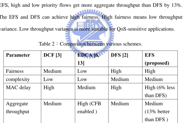
(42) each low priority flow. The X-axis represents the receiving station ID of each flow. We consider a scenario when there are sixty-four stations. We can see that flows with the same priority in the EDCA suffered from high throughput variance. The reason leading to this situation is just as the reason leading to unfairness, and randomness in choosing a backoff interval is also another significant factor. However, in DFS and EFS, flows with the same priority had low throughput variance. High throughput variance is undesired for time-sensitive applications. We solve this problem by assigned flows’ backoff intervals in proportion to their weights. Note that EFS has a little higher throughput variance than DFS due to the fast backoff mechanism. Table 2 summarizes the evaluation results by comparing various schemes. In the proposed EFS, high and low priority flows get more aggregate throughput than DFS by 13%. The EFS and DFS can achieve high fairness. High fairness means low throughput variance. Low throughput variance is more suitable for QoS-sensitive applications. Table 2：Comparison between various schemes. Parameter. DCF [3]. EDCA [6, 13]. DFS [2]. EFS (proposed). Fairness. Medium. Low. High. High. complexity. Low. Low. Medium. Medium. MAC delay. High. Medium. High. High (6% less than DFS). Aggregate throughput. Medium. High (CFB enabled ). Medium. Medium (13% better than DFS ). 29.

(43) 0.35. EDCA High EFS High DFS High. Throughput ( M bits/s ). 0.3. 0.25. 0.2. 0.15. 0.1 1. 5. 9. 13 17 21 25 29. 33 37 41 45 49 53 57 61. Station ID. Fig. 10. The throughput obtained by each high priority station (flow).. 0.08. Throughput (M bits/s). 0.07 0.06 0.05 0.04 0.03 EFS Low. 0.02. DFS Low EDCA Low. 0.01 3. 7. 11 15 19 23 27 31 35 39 43 47 51 55 59 63 Station ID. Fig. 11. The throughput obtained by each low priority station (flow).. 30.

(44) 4.2.3 MAC Delay We also evaluate the average MAC delays of the EFS, DFS, and EDCA. The average MAC delay is computed by summarizing the MAC delay of all the packets and averaging it. The results are shown in Fig. 12. We can see that EFS slightly reduce the average MAC delay compared to DFS since we have enhanced the DFS by reducing idle time slots and enhanced the collision handling of the DFS. As shown in equation (6), the value of DF can determine the rate of reducing idle time slots. The EFS and DFS both have higher average MAC delay than the EDCA due to the use of contention free bursting in EDCA. Since the EFS and DFS choose a backoff interval for each packet with consideration of fair scheduling, this results in longer average MAC delay than the EDCA.. 80. Average MAC delay (ms). 70 60 50. DFS. 40. EFS EDCA. 30 20 10 0 8. 16. 24. 32. 40. 48. 56. 64. 72. Number of stations. Fig. 12. The average MAC delay of different schemes 31. 80.

(45) Chapter 5 Conclusions and Future Work 5.1 Concluding Remarks We have proposed the Enhanced Fair Scheduling (EFS) for supporting weighted fair scheduling in IEEE 802.11e wireless LANs. The goal of the EFS is to achieve a fair allocation of bandwidth and to enhance the throughput performance. In the EFS, a packet with the smallest ratio between its length and weight receives the highest priority to transmit. The main idea of this scheme is to pick a backoff interval proportional to the finish tag of the packet. By picking a right backoff interval and using appropriate collision resolution in the transmission failure state, we can achieve fair allocation of bandwidth. With the fast backoff mechanism in the backoff timer decrement state and by dynamically adjusting the backoff interval according to the network load, we can enhance the performance of EFS. Simulation results have shown that the proposed EFS can achieve 13% higher throughput, 6% lower delay than DFS. Both have nearly equal fairness indexes, which mean both can allocate bandwidth to the flows in proportion to their weights. However, the EFS suffers from a little higher throughput variability than DFS due to the fast backoff mechanism.. 5.2 Future Work In the future, we will dynamically modify other parameters for the proposed EFS, such as Scaling_Factor, according to the network load and application requirements.. 32.

(46) We can also study the impact of adjusting Backoff Threshold and Division_Factor. The Contention Free Burst (CFB) mechanism in EDCA is good for throughput performance but is harmful for fairness. We will research how to incorporate the CFB mechanism into our EFS to further enhance throughput and delay performance, and will not sacrifice fairness.. 33.

(47) Bibliography [1] M. Shreedhar and G. Varghese, “Efficient fair queuing using deficit round-robin,” IEEE/ACM Transactions on Networking, vol. 4, no. 3, pp. 375-385, 1996. [2] N. H. Vaidya, P. Bahl, and S. Gupta, “Distributed fair scheduling in a wireless LAN,” in Proc. Mobile Computing and Networking Conference, 2000, pp. 167-178.. [3] IEEE and. standard Physical. for Layer. wireless (PHY). LAN. medium. specifications,. access. control (MAC). ISO/IEC 8802-11: 1999 (E),. Aug. 1999.. [4] S. Choi, J. del Prado, N. Sai Shankar, and S. Mangold, “IEEE 802.11e contention-based channel access (EDCF) performance evaluation,” in Proc. IEEE International Conference on Communications, May 2003, pp. 1151-1156,.. [5] I. Aad and C. Castelluccia, “Differentiation mechanisms for IEEE 802.11,” in Proceedings of IEEE INFOCOM, Anchorage, Alaska, April 2001.. [6] IEEE WG, “802.11e draft 3.1,” May 2002.. 34.

(48) [7] S. J. Golestani, “A self-clocked fair queueing scheme for broadband applications,” in IEEE INFOCOM, 1994, pp.636-646.. [8] W. Pattara-atikom, S. Banerjee and P. Krishnamurthy, “Starvation prevention and quality of service in wireless LANs,” in Proc. IEEE Wireless Personal Multimedia Communication, Oct. 2002, vol. 3, pp.1078-1082.. [9] Network Simulator document. [Online]. Available: http://www.isi.edu/nsnam/ns 2002.. [10] Y. Kwon, Y. Fang, and H. Latchman, “Fast collision resolution (FCR) MAC algorithm for wireless local area networks,” in Proc. Global Telecommunications Conference, Nov. 2002, vol. 3, pp. 2250-2254.. [11] L. Romdhani, Q. Ni and T. Turletti, “Adaptive EDCF: enhanced service differentiation for IEEE 802.11 wireless ad hoc networks,” in Proc. IEEE Wireless Communication and Networking, March 2003, vol. 2, pp. 1373-1378.. [12] R. Jain, A. Durresi, and G. Babic, “Throughput fairness index: an explanation,” ATM Forum/99-0045, Feb. 1999. [13] An IEEE 802.11e EDCF and CFB simulation model for NS-2.26 [Online]. Available: http://www.tkn.tu-berlin.de/research/802.11e_ns2/. 35.

(49) [14] W. Pattara-Atikom, P. Krishnamurthy, and S. Banerjee, “Distributed mechanisms for quality of service in wireless LANs, ” IEEE Wireless Communications vol. 10, no. 3, pp. 26-34, June 2003. [15] A. Lindgren, A. Almquist, and O. Schelen, “Evaluation of quality of service schemes for IEEE 802.11 wireless LANs,” in Proc. IEEE Local Computer Networks, Nov. 2001, pp. 348-351.. [16] D. He and C.Q. Shen, “Simulation study of IEEE 802.11e EDCF,” in Proc. IEEE Vehicular Technology Conference, April 2003, vol. 1, pp. 685-689.. [17] G. W. Wong, and R. W. Donaldson, “Improving the QoS performance of EDCF in IEEE 802.11e wireless LANs,” in Proc. IEEE Communications, Computers and Signal Processing Conference, Aug 2003, vol. 1, pp. 392-396.. [18] A. K. Parekh and R. G. Gallager, “A generalized processor sharing approach to flow control in integrated services networks: the single-node case,” IEEE/ACM Transactions on Networking, vol. 1, pp. 344-357, June 1993.. [19] P. Goyal, H. M. Vin, and H. Cheng, “Start-time fair queuing: a scheduling algorithm for integrated serivces switched networks,” IEEE/ACM Transactions on Networking, vol. 5, pp. 690–704, October 1997.. 36.

(50) [20] T. Nandagopal, S. Lu, and V. Bharghavan, “A unified architecture for the design and evaluation of wireless fair queuing algorithms,” in Proceedings of ACM MOBICOM, Seattle, WA, August 1999, pp. 132-142.. [21] V. Kanodia, C. Li, B. Sadeghi, A. Sabharwal, and E. Knightly, “Distributed multi-hop with delay and throughput constraints,” in Proceeding of MOBICOM, Rome,Italy, July 2001, pp. 200-209.. [22] J. C. R. Bennett and H. Zhang, “Wf2q: worst-case fair weighted fair queueing,” in Proc. IEEE INFOCOM, March 1996, pp. 120-128.. 37.

(51)