應用多重區域條件式成組縮放法於快速傅利葉
轉換處理器之面積最小化技術
Area Minimization for FFT Processor Using Multi-Region
Conditional Block Scaling
研 究 生:陳柏霖 Student:Po-Lin Chen
指導教授:周景揚 Advisor:Jing-Yang Jou
國 立 交 通 大 學
電子工程學系 電子研究所
碩 士 論 文
A ThesisSubmitted to Department of Electronics Engineering and Institute of Electronics College of Electrical and Computer Engineering
National Chiao Tung University In Partial Fulfillment of the Requirements
for the Degree of Master of Science
in
Electronics Engineering
September 2012
Hsinchu, Taiwan, Republic of China
I
應用多重區域條件式成組縮放法於快速傅利葉轉換處理器
之面積最小化技術
學生:陳柏霖
指導教授:周景揚 博士
國立交通大學
電子工程學系 電子研究所碩士班
摘 要
快速傅利葉轉換處理器是正交分頻多工系統的計算核心,並且在過去幾十年間可以 找到許多研究資料。為了提升定字元長度傅利葉轉換處理器的訊號對量化雜訊比,動態 縮放法在執行運算時適應性地決定其縮放行為以避免不必要的精確度流失。當訊號對量 化雜訊比的要求提高時,傳統上是去增加字元長度以得到更高的精確度。然而增加字元 長度在面積上會付出許多代價,再者,有時候其實並不需要將精確度提升這麼多去滿足 要求。在這篇論文裡,我們提出了一個利用了條件式縮放法及成組縮放法的優點的動態 縮放法。此方法擁有非常經濟地使用面積去提升訊號對量化雜訊比的能力而不只是單純 地去增加字元長度。因此,此方法的目標是在滿足訊號對量化雜訊比的要求下得到最小 化的快速傅利葉轉換處理器的面積。實驗結果顯示在最佳的情形下,我們的方法相較於 原本的條件式縮放法可以對 8192 點的快速傅利葉轉換處理器省下約 13% 的面積。II
Area Minimization for FFT Processor Using Multi-Region
Conditional Block Scaling
Student:Po-Lin Chen
Advisor:Dr. Jing-Yang Jou
Department of Electronics Engineering
Institute of Electronics
National Chiao Tung University
ABSTRACT
The Fast Fourier Transform (FFT) processor is the key component of OFDM-base systems, and many literatures of FFT can be found in the past decades. To improve the SQNR in fixed-wordlength FFT, dynamic scaling methods adaptively determine the scaling behavior in run time to avoid the unnecessary loss of data information. Traditionally, increasing the wordlength is the way to acquire higher precision if the SQNR constraint is tighter. However, the increased wordlength results in a large amount of area cost. Moreover, sometimes we do not have to increase SQNR so much to meet the constraint. In this thesis, we proposed a dynamic scaling scheme which utilizes the profits of conditional scaling method and block scaling method. Our approach has the ability to economize the usage of area rather than increase the wordlength for SQNR improvement and the target is to minimize the area of FFT under the SQNR constraint. Experimental results show that our approach can reduce the area cost by about 13% in the best case for 8192-point FFT as compared to the existing conditional scaling method.
III
Acknowledgements
I would like to express my sincere gratitude to my advisors, Dr. Jing-Yang Jou for his patient guidance and valuable suggestion during these years. I am also grateful to Dr. Juinn-Dar Huang for his help on my research. Besides, I have many thanks to my seniors Bu-Ching Lin, Yung-Chun Lei and my lab-mate Chuang-Ren Yang for their gentle teaching, directing, and beneficial discussion. Moreover, I greatly appreciate all members of NCTU EDA Lab. All of you are so nice that I will remember the happy time during the past two years with you. Finally, I wish to give my deepest acknowledgements to my family and my girlfriend, Pei-Chen Wu for their love, support, and encouragement.
IV
Contents
摘 要………...………..I ABSTRACT ... II Acknowledgements ... III Contents………IV List of Figures ... VI List of Tables ... VIIIChapter 1 Introduction ... 1
Chapter 2 Preliminaries ... 4
2.1 The FFT Algorithms ... 4
2.1.1 Basic Concepts of FFT Algorithms ... 4
2.1.2 Radix-2 DIT FFT Algorithm ... 6
2.1.3 Radix-4 DIT FFT Algorithm ... 8
2.1.4 Radix-r DIT FFT Algorithm ... 9
2.2 The FFT Architectures... 9 2.2.1 Memory-Based Architectures ... 9 2.2.2 Pipeline-Based Architectures ... 10 2.3 Scaling Operation ... 11 2.4 Scaling Method ... 14 2.4.1 Forced Scaling ... 14
2.4.2 Block Floating Point Scaling ... 15
2.4.3 Conditional Scaling ... 17
Chapter 3 Motivation ... 20
3.1 Multi-Region Detection ... 20
3.2 Convergent Block Scaling ... 21
3.3 Our Strategy ... 23
V
Chapter 4 The Proposed Approach ... 24
4.1 Scheduling of Butterfly Computation... 24
4.2 Multi-Region Conditional Block Scaling ... 25
4.2.1 Region Detector ... 27
4.2.1.1 Circular-Type Detector ... 27
4.2.1.2 Square-Type Detector ... 31
4.2.2 Overflow Predictor ... 33
4.2.3 Exponent Unit ... 36
4.3 Restricted Number of Blocks ... 38
Chapter 5 Experimental Results ... 40
5.1 The Solution Generated by MRCBS ... 41
5.1.1 Performance Pair of the Forced Scaling FFT ... 42
5.1.2 Improvement from Multi-Region Detection... 42
5.1.3 Improvement from Convergent Block Scaling ... 43
5.1.4 Performance Pair Combination ... 45
5.2 Area Minimization under SQNR Constraint ... 47
Chapter 6 Conclusions and Future Works ... 50
VI
List of Figures
Fig. 1 Simplified architecture of OFDM system ... 1
Fig. 2 Symmetric property of twiddle factor ... 5
Fig. 3 First stage of the DIT FFT algorithm for 8-point FFT... 6
Fig. 4 The butterfly unit of a radix-2 DIT FFT algorithm... 7
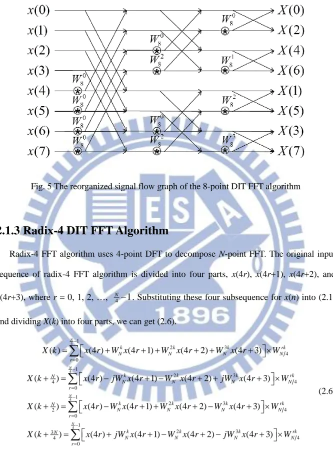
Fig. 5 The reorganized signal flow graph of the 8-point DIT FFT algorithm ... 8
Fig. 6 A simple architecture of memory-based FFT ... 10
Fig. 7 The R2SDF architecture for 16-point pipeline-based FFT ... 11
Fig. 8 An example of scaling operation ... 12
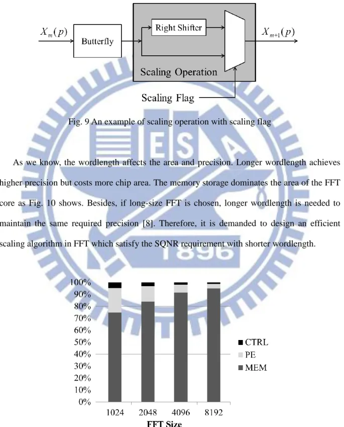
Fig. 9 An example of scaling operation with scaling flag ... 13
Fig. 10 The area occupancy of each component in memory-based 16-bit FFT ... 13
Fig. 11 The architecture of the forced scaling method ... 14
Fig. 12 Floating point representation ... 15
Fig. 13 An example of 8-point FFT with 4 blocks BFP scaling ... 16
Fig. 14 A data block example with block size = 4 ... 16
Fig. 15 The architecture of the BFP scaling method ... 16
Fig. 16 The architecture of the conditional scaling method ... 17
Fig. 17 The particular region of the complex plane in conditional scaling method ... 18
Fig. 18 The complex plane with (a) two regions (b) four regions are divided ... 21
Fig. 19 An example of 8-point FFT with convergent block scaling ... 22
Fig. 20 Detection of the two data in the same butterfly of next stage ... 25
Fig. 21 The architecture of the proposed MRCBS ... 26
Fig. 22 The regions of the circular-type detectors (a) C2 (b) C4 (c) C6 ... 28
Fig. 23 The simulation result of SQNR with different t-1 ... 30
Fig. 24 The block diagram of the circular-type detector ... 30
Fig. 25 The regions of the square-type detectors (a) S2 (b) S4 (c) S6... 32
Fig. 26 The simulation result of SQNR with different h-1 ... 32
Fig. 27 The block diagram of the square-type detector ... 33
Fig. 28 Overflow Prediction based on the region information of the inputs... 34
Fig. 29 The block diagram of the overflow predictor ... 35
Fig. 30 The exponent array with the exponent unit ... 36
VII
Fig. 32 The usage of the exponent array for convergent block scaling with 8 blocks ... 37
Fig. 33 The convergent block scaling with (a) Bmax = 1 (b) Bmax = 2 (c) Bmax = 4 ... 38
Fig. 34 The SQNR and area cost with different Bmax ... 39
Fig. 35 The PPTs for 1024-point FFT generated by MRCBS ... 46
Fig. 36 The PPTs for 2048-point FFT generated by MRCBS ... 46
Fig. 37 The PPTs for 4096-point FFT generated by MRCBS ... 47
VIII
List of Tables
Table 1 The value of the thresholds in circular-type detectors ... 29
Table 2 The value of the thresholds in square-type detectors ... 31
Table 3 The value of region information P and Q according to the data locations ... 34
Table 4 Scaling decision according to the summation of P and Q ... 35
Table 5 The PPBase determined by (N, WL) (a)SQNRBase (dB) (b)AREABase (µm2) ... 42
Table 6 The SQNRx(dB) of the PPxfor (a)1024 (b)2048 (c)4096 (d)8192 -point FFT ... 43
Table 7 The AREAx(µm2) of the PPx ... 43
Table 8 The PPy (dB, µm2) for (a) 1024 (b)2048 (c)4096 (d) 8192 -point FFT ... 45
Table 9 The solutions under the SQNR constraints for 1024-point FFT ... 48
Table 10 The solutions under the SQNR constraints for 2048-point FFT ... 49
Table 11 The solutions under the SQNR constraints for 4096-point FFT ... 49
1
Chapter 1
Introduction
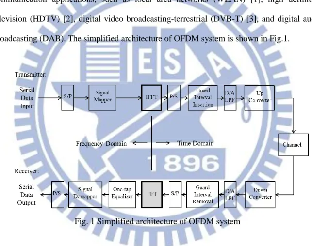
In recent years, research and development on high-data-rate wireless communications have attracted great attention. Orthogonal frequency-division-multiplexing (OFDM) is the modulation technique which is a favorable choice for many new and emerging broadband communication applications, such as local area networks (WLAN) [1], high definition television (HDTV) [2], digital video broadcasting-terrestrial (DVB-T) [3], and digital audio broadcasting (DAB). The simplified architecture of OFDM system is shown in Fig.1.
Fig. 1 Simplified architecture of OFDM system
In those applications, Fast Fourier Transform (FFT) is the most widely used algorithms for calculating the Discrete Fourier Transform (DFT) because of its efficiency in reducing computation time. Therefore, it is one of the most important processing blocks to meet the design constraints. In [4], the authors showed that in such high-data-rate systems, the most computationally intensive part is the FFT core. Therefore, there have been many literatures reported on the design of FFT processors nowadays.
2
Based on the hardware cost and the required throughput, there are two main categories of FFT architectures. One is called memory-based architectures, which consist of a butterfly unit and certain number of memory blocks. The other is called pipeline-based architecture, which consists of multiple stages to provide higher throughput. In general, memory-based architectures are suitable for long-size and low hardware design [5]. And pipeline-based architectures are feasible for short-size and high throughput design. In this thesis, we focus on the long-size FFT design with memory-based architecture where the wordlength WL of the output in every stage is the same as that of the input.
Taking the practical design into consideration, the precision of FFT module in terms of Signal to Quantization Noise Ratio (SQNR) is a significant design factor of system performance. In reality, an FFT cannot be implemented exactly since the algorithm is implemented by fixed-point arithmetic. All signals and coefficients have to be represented with finite number of bits in binary format. Therefore, conducting the addition and subtraction operations in butterfly unit may cause overflow during the FFT computations. For this reason, the wordlength should be increased stage by stage to avoid possible overflow after butterfly computations. The increasing wordlength can be used to avoid accuracy loss and increase the precision [6], but the hardware cost and the critical-path delay are increased accordingly and it is unsuitable for memory-based architecture. Consequently, rounding or truncation operations introduce noise which is referred as quantization noise and result in accuracy loss. Furthermore, the wordlength may also affect the accuracy. Longer wordlength may be used to achieve better SQNR with larger area, and shorter wordlength may be chosen to maintain a lower hardware cost at the sacrifice of the precision. Therefore, many scaling methods have been proposed to meet SQNR requirement with the fixed-wordlength constraint [7-12].
Oppenheim et al. [7] proposed a basic scaling method which scales the results by a factor of 1/2 for each stage. That is, the results are divided by two after each butterfly calculation. Since it is trivial to implement, the approach is the simplest but the least accurate scaling
3
method called the forced scaling method. Another is called the Block Floating Point (BFP) scaling [11] which employs intermediate buffers to store the output data, and detects the largest value to decide the output format appropriately which gets better SQNR. However, this kind of method results in a large amount of area overhead and power consumption. Besides, there is another approach which is called conditional scaling [13, 14]. The idea of the method is to predetermine whether to scale in next stage according to the magnitude of the results in current stage. That is to say, after each butterfly computation, the magnitudes of the results are compared to a threshold and the results can be written back to the memory instantly after the comparisons. After all comparisons are finished, it will be judged that overflow will occur in next stage if one or more values exceed 0.5. Thus, after each computation of the butterfly in next stage, the results will be scaled to avoid overflow. Although the conditional scaling method acquires less SQNR than BFP, it saves much area since it does not need the buffers to store internal results.
In this thesis, we propose a dynamic scaling method combining the concepts of BFP scaling and conditional scaling with memory-based architecture to acquire higher SQNR in an area-efficient way. Our method not only improves the previous conditional scaling method to predict overflow more precise but also modifies BFP scaling to divide data into blocks appropriately. Moreover, our method can minimize the area with given FFT size and SQNR constraint.
The remainder of this thesis is organized as follows. In Chapter 2, we briefly review the fundamentals of FFT algorithms, architectures and previous scaling methods. Chapter 3 explains the motivation of this work. The proposed method is demonstrated in Chapter 4. Our experimental results are shown in Chapter 5. Finally, Chapter 6 gives the concluding remarks of this thesis.
4
Chapter 2
Preliminaries
In this chapter, we will review basic FFT algorithms, FFT architectures, the scaling considerations and previous scaling methods in FFT hardware design.
2.1 The FFT Algorithms
The Discrete Fourier Transform (DFT) plays an important role in the region of digital signal processing (DSP) and communications. However, the computation complexity of directly evaluating an N-point DFT is O(N2), which costs a lot amount of computation time and power consumption. Therefore, a fast algorithm to evaluate DFT is required.
FFT algorithm is a decomposition of an N-point DFT into successively smaller DFT transform which was proposed by Cooley and Turkey [15] in 1965. It is very popular because it reduces the complexity of DFT from O(N2) to O N( log2N), and makes it suitable for VLSI implementation due to the regularity of the algorithm. Besides, many similar algorithms have been developed to further reduce the computational complexity of FFT [16-18]. Owing to these algorithms, FFT computes the DFT efficiently and produces exactly the same result as evaluating the DFT equation.
2.1.1 Basic Concepts of FFT Algorithms
FFT algorithms are approaches to evaluate DFT. The formulation of N-point DFT is defined as 1 0 ( ) ( ) , 0, 1, ..., 1 N nk N n X k x n W k N
(2.1)5
Where X(k), x(n) and WNnk are complex numbers. X(k) is in frequency domain, and x(n) is in
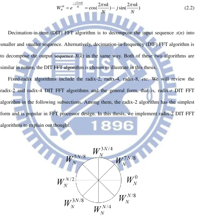
time domain. The coefficient WNnk is defined as (2.2) and is called the twiddle factor which the symmetric property is shown in Fig. 2.
2 2 2 cos( ) sin( ) j nk nk N N nk nk W e j N N (2.2)
Decimation-in-time (DIT) FFT algorithm is to decompose the input sequence x(n) into smaller and smaller sequence. Alternatively, decimation-in-frequency (DIF) FFT algorithm is to decompose the output sequence X(k) in the same way. Both of these two algorithms are similar in nature, the DIT FFT algorithm is chosen to illustrate in this thesis.
Fixed-radix algorithms include the radix-2, radix-4, radix-8, etc. We will review the radix-2 and radix-4 DIT FFT algorithms and the general form, that is, radix-r DIT FFT algorithm in the following subsections. Among them, the radix-2 algorithm has the simplest form and is popular in FFT processor design. In this thesis, we implement radix-2 DIT FFT algorithms to explain our thought.
6
2.1.2 Radix-2 DIT FFT Algorithm
The raidx-2 algorithm is using the divide-and-conquer approach which divides the problem of N-point FFT by a factor of 2, where N is power-of-2. Radix-2 DIT FFT Algorithm divides x(n) into its even-numbered points and odd-numbered points, and uses 2r to substitute n for n is even, 2r+1 to substitute n for n is odd.
2 2 2 2 1 1 2 1 2 0 0 1 1 2 2 0 0 ( ) (2 ) (2 1) (2 ) (2 1) N N N N r k rk N N r r rk k rk N N N r r X k x r W x r W x r W W x r W
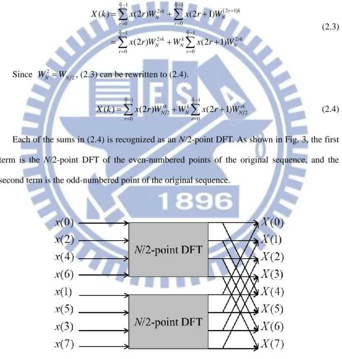
(2.3)Since WN2 WN2, (2.3) can be rewritten to (2.4). 2 1 2 1 2 2 0 0 ( ) (2 ) (2 1) N N rk k rk N N N r r X k x r W W x r W
(2.4)Each of the sums in (2.4) is recognized as an N/2-point DFT. As shown in Fig. 3, the first term is the N/2-point DFT of the even-numbered points of the original sequence, and the second term is the odd-numbered point of the original sequence.
7
Then we divide the original k into two new parts k and kN2 , for k = 0, 1, …,
2 1 N . Since 2 2 /2 1 N N j N j N
W e e and WNr N 2 WNrWNN/2 WNr, (2.4) can be rewritten to (2.5). Through log2N-time recursive decompositions, the complete radix-2 DIT FFT algorithm
can be obtained. 2 1 2 0 ( ) ( 2 ) ( 2 1 ) N k r k N N r X k x r W x r W
2 1 2 0 ( ) (2 ) (2 1) 2 N k rk N N r N X k x r W x r W
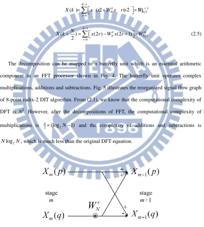
(2.5)The decomposition can be mapped to a butterfly unit which is an essential arithmetic component in an FFT processor shown in Fig. 4. The butterfly unit operates complex multiplications, additions and subtractions. Fig. 5 illustrates the reorganized signal flow graph of 8-point radix-2 DIT algorithm. From (2.1), we know that the computational complexity of DFT is N2. However, after the decompositions of FFT, the computational complexity of multiplications is N2 (log2N1) and the complexity of additions and subtractions is
2
log
N N , which is much less than the original DFT equation.
8
Fig. 5 The reorganized signal flow graph of the 8-point DIT FFT algorithm
2.1.3 Radix-4 DIT FFT Algorithm
Radix-4 FFT algorithm uses 4-point DFT to decompose N-point FFT. The original input sequence of radix-4 FFT algorithm is divided into four parts, x(4r), x(4r+1), x(4r+2), and x(4r+3), where r = 0, 1, 2, …, N4 1. Substituting these four subsequence for x(n) into (2.1) and dividing X(k) into four parts, we can get (2.6).
4 4 4 1 2 3 4 0 1 2 3 4 4 0 1 2 3 2 0 ( ) (4 ) (4 1) (4 2) (4 3) ( ) (4 ) (4 1) (4 2) (4 3) ( ) (4 ) (4 1) (4 2) (4 3) N N N k k k rk N N N N r k k k rk N N N N N r k k k N N N N r X k x r W x r W x r W x r W X k x r jW x r W x r jW x r W X k x r W x r W x r W x r W
4 4 1 2 3 3 4 4 0 ( ) (4 ) (4 1) (4 2) (4 3) N rk N k k k rk N N N N N r X k x r jW x r W x r jW x r W
(2.6)Although the complexity of multiplications in the radix-4 FFT algorithm is equal to
3
4
4N(log N1), which is lower than radix-2, the complexity of additions and subtractions is
9
2.1.4 Radix-r DIT FFT Algorithm
Larger r can much further reduce the complexity of multiplications. For general cases, we derive the radix-r DIT FFT algorithm, where r is 2S, and S is any positive integer. For N-point FFT, the general form is
1 1 0 0 ( ) ( ) N r r pq pk nk r N N r p n qN X k W W X rn p W r
(2.7)where q = 0, 1, …, r-1. And the complexity of multiplications is (SS1)N(logS N1).
2.2 The FFT Architectures
The FFT is one of the most widely used DSP algorithms. Generally speaking, there are two kinds of popular FFT architectures to implement FFT algorithms. One is memory-based architectures and the other is pipeline-based architectures. Memory-based architectures are suitable for low throughput, low hardware cost, and long-size FFT designs whose size is not smaller than 512 [5]. On the other hand, pipeline-based architectures are suitable for high throughput, high hardware cost and short-size FFT designs. In this thesis, we focus on long-size FFT design with memory-based architecture. The details of those two architectures are introduced in the following subsections.
2.2.1 Memory-Based Architectures
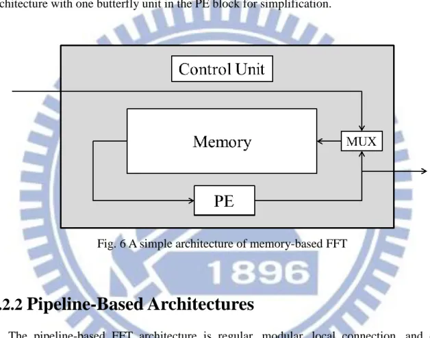
The memory-based architecture is the simplest FFT architecture. It consists of one memory device and one radix-r processing element (PE) which contains one or few butterfly units to operate all computations in the signal flow graph. The basic components of memory-based architecture are shown in Fig. 6. Data are read from the memory and computed in the PE. After the computations, the output data are written back to the memory
10
and occupy the same storage locations as input data. For radix-2 FFT algorithm, there are
2
log N stages for the N-point FFT computations, and the number of butterflies in the PE can be chosen freely to meet the throughput rate requirement. The generalized conflict-free addressing schemes for memory-based FFT architectures presented in [19, 20] solve the problem of the memory bandwidth. In this work, we implement the memory-based FFT architecture with one butterfly unit in the PE block for simplification.
Fig. 6 A simple architecture of memory-based FFT
2.2.2
Pipeline-Based Architectures
The pipeline-based FFT architecture is regular, modular, local connection, and often adopted for high-throughput-rate applications with high hardware complexity [21]. It can be generally divided into two kinds of architectures depending on the design of register. One is the Single-path Delay Feedback (SDF) architecture [22, 23] and the other is the Multi-path Delay Commutator (MDC) architecture [24]. SDF architecture has higher hardware usage and lower hardware cost. On the other hand, MDC architecture has higher throughput than SDF architecture. Here we only introduce the radix-2 SDF architecture as below since we do not take the pipeline-based architecture into account in this work.
11
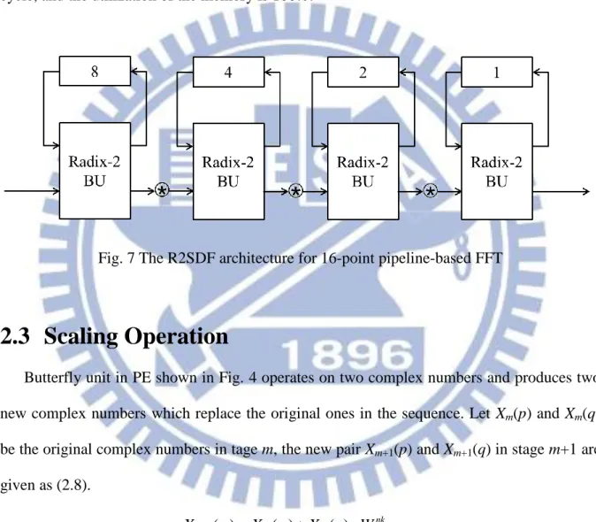
Take the radix-2 SDF (R2SDF) architecture as an example and the architecture is shown in Fig. 7. The R2SDF uses the registers efficiently by storing the output of the butterfly into the shift registers. When doing addition operation, the butterfly unit passes the output to the next stage. On the contrary, the butterfly unit stores the output into the shift registers when doing subtraction operation. Thus, there is only one output passes to the next stage in each cycle, and the utilization of the memory is 100%.
Fig. 7 The R2SDF architecture for 16-point pipeline-based FFT
2.3 Scaling Operation
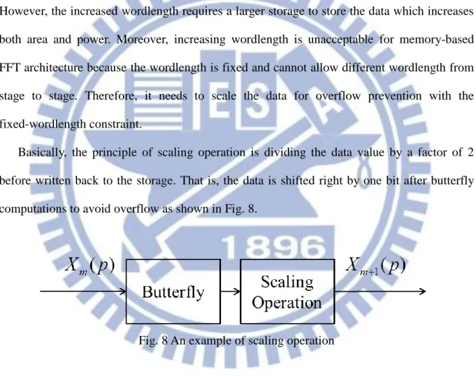
Butterfly unit in PE shown in Fig. 4 operates on two complex numbers and produces two new complex numbers which replace the original ones in the sequence. Let Xm(p) and Xm(q)
be the original complex numbers in tage m, the new pair Xm+1(p) and Xm+1(q) in stage m+1 are
given as (2.8). 1 1 ( ) ( ) ( ) ( ) ( ) ( ) nk m m m N nk m m m N X p X p X q W X q X p X q W (2.8)
The coefficient WNnk is the twiddle factor and substantially is the complex root of unity. For this reason, (2.9) shows that the multiplication with twiddle factor in the butterfly does not change the magnitude of the result. Hence, the magnitude of outputs can never be larger than twice the maximum magnitude of inputs as (2.10) explains.
12 ( ) nk ( ) nk ( ) m N m N m X q W X q W X q (2.9)
1( ) ( ) ( ) ( ) ( ) 2 max ( ) , ( ) nk m m m N m m m m X p X p X q W X p X q X p X q (2.10)From (2.10), we know that the range of data is increased from stage to stage. Thus, there is possibility of overflow during computation of butterflies if the data wordlength does not increase. Naturally, increasing the wordlength is a solution to avoid possible overflow [6]. However, the increased wordlength requires a larger storage to store the data which increases both area and power. Moreover, increasing wordlength is unacceptable for memory-based FFT architecture because the wordlength is fixed and cannot allow different wordlength from stage to stage. Therefore, it needs to scale the data for overflow prevention with the fixed-wordlength constraint.
Basically, the principle of scaling operation is dividing the data value by a factor of 2 before written back to the storage. That is, the data is shifted right by one bit after butterfly computations to avoid overflow as shown in Fig. 8.
Fig. 8 An example of scaling operation
However, the truncation in scaling operation introduces noise and influences the accuracy. Longer wordlength will be needed to meet the required performance. As a result, the decision of whether to scale affects the accuracy very much. As shown in Fig. 9, a one-bit scaling flag is being defined to decide whether to truncate the least significant bit of the result or not. If the scaling flag is set to one, the result of the butterfly will be scaled. Otherwise, the result
13
keeps its original value without scaling. When the scaling operation is finished, results are written back to the memory device.
Fig. 9 An example of scaling operation with scaling flag
As we know, the wordlength affects the area and precision. Longer wordlength achieves higher precision but costs more chip area. The memory storage dominates the area of the FFT core as Fig. 10 shows. Besides, if long-size FFT is chosen, longer wordlength is needed to maintain the same required precision [8]. Therefore, it is demanded to design an efficient scaling algorithm in FFT which satisfy the SQNR requirement with shorter wordlength.
14
2.4 Scaling Method
The scaling method with a constant scaling flag of each stage is called static scaling method such as forced scaling [7] where the scaling flag is always set to one. Conversely, the scaling method determining the scaling factor of each stage at run-time is called dynamic scaling method, like BFP scaling [12] and conditional scaling [13, 14]. Each kind of scaling method has its advantages and disadvantages respectively. Static scaling is the simplest in hardware implementation as well as dynamic scaling greatly improves accuracy by ultimately avoiding unnecessary truncations. We will introduce these scaling schemes in fixed-wordlength FFT design as follows.
2.4.1 Forced Scaling
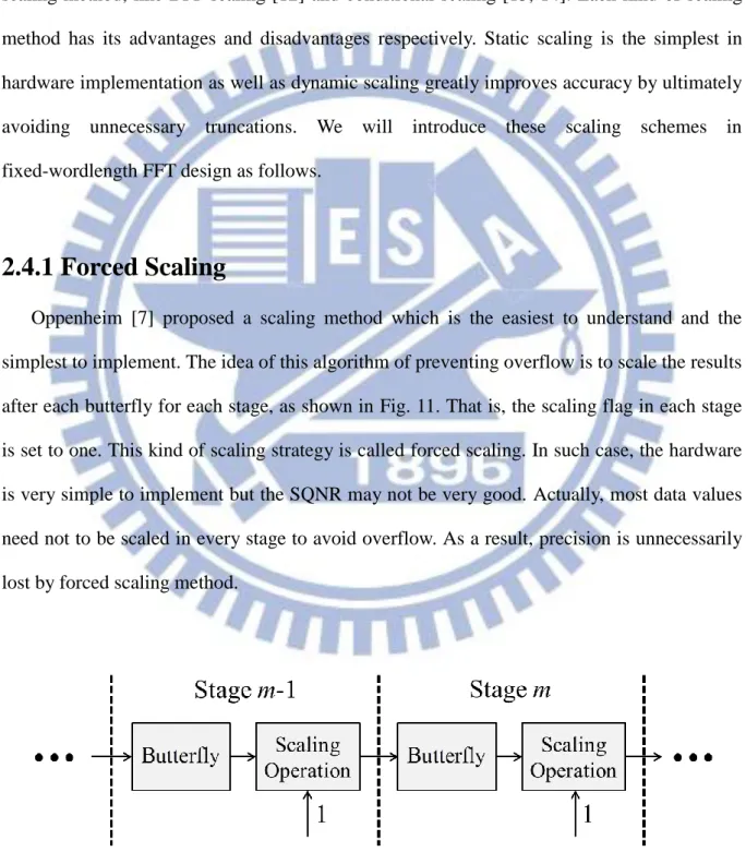
Oppenheim [7] proposed a scaling method which is the easiest to understand and the simplest to implement. The idea of this algorithm of preventing overflow is to scale the results after each butterfly for each stage, as shown in Fig. 11. That is, the scaling flag in each stage is set to one. This kind of scaling strategy is called forced scaling. In such case, the hardware is very simple to implement but the SQNR may not be very good. Actually, most data values need not to be scaled in every stage to avoid overflow. As a result, precision is unnecessarily lost by forced scaling method.
15
2.4.2 Block Floating Point Scaling
The floating point representation is shown in Fig. 12. The bit width of the floating point contains exponent bits, mantissa bits, and one sign bit. The magnitude of the value which is stored in the mantissa part is always smaller than one, and the value in the exponent part is an integer which is larger or equal to zero. BFP scaling method [12] uses a shared-exponent concept which groups the floating-point data into blocks with a common exponent to reduce the wordlength. An example of BFP with four blocks is shown in Fig. 13 where the capital letter “E” stands for the shared exponent of each block. The data only keep their own sign bit and mantissa bits, and each block has its own shared exponent as shown in Fig. 14. And the block size and the number of blocks are fixed through all stages.
Fig. 12 Floating point representation
Compared to the regular scaling such as forced scaling, BFP acquires higher performance of SQNR by avoiding unnecessary loss of data information. The idea is to scale only if we found the necessity of that. Thus, BFP employs intermediate buffers to store the output data of a certain block, as shown in Fig. 15. After all data in this block are computed and stored into the buffer, a detector will detect them to find out the largest value. If the magnitude of the largest value is larger than one, the scaling flag of this block is set to one. Then all the data are scaled and written back to the memory as the shared exponent is increased by one. On the other hand, if the largest value does not cause overflow, scaling will not be performed. Therefore, the least significant bit for each data value is preserved.
16
Fig. 13 An example of 8-point FFT with 4 blocks BFP scaling
Fig. 14 A data block example with block size = 4
Fig. 15 The architecture of the BFP scaling method
Unlike the forced scaling, BFP scales data only when it is necessary. By adaptively determining the scaling flag to avoid accuracy loss, BFP acquires better precision than forced scaling method. Hence, BFP uses shorter wordlength to achieve the required SQNR and saves the area of memory device. Unfortunately, the inputs of the butterfly in BFP scaling method
17
will come from different data blocks, that is, their exponent may not be the same. Therefore, the floating point arithmetic of addition and subtraction operation needs an alignment unit to align two input data. It needs to shift the mantissa bits to represent them with the same exponent. Since the exponent bits have to be checked and mantissa bits have to be shifted, it will be more complicated than fixed point arithmetic in hardware implementation. Moreover, the buffer accesses and data detections introduce the additional processing latency and power consumption. Also, the intermediate buffers, detectors and the storage of shared exponents cause a large amount of additional area overhead.
2.4.3 Conditional Scaling
Instead of storing results in the buffers and detecting the largest value to decide the scaling flag, the conditional scaling method using the concept of prediction is another way to avoid overflow but saves the area overhead of buffers. Fig. 16 shows the architecture of conditional scaling method. In details, conditional scaling predetermines the scaling flag of current stage by the detections in previous stage. Then the detections in current stage will predetermine the scaling flag of next stage. Therefore, conditional scaling does not need buffers to store intermediate results. Moreover, there is only one shared-exponent in conditional scaling because it uses the fixed point representation. As a result, the alignment unit is unnecessary. We can directly operate additions and subtractions on the two inputs of butterfly.
18
The criterion for deciding the scaling flag of next stage is based on the observation of whether any value in current stage is outside a particular region on the complex plane [13]. Besides, (2.10) tells us that Xm1( ) , p Xm1( )q Xm( )p Xm( )q . If Xm( )p and
( )
m
X q are both smaller than 0.5, Xm1( )p and Xm1( )q will be smaller than one.
Therefore, the region with which to compare the data in current stage is the circle of radius 0.5. As shown in Fig. 17, the circle of radius 0.5 is the idealized threshold for deciding the scaling flag of next stage.
Fig. 17 The particular region of the complex plane in conditional scaling method
The magnitudes of the results are checked during the butterfly computations. If all output data in current stage are inside the region with radius 0.5, it guarantees that there will not be any data with magnitude larger than one to cause overflow in next stage. Thus, the scaling flag will not be set and the exponent will be kept. On the contrary, if there is at least one data outside the circular region with radius 0.5, it may cause overflow through butterfly computation in next stage. As a result, when computing the butterflies of next stage, the results should be scaled and the exponent should be increased by one.
19
Because conditional scaling predicts the necessity of scaling, the SQNR performance of conditional scaling is much higher than that of forced scaling but a little lower than that of BFP scaling. However, calculating the magnitude of a complex number needs to compute the square of real part and imaginary part. The required multipliers and adders will cost area. Alternatively, for hardware concern, the maximal cyclic quadrilateral which is the square with dotted line in Fig. 17 is chosen to define the particular region [14]. As a result, only comparators are needed to detect the region information of data.
In this thesis, we will combine the concepts of BFP scaling method and the conditional scaling method and utilize the profits of them.
20
Chapter 3
Motivation
To satisfy the required SQNR performance, we will choose a scaling approach which produces SQNR higher enough with less area. However, once the constraint is tighter and the original design does not satisfy the requirement, using longer wordlength is the only way to further increase the accuracy. Based on the experience of simulations, increasing wordlength by one will acquire about 6 dB improvement for SQNR but about 6% area penalty in addition. However, sometimes we do not have to increase SQNR so much to meet the constraint. Thus, by the improvements of conditional scaling and modifications of block floating point scaling, we will acquire SQNR improvement in demand with the corresponding area overhead.
3.1 Multi-Region Detection
With the approaches of [13, 14], the complex plane has been divided into two regions to detect the region information of the outputs of the butterfly. Traditional conditional scaling method avoids overflow in current stage by ensuring the data in previous stage are all in the internal region with radius 0.5. However, overflow comes from the addition and subtraction operations in butterfly which result in the growth of data magnitude. And the computation only has relations with the two input data. That is to say, restricting all data in the same region to avoid overflow is excessively severe. In order to avoid overflow, we only need to ensure that Xm( )p Xm( )q is smaller than one as (2.10) says.
We assume that we are now computing butterflies in stage m-1, and the complex plane is divided into two regions as Fig. 18(a) shows. The Xm(q) is inside R0 and Xm(p) is outside R0
21
method, it is judged that overflow will be produced in stage m and the scaling flag of stage m will be set. However, overflow can also be avoided as long as Xm( )q is small enough. Therefore, we try to divide the complex plane into more regions. Fig. 18(b) shows the idea of which four regions are divided. In such case, Xm(p) is inside R+1 and Xm(q) is inside R-1 where
the radius of R+1 is 0.7 and the radius of R-1 is 0.2. By ensuring the summation of the radii of
R+1 and R-1 is less than unity, we can judge that the butterfly computation in stage m which
operates on these two data will not cause overflow. That is to say, dividing the complex plane into more regions will further prevent the unnecessary scaling operations and produce better SQNR performance. And we can expect that the more regions the complex plane is divided, the higher precision can be obtained.
(a) (b)
Fig. 18 The complex plane with (a) two regions (b) four regions are divided
3.2 Convergent Block Scaling
The hardware of floating point arithmetic is more complicated than that of fixed point arithmetic. As mentioned in 2.4.2, one part of the area overhead of BFP scaling method is the alignment unit because the floating point representation is used. Since the inputs of butterfly
22
may come from different blocks and their exponent may be different, we cannot operate these two mantissas directly without alignment. However, figuring out the larger exponent and shifting the smaller mantissa introduces area and processing latency. If we want to save the hardware of alignment unit, we must ensure that the two inputs of butterfly are come from the same block which means their exponent is always the same one.
It can be observed in Fig. 5 that during the decomposition of FFT algorithms, a k-point DFT in stage m will be separated to two k/2-point DFT in stage m+1. And the computation of the first k/2 data in stage m+1 only depends on the first k/2 data in stage m. Thus we group the data into blocks in a convergent way mentioned in [25] and the idea is shown in Fig. 19. In first stage, all data are grouped into one block. That is, the number of blocks and shared exponents in first stage are both equal to one. Afterwards, the number of blocks and shared exponents are doubled as the size of the block is one half from stage to stage. In this way, inputs of butterfly for each stage are surely come from the same block with the same exponent.
23
Through the convergent block scheme, the data will be represented in different dynamic ranges with different exponents so the SQNR is higher than forced scaling scheme where the data are all in the same dynamic range. Besides, the number of blocks is a key factor for SQNR improvement. Larger number of blocks results in better SQNR performance. However, such kinds of block scaling methods require the additional area of storage to store the shared exponents. By the way, since the conditional scaling is assumed that the data are all in the same dynamic range with the same exponent, the convergent block scheme is naturally suitable for implementation with conditional scaling in fixed point representation.
3.3 Our Strategy
We are informed that the SQNR performance can be improved by two ways. One is the multi-region conditional scaling and the other is the convergent block scaling. Therefore, we propose the multi-region conditional block scaling (MRCBS) method which combines these two methods mentioned above to obtain many solutions of hardware architecture for SQNR improvement. As a result, by searching those solutions, we can figure out the solution which has the minimum area cost with the required SQNR performance.
3.4 Problem Formulation
Given FFT size and required SQNR, our goal is to minimize the area of memory-based radix-2 FFT under the given SQNR constraint by applying our MRCBS method.
24
Chapter 4
The Proposed Approach
In this chapter, we present the proposed MRCBS method for memory-based FFT which utilizes the profits of conditional scaling and the convergent block scaling to improve SQNR performance. The first section describes the scheduling of the butterfly computation in order to predict overflow precisely and save the additional storage. The second section illustrates the MRCBS and its architecture. Finally, in the third section, we will discuss the MRCBS with different number of blocks and the relationship between the number of blocks and the performance of area and SQNR. MRCBS generates many solutions for improving SQNR, and the purpose of this thesis is to find out the architecture of scaling method for FFT which meets the SQNR requirement and has the smallest area.
4.1 Scheduling of Butterfly Computation
In order to precisely predict the overflow and prevent the unnecessary scaling, we should detect the magnitude of the two data which are the inputs of the same butterfly in next stage. As Fig. 20 shows where BU is abbreviated from butterfly unit, BU1 and BU2 are in current
stage and other two butterflies BU3 and BU4 are in next stage. In such case, X0and X1 should
be detected overflow together because they are both the inputs of BU3. However, X0is
computed by BU1 and X1 is computed by BU2. We cannot get them at the same time. Therefore,
when we get the results of BU1, we have to store them and wait for the results of BU2. For this
reason, we will schedule the computational order of butterfly computations to save the required storage.
The concept of the scheduling is that when the computation of BU1 is finished, the
25
we can predict overflow and determine the scaling flag for BU3. Fortunately, X2 and X3 are
both available as well. We can predict overflow for BU3 and BU4 simultaneously. That is,
while two butterflies are finished in current stage, we can predict two butterflies in next stage smoothly. As a result, only four registers are required to store the results of BU1 and BU2 for
overflow predictions. When the predictions of BU3 and BU4 are finished and the scaling flags
are determined, those four registers can be reset for storing the results of other butterflies. Furthermore, compared to the original order, just small extra control circuits are required to schedule the computation of butterflies as we wish.
Fig. 20 Detection of the two data in the same butterfly of next stage
4.2 Multi-Region Conditional Block Scaling
Since the thought of conditional scaling is to predict the overflow and predetermine the scaling flag for next stage, it does not need intermediate buffers to store the output data to determine the scaling flag of current stage. Therefore, we develop the architecture for our scaling method which is shown in Fig. 21. The memory block is the original part of the traditional memory-based FFT architecture shown in Fig. 6 and there is one butterfly unit in the PE block in our work. The detector is to detect the region information and the predictor is to predict possible overflow. The shared exponents and the scaling flags of each block are stored in the exponent array.
26
Fig. 21 The architecture of the proposed MRCBS
When evaluating the FFT, two data are read from the memory for each cycle and computed in BU. The scaling flag predetermined in previous stage will be read from exponent array to scale the results of butterfly in current stage. After computation of the butterfly is finished, the results will be straightly written back to the memory. In the meanwhile, the results are passed to the detector to define their region information by detecting their magnitudes. Then the predictor receives the region information of the results from the detector to judge whether overflow will occur in next stage or not. After the prediction is finished, the predetermined scaling flags and the shared exponents of next stage will be stored into the exponent array. Moreover, the detector and predictor are worked in parallel with the computation of butterfly unit since the results of butterfly can be written back to the memory without waiting for the results of them. Thus, such kind of architecture will not produce large amount of processing latency. The details of detector, predictor, and exponent array will be described in the following subsections.
27
4.2.1 Region Detector
Because we divide the complex plane into many regions, the overflow detector consists of comparators in order to determine the region information of the data by comparing the outputs of butterfly with several thresholds. The detector dividing the complex plane into many circular regions with different radii is called circular-type detector. On the other hand, dividing the complex plane into many square regions with different side lengths is called square-type detector. Because the square region is the maximal cyclic quadrilateral of each circular region, the area is smaller and the prediction is severer. As a result, the square-type detector improves less SQNR than the circular-type one but increases less area.
The purpose of the multi-region detection is to handle the situation shown in Fig. 18 where Xm(p) is outside the internal region but Xm(q) is deeply inside and they are actually
overflow-free in next stage. Therefore, we should define an additional pair of regions that one region is larger and the other is smaller. As a result, the case with larger Xm(p) and smaller Xm(q) or vice versa will possibly be judged to be overflow-free. And that is why we divide the
complex plane into even number of regions. In our work, we divide the complex plane into two regions, four regions, and six regions and implement circular-type and square-type detectors respectively. That is, there are six different detectors in total with different area overhead and different SQNR performance.
After the detection of the detector is finished, the region information which indicates the region where the data is located will be output.
4.2.1.1 Circular-Type Detector
First we discuss the region detector which divides the complex plane into two regions as Fig. 22(a) shows. This type of detector is named “C2”. The internal region R0 is defined as the
28
Next we divide the complex plane into four regions. This type of detector is named “C4”. Additional regions R-1 and R+1 are defined as shown in Fig. 22(b). The R-1 is the circle of
radius t-1 and R+1 is the annulus with inner radius t0 and outer radius t+1, and we have to ensure
that t-1 plus t+1 is less than one. Because the threshold t-1 is absolutely larger than the
magnitude of Xm(q) and t+1 is larger than that of Xm(p), the addition and subtraction operations
of those two complex data will not be larger than one to cause overflow. Therefore, once Xm(p)
is outside R0 but is inside R+1 while Xm(q) is inside R-1, it will be judged that the butterfly
computing Xm(p) and Xm(q) in next stage is overflow-free.
(a) (b)
(c)
29
Finally we further divide the complex plane into six regions as shown in Fig. 22(c) and this type of detector is named “C6”. With the existed four regions on the complex plane in the C4 detector, the regions R-2 and R+2 are defined additionally. In C6 detector, R-2 is the circle of
radius t-2, R+2 is the annulus with inner radius t+1 and outer radius t+2, and R-1 becomes the
annulus with inner radius t-2 and outer radius t-1. For the same idea in C4, the summation of t-2
and t+2 should also be less than one.
As mentioned above, we have known that t-k plus tk where k = 1 or 2 should be less than
one to avoid overflow. And if t-k is larger, tk will become smaller. In the meanwhile, the area of R-k becomes larger as the area of Rk becomes smaller. Since our purpose is to avoid the
unnecessary scaling as accurate as possible, the area of the two regions should be larger and the possibility of data in R-k should be equal to the possibility of data in Rk. As a result, we
have two conditions as (4.1) and (4.2) to determine the thresholds tk in detectors. And the
results of thresholds are shown in Table 1.
1
k k
t t (4.1) Area R ( k ) = Area Rk ( (4.2) )
Table 1 The value of the thresholds in circular-type detectors
Here we sweep t-1 from 0 to 0.5 to simulate the SQNR performance and the result is
shown in Fig. 23. As we can see, SQNR is almost the highest when t-1 is equal to 0.375 and t1
30
Fig. 23 The simulation result of SQNR with different t-1
Because the regions are all circles in the complex plane, we are required to calculate the magnitude of the complex data by computing its summation of the square of the real part and the imaginary part. As a result, multipliers, adders, and comparators are introduced which are required to compare the thresholds as shown in Fig. 24. It is intuitive that C6 has the best performance and the largest area of comparators since there are six thresholds to be compared while C2 has the smallest area of comparators and the performance is relatively worst.
31
However, the bit width BW of multipliers, adders and comparators influences the area and the accuracy as well. That is to say, the arithmetic unit with longer bit width will produces better accuracy and cost more area. In our work, we implement 10-bit comparators, BW-bit multipliers, and 2*BW-bit adders where BW is an integer and can be chosen from 5 to 10.
4.2.1.2 Square-Type Detector
Although the circular-type region detectors make precise predictions, they cost a lot of area for introducing the multipliers and adders. For hardware concern, there are alternative ways which are the square-type region detectors [14]. That is, we can simplify those circular regions to their maximal cyclic quadrilaterals. The square regions are described in Fig. 25. As the circular-type detectors, “S2” is the square-type detector which divides the complex plane into two square regions and “S4” is the detector dividing the complex plane into four square regions. The detector dividing the complex plane into six squares is therefore named “S6”.
Because each square region shown in Fig. 25 is the maximal cyclic quadrilateral of the circular region shown in Fig. 22, the thresholds in square-type detectors will be defined as (4.3) where k = -2, -1, 0, 1, and 2. And the thresholds hk of the square-type detectors are listed
in Table 2.
hk tk 2 2 (4.3)
32
(a) (b)
(c)
Fig. 25 The regions of the square-type detectors (a) S2 (b) S4 (c) S6
Also we sweep h-1 from 0 to 0.354 to simulate the SQNR performance of S4-type detector.
And the result is shown in Fig. 26. The SQNR is almost the highest when h-1 is equal to 0.265
and h1 is equal to 0.442 as we expect.
33
To detect the region information for the data in square-type detectors, we only need to compare the absolute value of the real part and imaginary part with the half of the side lengths of those squares. The block diagram of square-type detector is shown in Fig. 27. The only difference between circular type and square type is that square type does not need the multipliers and adders to calculate the magnitude. As a result, the circuits of the square-type detectors are much simpler than the circuits of the circular-type detectors. However, the bit width of the comparators influences the accuracy as we have mentioned. Thus, in our work we implement BW-bit comparators where BW is an integer and can be chosen from 5 to 10.
Fig. 27 The block diagram of the square-type detector
4.2.2 Overflow Predictor
With the region information of the data come from the region detector, we will predict overflow of the butterflies of next stage. As shown in Fig. 28, X0 and X2 are computed by BU1
as X1 and X3 are computed by BU2. After the computations of BU1 and BU2 are finished, we
will get the four results from X0 to X3. Then we will predict whether X4 to X7 may cause
overflow or not. Here we define two variables P and Q to represent the region information. For the prediction of BU3, PBU3 is the region information of X0 and QBU3 is the region
34
information of X1. And for the prediction of BU4, PBU4 is the region information of X2 and
QBU4 is the region information of X3. The values of P and Q are decided according to the data
locations of X0 to X3. The region information is equal to k as the data is inside the region Rk
where k = -2, -1, 0, 1, and 2 as Table 3 shows.
Fig. 28 Overflow Prediction based on the region information of the inputs
Table 3 The value of region information P and Q according to the data locations
Taking the prediction of BU3 with the C6-type detector as an example, PBU3 is set to -2 while X0 is inside the region R-2 and QBU3 is set to 2 while X1 is inside the region R+2. As we
know, X4 and X5 will cause overflow if the summation of the magnitude of X0 and X1 is larger
than one. As a result, we will sum up the variable PBU3 and QBU3 and compare to a constant zero. If the result of PBU3 plus QBU3 is larger than 0, it implies that the magnitude of X0 plus the
magnitude of X1 is larger than one and the outputs of the BU3 should be scaled to avoid
overflow. Table 4 shows the decisions of scaling which are based on the result of the summation of P and Q.
35
Table 4 Scaling decision according to the summation of P and Q
The block diagram of the predictor is shown in Fig. 29. There are four registers to temporarily store the region information. After the computation of BU1 in Fig. 28 is finished,
we store PBU3 and PBU4 and wait for the results of BU2. After BU2 is finished, we will get QBU3 and QBU4 and store them into the registers. While the four variables are getting ready, we will calculate PBU3 plus QBU3 and PBU4 plus QBU4 and then compare the results to zero.
36
Besides, there are two special flags in the predictor which memorize the scaling flags in next stage. It is because that the convergent block scaling method will separate the data block in current stage to two smaller blocks in next stage. Once the result of P plus Q in the new smaller blocks is larger than zero, the special flag will be set and held. After the computations of the data in a certain block are all finished, the two flags will determine the scaling flags of the new two blocks and will be stored in the exponent array.
4.2.3 Exponent Unit
The block scaling method needs exponent units to store the shared exponents and the scaling flags of the blocks. As shown in Fig. 30, the exponent units are stored in the exponent array. Each exponent unit consists of a k-bit shared exponent and a one-bit scaling flag where k is depending on the FFT size N and is equal to log log N2 2 .
Fig. 30 The exponent array with the exponent unit
The shared exponent is shared for all data of a certain block, and the scaling flag is to decide whether to scale the results of the butterfly when the data in this block are being computed. After all computations in one block are finished, the two new scaling flags and shared exponents will be stored in the corresponding exponent units as shown in Fig. 31. If the flag is set, the shared exponent will be increased by one. Otherwise, if the flag is unset, the shared exponent will keep its original value.
37
Fig. 31 The block diagram of the exponent unit
As we know, each block has its own exponent unit. Here we define Bn as the tag of the
block and En as the tag of the corresponding exponent unit where n is an integer. If there are m
blocks, n is from 0 to m-1. Besides, during the computations of the convergent block scaling, the block in current stage will be divided into two blocks in next stage. Therefore, after the computations of the block Bx in stage s are finished, the new two shared exponents and
scaling flags will be stored in the exponent units Ex and Ey where y = x + m / 2s. The usage of
the exponent array for each stage is shown in Fig. 32.
38
4.3 Restricted Number of Blocks
As the convergent block scaling method we have mentioned, the dynamic scaling method only scales when it is necessary to avoid the loss of accuracy. And the concept of grouping data into several blocks improves the SQNR since there are lots of exponents to represent the data with different dynamic range. Therefore, it is easy to expect that the larger number of blocks will acquire higher precision. However, the convergent block scaling method will divide one block into two blocks from the first stage to the last stage. That is, the number of blocks and the area of the exponent storage will be doubled through one stage. For an N-point FFT, there will be N/2 blocks in the last stage and N/2 exponent units are required. As a result, it will cost a lot amount of storage. Therefore, we define Bmax = 2s-1 which is the
total number of blocks in convergent block scaling and the number of blocks is doubled until the stage s. Fig. 33 shows the convergent block scaling with different Bmax.
(a) (b)
(c)
39
Taking the 8192-point 16-bit wordlength FFT with MRCBS as an example which uses the S2-type detector with 10-bit comparators, the performance of SQNR and area are shown in Fig. 34. It can be observed that the area of the storage is getting increased yet SQNR is getting saturated while the Bmax is getting larger. It implies that in deeper stages, we are failed
to get the SQNR we expect even if we double the area of the exponent storage. As we can see, if we divide the blocks until stage 11 which requires only 1024 exponent units, the area overhead of exponent storage is only 1/4 of that we divide until stage 13. However, the SQNR is just 0.13 dB lower than before. Thus, through doubling the number of blocks until a certain stage rather than doubling the number of blocks incessantly until the last stage, we can economize the usage of exponent storage to acquire the SQNR improvement we want. Although the SQNR performance is not the ultimately highest if we restrict the number of blocks, we can still get the acceptable SQNR and reduce area cost consequently.
40
Chapter 5
Experimental Results
The proposed MRCBS method is to generate many hardware solutions for SQNR improvement and find out the one which meets the SQNR constraint with minimum area cost. Here we define the performance pair (PP): (SQNR, AREA) which indicates the SQNR performance with the corresponding area cost. Thus, each solution obtained by MRCBS has its own PP defined as PPT: (SQNRT, AREAT ) where the SQNRT represents the total SQNR performance and the AREAT represents the minimized total area cost.
The PPT is determined by the quintuple (N, WL, Type, BW, Bmax) where N is the given FFT
size and WL is the wordlength of storage from 14 bits to 18 bits. The Type indicates different type of the detectors. Type = Cj implies the circular-type detectors and Type = Sj implies the square-type ones where j = 2, 4, and 6. The Cj detector includes four multipliers with bit width = BW, two adders with bit width = 2*BW and 2j comparators with fixed bit width = 10 while the Sj detector includes 2j comparators with bit width = BW. The BW can be chosen from 5 to 10. And the total number of blocks Bmax can be 2s-1 where s is from 1 to log2N.
In this work, we choose radix-2 FFT for implementation, and the FFT size and SQNR constraint are user defined. We present the FFT size N = 1024, 2048, 4096, and 8192 in our experimental results as the SQNR constraint is in the range from 50 dB to 70 dB. Given the FFT size, we apply MRCBS method and build some tables for PPs by simulations and syntheses. And we will obtain many solutions by combining those tables. Consequently, for the given FFT size, we can find out the solution among them which meets the SQNR constraint and has the minimum area overhead. In addition to our MRCBS scheme, the traditional forced scaling method [7] and the conditional scaling method [14] are implemented as well and will be compared to our approach.
41
The fixed-point FFT model is built by C++, and the SQNR performance is obtained by simulations with random input signals. And the circuit area is implemented with TSMC 90 nm cell library and using Synopsys DesignWare to synthesize under 100MHz clock rate. Finally, the platform for both C++ and Synopsys DesignWare are built in Intel dual Pentium Xeon at 2.53GHz with 50GB of main memory.
5.1 The Solution Generated by MRCBS
The MRCBS scheme improves the SQNR by two ways. One is dividing data into blocks with additional exponent storage, and the other is adding the multi-region detector to the basic memory-based FFT design proposed in [7] which is implemented with forced scaling. Therefore, the total performance is the combinations of PP+ and the PPBase as shown in (5.1). And the operation of combining two PPs is shown in (5.2).
The PPBase: (SQNRBase, AREABase) is the basic SQNR performance and original area cost obtained by the traditional memory-based FFT. On the other hand, the PP+ is the SQNR improvement and the additional area overhead obtained from the multi-region detection and convergent block scaling. PPx: (SQNRx,AREAx) is the additional SQNR performance obtained by the multi-region detection with the extra area cost of the detector and predictor. And the PPy: (SQNRy,AREAy) indicates the additional SQNR performance obtained by the
block scaling with the extra area cost of the exponent array. Therefore, we can obtain those three performance pairs respectively and combine them to acquire the PPTs. We will present the simulation results of these PPs in the following subsections.
PPT PPxPPyPPBase (5.1)
1 2 1 2 1 2