應用於H.264/AVC視訊解碼器之低功耗反整數轉換

(1)

National Chiao Tung University

Department of Electronics Engineering

Master Thesis

Design of A Low Power Inverse Integer Transform for H.264/AVC

Decoding Applications

Student : Hüseyin Demirkaya

Advisor : Prof. Chen-Yi Lee

(2)

Design of A Low Power Inverse Integer Transform for

H.264/AVC Decoding Applications

研究生：王英杰 Student：Hüseyin Demirkaya

指導教授：李鎮宜 Advisor：Prof. Chen-Yi Lee

國立交通大學

電子工程學系電子研究所碩士班

碩士論文

A Thesis

Submitted to Department of Electronics Engineering & Institute of Electronics College of Electrical and Computer Engineering

National Chiao Tung University in Partial Fulfillment of the Requirements

for the Degree of Master in

Electronics Engineering July 2011

Hsinchu, Taiwan, Republic of China

(3)

Design of A Low Power Inverse Integer

Transform for H.264/AVC Decoding Applications

Student：Hüseyin Demirkaya

Advisor：Prof. Chen-Yi Lee

Department of Electronics Engineering

National Chiao Tung University

ABSTRACT

In this thesis, we adopted various new fast butterfly algorithms and hardware architectures for low power Inverse Integer Transform (IIT) in H.264/AVC Main/High Profile video decoding. In our new fast algorithms we use matrix decomposition method to reduce the complexity of inverse integer transforms to reduce the power consumption, hardware cost and raise hardware efficiency in H.264/AVC Main/High Profile video decoding. Matrix decomposition utilizes the permutation matrices. The proposed design supports 4x4, 2x2/4x4 Hadamard and 8x8 inverse transforms.

We integrate the same parts of the three transforms to reduce the power consumption and hardware area and the cost. Finally, we can use the proposed hardware design to handle the video coding with the 1080 HD @30fps and also QFHD @30fps video format. The proposed hardware architectures achieve power consumption and hardware cost for 4x4, Hadamard, 8x8 inverse integer transform and hardware sharing design at 56.45µW, 46.85µW, 0.21mW, 0.31mW, and for the area 0.9k, 0.87k, 4.2k, 4.6k, respectively.

(4)

Acknowledgements

First of all, I want to thank Prof. Chen-Yi Lee for very valuable comment and initiating an interesting research project and for providing excellent support.

Next, I would like to thank my fellow researchers in the Si2 laboratory. It has been a great pleasure working with them for the past two years. I would like to thank to my all Lab. People especially Yao Li for all their support and help. I wish them all great success in their future academic and professional lives.

I am also beholden to the Department of Electronics Engineering for providing support in the form of an assistantship. I also greatly appreciate the support of Himax Technologies Inc.

(5)

i

Figure Index

Figure 1. System architecture of H.264/AVC decoder ... 1

Figure 2. Bit-stream structure of H.264/AVC ... 2

Figure 3. Block diagram of H.264/AVC decoder ... 3

Figure 4. Residuals (prediction errors) between current and reconstructed frame ... 7

Figure 5. Scanning order of residual blocks within a macroblock ... 9

Figure 6. H.264/AVC Encoding/Decoding flow diagram ... 9

Figure 7.Traditional 4x4 inverse integer transform... 12

Figure 8.Traditional 4x4 inverse Hadamard integer transform ... 13

Figure 9. Traditional 8x8 inverse integer transform ... 15

Figure 10. Traditional hardware sharing design [19] ... 16

Figure 11. High profile classification and features ... 18

Figure 12.H.264 decoder profiling results ... 19

Figure 13. (Re-designed) parallel transform architecture ... 21

Figure 14. Block diagram of the proposed hardware sharing architecture of fast 2x2, 4x4 and 8x8 inverse transforms for H.264/AVC and AVS with four pipeline phases [8] ... 22

Figure 15. 4x4 inverse transform hardware architecture [12] ... 23

Figure 16. Functional block diagram: Configurable inverse integer transform unit. [16] .. 24

Figure 17. Data flow diagram for (a) M1, (b) M2, (c) M3, and (d) M4 cases. ... 25

Figure 18. Data flow diagram for (a) CM14, (b) CM24 and (c) CM34. ... 26

Figure 19. Block diagram of reconfigurable inverse integer transform ... 27

(8)

iv

Figure 21. Architecture of adder kernel a) Even part and b) odd part ... 27

Figure 22. Implementation strategies of previous works ... 30

Figure 23. Pipeline hardware architecture for fast 4x4 inverse integer transform. ... 34

Figure 24. New fast algorithm of 4x4 inverse integer transform. ... 35

Figure 25. Pipeline hardware architecture for fast Hadamard inverse integer transform. . 36

Figure 26. New fast algorithm of 4x4 Hadamard inverse integer transform. ... 37

Figure 27. Pipeline hardware architecture for fast 8x8 inverse integer transform. ... 43

Figure 28. New fast algorithm of 8x8 inverse integer transform. ... 43

Figure 29. Hardware sharing architecture for fast 8x8, 4x4 and Hadamard inverse integer transform. ... 46

(9)

v

Table Index

Table 1. Motivation comparison of standards ... 5

Table 2.Coding tools in different profiles of H.264/AVC standard ... 20

Table 3. Supporting features comparison ... 29

Table 4. Architecture Comparisons for Fast Inverse Integer Transforms ... 47

Table 5. Normalization of Power consumption to UMC 0.18um and TSMC 0.18um ... 49

Table 6. Synthesis results and Comparison ... 50

Table 7.The specification of Video decoder ... 52

Table 8. Time required to decoding full HD and HDTV frame with different MB. Frame with YUV420 is used. ... 55

(10)

1

Chapter 1 Introduction

H.264/AVC is the state-of-the-art video compression standard of the ITU-T Video Coding Experts Group and ISO/IEC Moving Picture Experts Group (MPEG) in current video applications and is often exploited in electronics devices to achieve better video compression performance. The objective of the H.264/AVC is to deliver high quality video at lower bit rates than the previous standards. One of the tools being adopted is inverse integer discrete cosine transform. The video compression efficiency achieved in H.264/AVC standard is not a result of any single feature but a combination of a number of codec tools. As it is shown in system architecture block diagram of an H.264/AVC decoder in Figure 1, the inverse integer transform algorithm [2] is one of the coding tools.

IIT

Figure 1. System architecture of H.264/AVC decoder

To quickly compress video data in spatial domain, H.264/AVC employs 4x4 integer transforms which use only integer arithmetic with signed additions and shifts to replace the costly multiplication. Small block-size transform tends to reduce the computational complexity

(11)

2

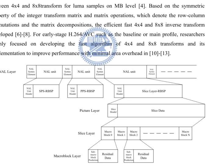
and ringing artifacts. However, for high-quality video, large block-size transform must be used not only to preserve fine details of the image but also to obtain the better energy compaction. High-definition (HD) applications adopt main profile, extended profile and high profile in H.264/AVC, and they require complicated design. Also, H.264/AVC offers various scalabilities to be adapted to the receipt condition of the data and the various multimedia applications [3]. Transform process of H.264 requires 8x8 transforms for high-definition applications, and 4x4 transforms for general applications. To meet scalabilities, transform module must process both 8x8 integer transform operations and 4x4 integer transform operations. Therefore, design of 8x8 transforms and 4x4 transforms into unified block is an important issue in H.264/AVC coder. High proﬁle in H.264/AVC Fidelity Range Extension (FRExt), which is a new amendment added in H.264 standard, includes 8x8 integer transform and allows the decoder to adaptively choose between 4x4 and 8x8transform for luma samples on MB level [4]. Based on the symmetric property of the integer transform matrix and matrix operations, which denote the row-column permutations and the matrix decompositions, the efficient fast 4x4 and 8x8 inverse transform developed [6]-[8]. For early-stage H.264/AVC such as the baseline or main proﬁle, researchers mainly focused on developing the fast algorithm of 4x4 and 8x8 transforms and its implementation to improve performance with minimal area overhead in [10]-[13].

NAL Layer SyntaxNAL

Element NAL unit NAL unit NAL

Syntax

Element NAL unit NAL Syntax Element NAL Unit Header SPS-RBSP NAL Unit Header PPS-RBSP NAL Unit

Header Slice Layer-RBSP Slice

Header Slice Data

Macro block 0 Macro block 1 Macro block 2 Macro block N Sub-macro block Prediction Residual Data Residual Data NAL Syntax Element Macroblock Layer Slice Layer Picture Layer Sub-macro block Prediction

(12)

3

In normal system architecture, the block of syntax parser employs in decoding the bit-stream on NAL layer, picture layer, and slice layer, given as Figure 2. Syntax element parser is also the top module to control all sub-system such as inverse integer transform, CABAD, VLD, intra-prediction, inter-intra-prediction, and so on.

1.1 Introduction of H.264/AVC decoding flow

In common with earlier coding standards, H.264 does not explicitly define a CODEC (encoder/decoder pair) but rather defines the syntax of an encoded video bitstream together with the method of decoding this bitstream. In practice, a compliant decoders are likely to include the functional elements shown in Figure 3.With the exception of the deblocking filter, most of the basic functional elements (prediction, inverse transform and inverse quantization) are present in previous standards (MPEG-1, MPEG-2, MPEG-4, H.261, H.263) but the important changes in H.264 occur in the details of each functional block.

Reference frame MC Intra prediction Current frame (reconstructed)

Filter IIT Q-1 Reorder Entropy_decode NAL

P Inter Intra INTER prediction Dn + + X Fn

Figure 3. Block diagram of H.264/AVC decoder

The decoder receives a compressed bitstream from the NAL and entropy decodes the data elements to produce a set of quantized coefficients X. These are scaled and inverse transformed to give Dn. Using the header information decoded from the bitstream, the decoder creates a

(13)

4

prediction block (PRED), identical to the original prediction formed in the encoder. PRED is added to Dn to produce Fn which is filtered to create each decoded block (Current frame).

(14)

5

1.2 Motivation & Design Challenges

The transform process that converts image or motion compensated residual data into another domain. H.264 supports several inverse integer transforms. Table 1 shows the motivation comparison with the previous standard. Our target is to reduce the complexity of inverse integer transform and make it fast. If we can reduce transform complexity, we can also reduce power consumption and hardware cost, moreover, increase the throughput. By applying the concept of hardware sharing, power-area requirement for the hardware implementation of the inverse integer transform will be reduced by sharing the hardware resources. Optimizing 4x4, 8x8 and Hadamard inverse transforms algorithm of the H.264/AVC decoder, we obtain low power consumption, high performance and small area design. To reduce power consumption and enhance performance of the transform with a minimum area overhead remain the design challenges in H.264/AVC video standard.

Table 1. Motivation comparison of standards

Feature/Standard MPEG-1 MPEG-2 MPEG-4 part 2 H.264/MPEG part 10

Macro block size 16x16

16x16 (frame mode)

16x8 (field mode) 16x16 16x16 Block size 8x8 8x8 16x16, 16x8, 8x8

16x16, 8x16, 16x8, 8x8,4x8, 8x4, 4x4

(15)

6

1.3 Thesis Organization

An introduction of H.264/AVC video coding standards are given in this section. The rest of this thesis is organized as follows. Chapter 2 describes the related works for inverse integer transforms, the overview of H.264/AVC profiles and previous works. In Chapter 3, we describe our proposed algorithm and hardware architecture for 4x4, Hadamard and 8x8 inverse integer transform. In this chapter, we also implement the hardware sharing algorithm & architecture, and take an in-depth discussion about Comparison and implementation of hardware sharing architecture. Moreover, we show 4 kinds of Inverse integer transform module design including hardware sharing and according to our proposed algorithm, system integration architecture and comparison of the proposed design with others shows in 0. Finally, we make the conclusion and future works in the last Chapter 5.

(16)

7

Chapter 2 Related Works

In this chapter, we will describe the overview of the H.264/AVC traditional inverse integer transform algorithm for 4x4, Hadamard and 8x8 MB.

2.1 Inverse Integer Transform Algorithm

2.1.1 Overview of the Inverse Integer Transforms

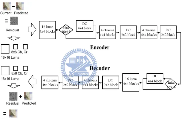
H.264/AVC uses a macroblock (MB) as a basic data unit. Our input includes coefficients and flags decoded by the entropy decoder (CAVLC or CABAC). It contains luma part and chroma part. The inter-prediction or intra prediction module finds a macroblock which is similar to current one from reference or present frames. However, the founded MB usually does not perfectively match with the current one, and the differences are called residuals (or prediction error) as shown in Figure 4. The residuals are inversely transformed which are then reordered and entropy encoded. At the decoder side, these entropy-encoded coefficients are decoded back to coefficients. After reordering, coefficients are inversely transformed to residuals data. Finally the residuals are combined with prediction data to reconstruct a MB.

(a.) Current Frame (b.) Predicted Frame (c.) Residuals

Figure 4. Residuals (prediction errors) between current and reconstructed frame

There are one 16x16 luma block and two 8x8 chroma blocks (Cb, Cr) within a macroblock. A 16x16 luma block can be divided into four 8x8 blocks, and each consists of four 4x4 blocks. A chroma 8x8 block contains four 4x4 blocks. In Figure 4, every 4x4 (or 2x2) block is numbered

(17)

8

according to decoding order. If a macroblock is coded by intra 16x16 prediction mode as shown in Figure 5(a), block -1 which contains DC coefficients of every 4x4 luma block will be processed first. The DC coefficients are filled back to upper-left corner of each 4x4 block in a16x16 luma block. Next, the luma residual blocks 0-15 are processed. After luma block is decoded, chroma DC blocks 16 and 17 are processed, and filled back to upper-left corner of each 4x4 block in an 8x8 chroma block. Finally, chroma residual blocks 18-25 are processed. If current macroblock type is non-intra 16x16, the processing order is the same except that it has no luma DC block as shown in Figure 5(b).

Cb Cr

Luma

(a) Intra 16x16 macroblock

Cb Cr

Luma

(18)

9

Figure 5. Scanning order of residual blocks within a macroblock

Three kinds of inverse integer transform are adopted depending on the type of residual blocks: 4x4 Hadamard transform for luma DC block (block -1), 2x2 Hadamard transform for chroma DC block (block16, 17), and 4x4 integer transform for all other types of 4x4 blocks (block 0-15, 18-25).Figure 6 shows the decoding flow diagram. We will emphasize on the decoder side. DC 4x4 block Intra 16x16 Current Predicted Residual 16x16 Luma 8x8 Cb, Cr Reconstructed 8x8 Cb, Cr 16x16 Luma Residual Predicted

Encoder

Decoder

Figure 6. H.264/AVC Encoding/Decoding flow diagram

If 4x4 inverse transform is employed, the luma part is divided into one luma DC 4x4 block and 16 luma AC 4x4 blocks. On the other hand, if 8x8 transform is applied, the luma part is divided into four 8x8 blocks. The chroma part is divided into two chroma DC 2x2 blocks and eight chroma AC 4x4 blocks in both cases.

(19)

10

In the following sub-sections, we will describe the traditional 4x4, Hadamard and 8x8 inverse integer transform algorithms.

(20)

11

2.1.2 Traditional 4x4 Inverse Integer Transform

In the H.264/AVC standard, the inverse integer transform operates on 4x4 blocks of residual data after motion-compensated prediction or intra prediction [4]. However, only two types of 4x4 inverse transforms are defined for the H.264/AVC decoder. The first type is the 4x4 inverse integer transform, which is defined as Eq. 2.1, where the 4x4 inverse integer transform coefficient matrix

A

_{4 i}defined as Eq. 2.2

4

(

)

4 4 4 T T i i i i i

X



A

Y E A





A FA

_{Eq. 2.1} 4 4

1

1 1/2

-1

1 -1/2 -1

1

1 -1

1 -1/2

T i i

A



























_, 2 2 2 2 2 2 2 2 i

a

ab a

ab

ab b

E

a

ab a

ab

ab b



























and

F Y E

 

_i Eq. 2.2

Then

A

_{4 i}and

E

_i are given by and where a=1/2 and b= 2 5. The “ ” means each element of Y is multiplied by the scaling factor in the same position in matrix

E

_i [3]. Since the scaling matrix

i

E

could be merged into the inverse quantization and pre-scaled process to reduce the number of multiplication process. Figure 7 show the traditional 4x4 inverse integer transform algorithm.

(21)

12

Figure 7.Traditional 4x4 inverse integer transform

2.1.3 Traditional Inverse Hadamard Integer Transform

The second type is the 4x4 inverse Hadamard transform (also known as the luma DC transform). The inverse Hadamard transform is defined as Eq. 2.3, where XD is the 4x4 DC component of a 16x16 intra mode macroblock.

T D 4i D 4i

W = H X H

Eq. 2.3

The 4x4 inverse Hadamard integer transform coefficient matrix H4i defined as Eq. 2.4

and Figure 8 shows the traditional two dimensional inverse Hadamard fast algorithm.

4i 1 1 1 1 1 1 -1 -1 H = 1 -1 -1 1 1 -1 1 -1             Eq. 2.4

(22)

13 T D 2i D 2i

X = H W H

, with 2i

1 1

H =

1 -1













Eq. 2.5

In the H.264/AVC standard, the 2x2 chroma DC transform is also defined. Since it is implied in the 4x4 inverse Hadamard transform.

Figure 8.Traditional 4x4 inverse Hadamard integer transform

2.1.4 Traditional 8x8 Inverse Integer Transform

The 8x8 forward and inverse integer transforms can be performed in a similar with 4x4 manner. 8x8 forward integer transform can be realized by the following equivalent form as Eq. 2.6, where

~ f

E is the scaling matrix. Meanwhile, 8x8 inverse integer transform is described as Eq. 2.7, where

E

~ iis the scaling matrix.





~ 8 8 T f f f

Y



C XC



E

Eq. 2.6

(23)

14

 

~ 8 8 8 8 T T i i i i i

X



C Y E C





C YC

Eq. 2.7

The

_C

_8i is the corresponding 8x8 inverse transform matrix and we note that ₈ ₈T

i f

C



C

. Coefficient of 8x8 inverse integer transform for high profile is shown in Eq. 2.8. The 8x8 transforms are only applied to luma blocks.

8

12

8

10

8

6

4

3

8

10

4

3

8

12

8

6

8

6

4

12

8

3

8

10

8

3

8

6

8

10

4

12

8

3

8

6

8

10

4

12

8

6

4

12

8

3

8

10

8

10

4

3

8

12

8

6

8

12

8

10

8

6

4

3

i







_















_

















_









_













C

Eq. 2.8

(24)

15

Figure 9. Traditional 8x8 inverse integer transform

In the previous section, we already know the H.264 integer inverse transform (4x4, Hadamard, 8x8) their principle and algorithms. For the implementation, the first one dimensional inverse integer transform block executes the transformation of row pixels and the second one dimensional inverse integer transform block performs the transformations of column pixels. Such as, Figure 9 is that the traditional 8x8 inverse integer transform method for implementation of hardware algorithm.

(25)

16

2.1.5 Traditional Hardware Sharing Design

Figure 10. Traditional hardware sharing design [19]

In order to reduce the gate count required for the two different transform processors, using multi transform (hardware sharing) algorithm that combine the three transform units into one multiple function transform processor which can execute all the three transform operations in H.264. In traditional hardware sharing architecture shown in Figure 10, the one dimensional transform can be any type of the transform. By the observation of Figure 7and Figure 8, we can find that every one-dimensional transform contains 8 arithmetical operations. In order to get a clear view of how to achieve hardware sharing transforms in a single design, we overlap Figure 7, Figure 8, and Figure 9 together. In Figure 10, all the adders have three inputs. It means that a

(26)

17

common input which is not changed by the transform type exists. Furthermore, Figure 10 is the fully extended of [19] into 64 pixels.

(27)

18

2.2 H.264 Profiles and Levels

H.264/AVC defines four profiles: baseline, extended, main and high profile. Baseline profile is usually used in low bit-rate applications. Extended profile, also called streaming profile, is designed for internet communication. Main profile is suitable for broadcast and storage applications. High profile, also called Fidelity Range Extension (FRExt), is intended for high resolution applications characterized by large block transform and large prediction blocks.

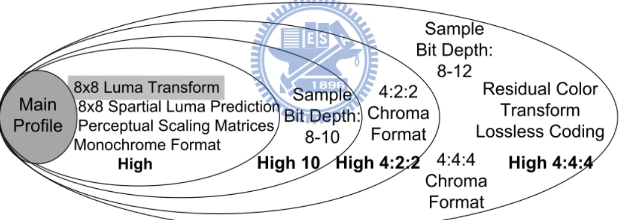
The high profile is further classified into four sub-profiles: High, High 10, High 4:2:2 and High 4:4:4, as depicted in Figure 11. These features include 8x8 luma transform, 8x8 spatial luma prediction, custom scaling matrix, deeper sample bits and lossless coding. Among them, the 8x8 luma transform is the key.

Main Profile

8x8 Luma Transform

8x8 Spartial Luma Prediction Perceptual Scaling Matrices Monochrome Format High Sample Bit Depth: 8-10 High 4:2:2 Sample Bit Depth: 8-12 4:2:2 Chroma Format High 10 4:4:4 Chroma Format Residual Color Transform Lossless Coding High 4:4:4

Figure 11. High profile classification and features

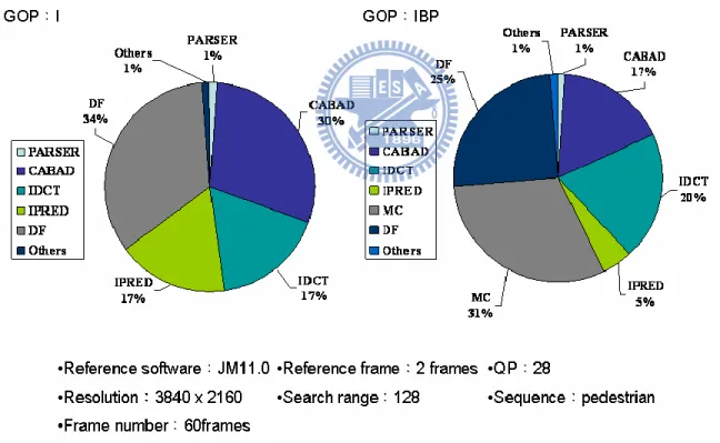
Figure 12shows the profiling result of decoding a high profile video sequence. The inverse integer transform consumes about 17% to 20% of CPU time. Therefore, we design a low power inverse integer transform for integration into H.264/AVC decoder depicted in Figure 1.

(28)

19

Some important H.264 profiles and their special features are:

Baseline Profile: Only I and P type slices are present, only frame mode (progressive) picture types are present, Only CAVLC is supported.

Main Profile: Only I, P, and B type slices are present, Frame and field picture modes (in progressive and interlaced, modes) picture types are present, Both CAVLC and CABAC are supported, ASO is not supported, FMO is not supported.

High Profile: Only I, P, and B type slices are present, Frame and field picture modes (in progressive and interlaced modes) picture types are present, Both CAVLC and CABAC are supported, ASO is not supported, FMO is not supported, 8x8 transform supported, Scaling matrices supported.

Figure 12.H.264 decoder profiling results

All of these profiles also support mono chroma coded video sequences, in addition to typical 4:2:0 video. The difference in capability among these profiles is primarily in terms of supported sample bit depths and chroma formats. However, the high 4:4:4 profile additionally supports the

(29)

20

residual color transform and predictive lossless coding features are not found in any other profiles. The detailed capabilities of these profiles are show in Table 2.

Table 2.Coding tools in different profiles of H.264/AVC standard

Coding Tools Baseline Main Extend High High 10 _4:2:2High _4:4:4High

4:2:0 Chroma formats Yes Yes Yes Yes Yes Yes Yes Monochrome video format (4:0:0) No No No Yes Yes Yes Yes 4:2:2 Chroma Format No No No No No Yes Yes 4:4:4 Chroma Format No No No No No No Yes 8 Bit Sample Bit Depth Yes Yes Yes Yes Yes Yes Yes 9 and 10 Bit Sample Depth No No No No Yes Yes Yes 11 to 12 Bit Sample Depth No No No No No No Yes 8x8 vs. 4x4 transform adaptivity No No No Yes Yes Yes Yes Quantization scaling matrices No No No Yes Yes Yes Yes Separate Cb and Cr QP control No No No Yes Yes Yes Yes

Residual Color Transform No No No No No No Yes Predictive Lossless Coding No No No No No No Yes Flexible Macroblock Ordering (FMO) Yes Yes No No No No No

(30)

21

2.3 Previous Works

In recent years, many researchers proposed a number of optimized algorithms to compute the transforms used in H.264/AVC. The major focus of the research has been to develop fast algorithms for the transform unit.

2.3.1 Parallel 4x4 transform and inverse transform

Architecture for MPEG-4 AVC/H.264 [5]

The multi-transform approach is good for low power and saving the hardware area. Chen’s design [5] is the first multi-transform architecture. They proposed a low power multi-transform architecture. They analyze residuals characteristics and propose a switching power suppression technique for saving data transition power. The design outputs four values every cycle. Their design achieves throughput of eight pixels per cycle and consumes 14.40mW at 200MHz.

Figure 13. (Re-designed) parallel transform architecture

This architecture is very compact for the 4x4 inverse transform, the gate count is only 4983. The processing speed can be achieved to 1Gpixels/sec at 200MHz. It is sufficient for the existing video formats including HDTV formats. But this architecture is very limited because it can only support 4x4 block. Moreover, if we want to use this architecture and extend to 8x8, it will have almost 4 times overhead. Therefore, this will cost large power consumption and hardware cost. This design still exists some way to accelerate the processing speed and reduce the hardware cost.

(31)

22

2.3.2 Low Cost Hardware sharing Architecture of Fast

Inverse Transforms for H.264/AVC and AVS

Applications [8]

The 1-D fast algorithms and their hardware sharing design for the 1-D inverse transforms of H.264/AVC and AVS are proposed by using the symmetric property of the integer DCT matrix and the matrix decompositions. In this paper hardware-sharing architecture for H.264/AVC and AVS is realized by the offset computations and the pipelined design. Thus, the hardware cost of the proposed sharing architecture for H.264/AVC and AVS is smaller than that of the individual and separate realizations. This design implemented by pipeline stage to increase the performance of inverse transform.

Figure 14. Block diagram of the proposed hardware sharing architecture of fast 2x2, 4x4 and 8x8 inverse transforms for H.264/AVC and AVS with four pipeline phases [8]

In this paper, the 1-D transform is further divided into two smaller matrix-vector operations by even-symmetric or odd-symmetric. Therefore, its size is smaller. But the latency is increased

(32)

23

to 22 cycles because it only consumes one coefficient every cycle. Then the power consumptions of the 8x8 inverse integer at H.264/AVC mode and the 8x8 inverse at AVS mode at 62.5 MHz are 34.266mW and 37.785mW, respectively. Because of the supporting two video standards, need to add extra adding offset computations that use extra registers to completely satisfy two video standards. Therefore the area overhead and power consumption still need to be improved. This design still exists some way to reduce the hardware cost and power consumption.

2.3.3 A High Performance Inverse integer Transform

Architecture for the H.264/AVC Decoder[12]

In this paper, a high-performance inverse transform architecture for the H.264/AVC decoder is proposed. The proposed architecture utilizes the block multiplication and permutation matrices. This architecture uses the matrix decomposition method to reduce the complexity of 4x4 inverse transform. By applying permutation matrices, the inverse transform matrix is regularized and the inverse Hadamard transform is merged into inverse transform with a minor modification.

(33)

24

This design has higher throughput for computing inverse transform and inverse Hadamard transform. It has also higher hardware efficiency through the measure of DTUA for computing inverse transform and inverse Hadamard transform. In hardware architecture in each block A2,

B2, C2, D2, they use traditional 4x4 inverse transform algorithm for implementation and too

much extra logic was required to completely satisfy H.264/AVC standard. Therefore area and power consumption still need to be improved.

2.3.4 Configurable, Low-power Design for Inverse Integer

Transform in H.264/AVC[16]

This paper presented a configurable, low-power design for the inverse integer transform in H.264/AVC. The power consumption is drastically reduced by employing an input block-type aware algorithm with variable number of operations for the computation of the inverse integer transform. This algorithm takes advantage of significant number of zero-valued transformed coefficients in a typical input block. Additionally, the area overhead was reduced by designing basic configurable processing blocks in order to share the hardware resources (adders) for different input block types.

(34)

25

The internal organization of this block is depicted in Figure 16. Since the processing block M1-M3 are derived from M4 (Figure 17) and have the similar structure, therefore, we can design a configurable processing units (CM14, CM24, and CM34) with overlapped functionality to reduce the hardware resource requirement for its implementation.

The configurable processing units (CM14, CM24, and CM34) as the name suggest can be configured to provide processing for either (M1, M4), (M2, M4), or (M3, M4) using the appropriate control signal.

Figure 17. Data flow diagram for (a) M1, (b) M2, (c) M3, and (d) M4 cases.

The internal architecture for these configurable units is depicted in Figure 18(a)-(c). Therefore, no additional (34) adders are required anymore because of configurable processing units. Furthermore, the input registers (in CM24) are also shared among processing for data vectors.

(35)

26

Figure 18. Data flow diagram for (a) CM14, (b) CM24 and (c) CM34.

The new algorithm is derived from the fast one dimensional inverse integer transform. This paper focuses on the low power design that consumes significantly less dynamic power (up to 80% reduction) when compared with existing conventional design for the inverse integer transform. In some blocks, they use traditional 4x4 inverse transform algorithm and this architecture processing speed is very slow that can’t achieve the high resolution such as full HD in H.264/AVC.

2.3.5 A Reconfigurable IDCT Architecture for Universal

Video Decoders[17]

The reconfigurable architecture has become more and more popular. It not only decreases the time of research and development but also saves fabrication cost. Moreover, the proposed reconfigurable inverse integer transform architecture can support 3 different video standards such as VC-1, MPEG and H.264/AVC. The block diagram is shown in Figure 19.

(36)

27

Figure 19. Block diagram of reconfigurable inverse integer transform

Figure 20. Architecture of reconfigurable one dimensional inverse integer transform

a) b)

(37)

28

They propose the reconfigurable one dimensional inverse integer transform architecture combined from two modes in Figure 20 in order to meet the requirements of various video standards. Adder kernel unit, we can find that any combinations of the input signals are composed of {00~11} or {0000~1111}. Therefore the computational results in every row can be generated by adder kernel even and odd part in figure 21. We can simplify the adder kernel into thirteen adders only: two adders in the even parts, figure 21a, and eleven adders in the odd part, figure 21b. Routing network is for VC-1 inverse integer transform. Stage 3 is the shifter and adder tree unit, using two’s complement concept to implement the total sums. Stage 4 is the post-adders.Reconfigurable inverse integer transform architecture is implemented for universal video decoders. It is the key point of this paper to reinforce the high throughput and to reduce power consumption and improve the throughout utilizing parallelism. This architecture can support 3 different video standards. The power consumption is 3.4mW at 100MHz, hardware cost is 11.6k and the throughput rate is 800Mpixels/sec. but throughput is still lower than the state of the art such as [7], [10], [12]. In this paper, what kind of fast algorithm that used is not clear and in order to achieve different video standards that use too much extra registers therefore hardware cost still need to be improved.

(38)

29

2.4 Summary

Table 3 summarized the above approaches. Each has distinct strength and weakness. We take 4x4 transform supporting, 8x8 transform supporting, Hadamard transform supporting, power consumption, hardware cost, DTUA, and throughput as our comparison items.

Table 3. Supporting features comparison Hwangbo Su [8] Liu [9] Chen [10] Cheng [11] Su [13] Shia [14] Lin [15] Lai [17] [7] [12] 4x4 transform Y Y Y Y Y Y N Y Y Y 8x8 transform Y N Y N N N Y Y Y N Hadamard Y Y Y N Y Y N N N Y low power N N N N Y N N N N Y low area N N Y Y N N Y Y Y N High DTUA N Y N N N N N N N N High Throughput Y Y N N N Y N N N N

We also take an effort to evaluate several previous works and classify into three strategies: Low power aware, low hardware cost aware and high throughput aware. In Figure 22, we classify previous works as their strategy. Each strategy represents the major improvement in conventional inverse integer transform decoder. Each strategy represents the major improvement in conventional inverse integer transform decoder.

(39)

30

(40)

31

Chapter 3 Proposed Algorithm & Architecture

In this chapter, we propose our 4x4, Hadamard and 8x8 inverse integer transform fast one dimensional butterfly algorithms, pipeline hardware architectures and in Section 3.4 proposed their hardware-sharing design for 4x4, Hadamard and 8x8 inverse integer transforms of H.264 video decoder. In our algorithms we use matrix decomposition method to reduce the complexity of inverse integer transforms to reduce the power consumption, hardware cost and raise the throughput and hardware efficiency in H.264/AVC. Matrix decomposition utilizes the permutation matrices. All Inverse integer transforms Hardware architecture designs are implemented with pipelined architecture. Thus, our design’s power consumption and hardware cost are smaller when comparing to previous works.

The area overhead for the inverse integer transforms unit can be reduced by sharing the hardware resources between the independent processing units by designing the new fast butterfly algorithm. In next sub-sections, we will discuss more details about new fast 4x4, Hadamard, 8x8 butterfly algorithms.

3.1 Fast 4x4 Inverse Integer Transform

3.1.1 Fast 4x4 Inverse Integer Transform Algorithm

Fast 4x4 inverse integer transform algorithm is proposed in this part. First we will derive the formulas then algorithms which will be implemented in hardware design. We know that from the previous chapter 4x4 inverse integer transform coefficient matrix (Eq. 3.1) is follows,

4

1

1 1/2

-1

1 -1/2 -1

1

1 -1

1 -1/2

i

A



























Eq. 3.1

(41)

32

We will use the matrix decomposition method to reduce the complexity of inverse integer transform which also means reduce the power consumption, hardware cost in terms of gate count. Therefore we define two permutation matrices Tc and Tr as described below,

1 0 0 0

0 1 0 0

=

0 0 0 1

0 0 1 0

c

T

























r

T

   







_{   }









   







_{   }







Eq. 3.2 And where 4 4

( )

T

( )

T

, ( )

T

( )

T c c c c r r r r

T T



T T



I T T



T T



I

Eq. 3.3

I4 is an identity matrix of order 4. By using these permutation matrices then we will get a

new matrix ~ 4i

A

, where the ~ 4i

A

matrix is described as follows,

~ 4i

( ) ( )

c 4i r

A



T A T

1

1 1 2

1

1 1 2

1

1 1 2

   



 





_{   }

 

_

 

_{   }





 







   

 



 

   





_{   }

 

_

 

_{   }





 



1 1

1 1/ 2

1 1 1/ 2

1 1 1

1 1/ 2

1

1 1/ 2

1 





_

















_{ }







Eq. 3.4 We can re-write the inverse integer transform coefficient matrix from Eq.3.4 matrix multiplication,

(42)

33 ~ 4

( )

4

( )

T T i c i r

A



T

A T

Eq. 3.5

Then if we can use

_A

~_4imatrix to represent with 2x2 matrix form (Eq. 3.6)

~ 2 4 2

1 1

1 1/ 2

1

1 1/ 2

1 =

1 1

1 1/ 2

1

1 1/ 2

1

i

A











_





_



_

_











_{  }

_



_

_{ }

_

_



_

_

_



_

_{ }

_









 









H

Q

H

Q

Eq. 3.6

Where

H

₂ and

Q

are

1 1

1

1 



 

_







2

Η

1 1/ 2

1/ 2

1 



 

_







Q

Eq. 3.7

Then we use the matrix operation rule to derive one of the following equations (Eq. 3.8);











_

_

_









2 2

A B

H

I

A B

A -B

Where 2

1 0

0 1





 







I

Eq. 3.8

And where _{denotes the Kronecker product, matrix operation as follows (Eq. 3.9). Assume}

that the dimension of the matrix A is NxP, B is MxQ,

PQ MN NP N N P P

a



















B

A







2 1 2 22 21 1 12 11 Eq. 3.9

Another means the direct sum operation which matrix operation express as follows (Eq. 3.10),

N N 2 2

0



















B

A

B

A

Eq. 3.10

(43)

34

If we apply Eq. 3.8 matrix operation rule to Eq. 3.5 then we can re-derive 4x4 inverse integer transform coefficient matrix,

A

_4ire-expressed as follows,









~ 4

( )

4

( )

2 T T T T i c i r c r

A



T

A T



T H

₂



I

₂

H

₂



Q T

Eq. 3.11

3.1.2 Fast 4x4 Inverse Integer Transform Architecture

According to Eq. 3.11, the first stage of the hardware design

T

_rT and the last stage

T

_cT permutations are just wire connection which represents no arithmetic computation. We use 2 pipeline stages to finish the operation. Figure 23 shows pipeline hardware architecture to represent the 4x4 inverse integer transform and we use the pipeline stages to help us simplify the design and speed up the hardware to achieve the higher resolution such as HD 1080, QFHD(4*HD 1080) @ 30fps.

(44)

35

In pipeline hardware architecture we use fast butterfly algorithm data flow like Figure 24 to implement 4x4 inverse integer transform. The complexity of this proposed fast 4x4 inverse integer transform needs2 shift operations and 8 additions.

Figure 24. New fast algorithm of 4x4 inverse integer transform.

3.2 Fast Inverse Hadamard Integer Transform

3.2.1 Inverse Hadamard Integer Transform Algorithm

The Hadamard inverse integer transform is given by;

T

D 4i D 4i

W = H X H

Eq. 3.12 We know that from the previous chapter Hadamard inverse integer transform coefficient matrix, H4i as follows, 4i

1 1

1

1 1 1 -1 -1

H =

1 -1 -1 1

1 -1 1 -1

























Eq. 3.13

The Hadamard inverse integer transform can be performed in a similar manner. For the Hadamard inverse integer transform, we use the same permutation matrices,

T

_r and

T

_c ,

(45)

36 T T c r

T





T



_

_





2 2 4i 2 2

H

-H

Eq. 3.14

(

2 2

)(

2 2

)

T T c r



T H



I

H



H T

Eq. 3.15 WhereH2 is the same matrix given in (Eq. 3.7) before. The first stage of the Hadamard

inverse integer transform hardware design T r

T

and the last stage T c

T

permutations are just wire connection which represents no arithmetic computation.

3.2.2 Inverse Hadamard Integer Transform Hardware

Architecture

Figure 25 shows 2 pipeline hardware architectures to represent the 4x4 Hadamard inverse integer transform that we use the pipeline stages to help us simplify the design and speed up the hardware.

T

r

T

4x4 Input 4x4 Output

_T

c

T

means pipelined register array

pipelined stage 1 pipelined stage 2

()



22

HH

()



22

HI

(46)

37

Figure 26 shows 4x4 Hadamard inverse integer transform implemented by using new fast butterfly algorithm data flow. The complexity of this proposed fast 4x4 Hadamard inverse integer transform needs just 8 additions without any shift operation.

(47)

38

3.3 Fast 8x8 Inverse Integer Transform

3.3.1 Fast 8x8 Inverse Integer Transform Algorithm

As we know from the previous chapter 8x8 transform coefficient matrix as follows,

8

12

8

10

8

6

4

3

8

10

4

3

8

12

8

6

8

6

4

12

8

3

8

10

8

3

8

6

8

10

4

12 / 8

8

3

8

6

8

10

4

12

8

6

4

12

8

3

8

10

8

10

4

3

8

12

8

6

8

12

8

10

8

6

4

3

i







_















_

















_









_













C

Eq. 3.16

According to the fast computations in [2], the fast 8x8 inverse integer transform that we use further matrix decomposition into 3 stage matrix multiplication as below,

1 2 3 8i 8i

. .

8i 8i

C



C C C

Eq. 3.17

These 3 matrices

C

_8i1

C

_8i2,

C

_8i3 are,

1 8

1 0 0 0

1

0

0 0 1 0 0

0

1

0

0 0 0 1 0

0

1

0 0 0 0 1

0

1 0 0 0 1

0

1 0 0 1 0

0

1

0 0 1 0 0

0

1

0

0 1 0 0 0

1

0

i





























_















_

















C

Eq. 3.18

(48)

39 2 8

1 0

1

0

1 0 1

0

1

0

0 0 1

0 1 0

0

0 1 0

1

0

1

0

3 0 0

0

1

0

2

3 0 1

0

1

0

1

2

3 0 0

1

0

1

0

1

2

3 0 0

0

1

2

i





















_















 





_













_





















C

Eq. 3.19 3 8

1

0

1

0

1

0

1

0

1

0

1

0

2

1

0

1

0

2

1

0

1

0

4

1

0

1

0

4

1

0

1

0

4

1

0

1

4

i







_





















_











 



































_











C

Eq. 3.20

Eq. 3.18,

C

_8i1 can be further decomposed into,





1 8i



.

2



~ T c 4

C

T

H

I

Eq. 3.21

(49)

40

Where

I

₄identity matrix with order 4 and permutation matrix

~ c

T

is defined by;















1

0

1

0

1

0

1

4

I

Eq. 3.22 ~

1 0 0 0 0 0 0 0

0 1 0 0 0 0 0 0

0 0 1 0 0 0 0 0

0 0 0 1 0 0 0 0

0 0 0 0 0 0 0 1

0 0 0 0 0 0 1 0

0 0 0 0 0 1 0 0

0 0 0 0 1 0 0 0

c

























 



























T

Eq. 3.23 Eq. 3.19, 2 8i

C

can be further decomposed into,

~ 2 8i

[(

2 2

)(

2 2

)]

1 T









C

I

H

I

Q

Eq. 3.24

Where

I

₂identity matrix with order 2 and permutation matrix

~ 2

I

and

Q

1is equal to as below;

2

1 0

0 1

I

 





_





_, ~ 2

0 1

1 0

I

 





_





1

3

1

0

2

3

1

0

1

2

3

1

0

1

2

3

0

1

2 













_







 





_





















Q

Eq. 3.25

(50)

41

In Eq. 3.25, 3x/2 can be decomposed to x+(x>>1). (x>>1) means 1 bit right shift. Eq. 3.20,

C

_8i3 can be further decomposed into,

~ ~ 3 3 8 8 T i



i



r

C

C T

Eq. 3.26 Where ~ r

T

is, ~ 1 0 0 0 0 0 0 0 0 0 0 0 1 0 0 0 0 0 1 0 0 0 0 0 0 0 0 0 0 1 0 0 0 1 0 0 0 0 0 0 0 0 0 0 0 0 1 0 0 0 0 1 0 0 0 0 0 0 0 0 0 0 0 1 r                            T Eq. 3.27 And where ~ 3 8i

C

can be further decomposed into,

3

8

(

2 2

)

3

T

i





C

~

H

Q

Eq. 3.28

Where in (Eq. 3.28) Q2 and Q3, defined as,

2

1

1 2 and

1

2 







 





_











Q

3

1

0

4

1

0

1

0

4

1

0

1

0

4

1

0

1

4 



















 





_





















Q

Eq. 3.29

(51)

42 ~ 3 8

[(

2

)

3

]

T T i





2





r

C

H

Q

Q T

Eq. 3.30

Similarly, in Eq. 3.29, x/2 and x/4 can be replaced by 1 bit right shifter (x>>1) and 2 bit right shifter (x>>2) respectively.

Then we can rewrite the 8x8 inverse integer transform matrix,

C

_8i can become as follows;

1 2 3 8 8 8 8 ~ _~ ~ 2 4 2 2 2 2 1 2 2 3

(

) {[(

)(

)]

} [(

)

]

i i i i T T T T c r

























C

C C C

T

H

I

H

I

Q

H

Q

Q T

Eq. 3.31

3.3.2 Fast 8x8 Inverse Integer Transform Hardware

Architecture

Same as 4x4 inverse integer transform, the first stage of the 8x8 inverse integer transform hardware design

T

_rTpermutation and the last stage

T

_cT that need no arithmetic computation to be implemented by hard-wire connection. We use 4 pipeline stages to implement the 8x8 inverse integer transform operation. Figure 27 shows pipeline hardware architecture to represent the 8x8 inverse integer transform. We use the pipeline stages to simplify the design and speed up the hardware to achieve the higher resolution such as HD 1080, QFHD (4*HD 1080) @ 30fps.

(52)

43 ~ T r

T

1 T

Q

3 T Q 8x 8 Output 8x8 Input

means pipelined register array Pipelined stage 1 Pipelined stage 2 Pipelined stage 3 Pipelined stage 4 ~ T c

T

Figure 27. Pipeline hardware architecture for fast 8x8 inverse integer transform.

x0 x1 x2 x3 x4 x5 x6 x7 -1 1/2 1/2 -1 -1/4 1/4 1/4 1/4 12 2 1 2 1 2 1 -1 -1 -1 -1 -1 -1 -1 -1 -1 -1 -1 -1 y0 y1 y2 y3 y4 y5 y6 y7 -1

(53)

44

Figure 28 shows 8x8 inverse integer transform by using new fast butterfly algorithm data flow. Total complexities of proposed fast 8x8 inverse integer transform are just 10 shift and 32 addition operations. In the next section, we will discuss about hardware sharing architecture of inverse integer transform for H.264/AVC decoder.

(54)

45

3.4 Hardware Sharing Algorithm & Architecture

First of all, we make all these 4x4 inverse integer transform, Hadamard inverse transform and 8x8 inverse integer transform into one group. It can be found that the inverse transform process is slightly similar. In order to achieve low power and hardware saving for the inverse integer transform unit, sharing the hardware resources between the independent processing units is investigated. For the Hardware sharing design, we have listed all inverse integer transform equations from (Eq. 3.11), (Eq. 3.15), (Eq. 3.31) as follows,









4 T T i



c 2



2 2



r

A

T H

I

H

Q T

4

(

2 2

)(

2 2

)

T T i



c





r

H

T H

I

H

H T

~ _~ ~ 8

(

2 4

) {[(

2 2

)(

2 2

)]

1

} [(

2 2

)

3

]

T T T T i



c



















r

C

T

H

I

I H

I

Q

H

Q

Q T

From the above three equations, it can be found that in all these operations have



_H

₂

_

_I

₂



same blocks. In this block, we will be able to do hardware sharing. Other 3 blocks which are

2



2

H

Q

,

H

2



H

2 and

H

2



Q

2 need to be operated in one hardware block. Since

Q

2is

the main hardware block, for Hadamard we need to use shift in the input circuit (scaling) will meet the

H

₂which is defined in Eq.3.7 in order to save the hardware cost, for 4x4 inverse integer transform that doesn’t need any scaling in the input circuit because of

Q

₂=

Q

_{in (Eq.} 3.29) and (Eq.3.7). Figure 29 shows the hardware sharing architecture for the fast 4x4, Hadamard, 8x8 inverse integer transforms. The hardware sharing part of the fast inverse integer transforms is (H₂I₂)(H₂Q in Figure 29. ₂)

應用於H.264/AVC視訊解碼器之低功耗反整數轉換

National Chiao Tung University

Department of Electronics Engineering

Master Thesis

Design of A Low Power Inverse Integer Transform for H.264/AVC

Decoding Applications

Student : Hüseyin Demirkaya

Advisor : Prof. Chen-Yi Lee

Design of A Low Power Inverse Integer Transform for

H.264/AVC Decoding Applications

研 究 生：王英杰 Student：Hüseyin Demirkaya

指導教授：李鎮宜 Advisor：Prof. Chen-Yi Lee

國 立 交 通 大 學

電子工程學系 電子研究所 碩士班

碩 士 論 文

Design of A Low Power Inverse Integer

Transform for H.264/AVC Decoding Applications

Student：Hüseyin Demirkaya

Advisor：Prof. Chen-Yi Lee

Department of Electronics Engineering

National Chiao Tung University

ABSTRACT

Acknowledgements

Contents

Figure Index

Table Index

Chapter 1

Introduction

1.1 Introduction of H.264/AVC decoding flow

1.2 Motivation & Design Challenges

1.3 Thesis Organization

Chapter 2

Related Works

2.1

Inverse Integer Transform Algorithm

2.1.1 Overview of the Inverse Integer Transforms

Encoder

Decoder

2.1.2 Traditional 4x4 Inverse Integer Transform

A

(

)

X



A

Y E A





A FA

1

1

1

1/2

1 1/2

-1

-1

1 -1/2 -1

1

1

-1

1 -1/2

A

A





























a

ab a

ab

研究生：王英杰 Student：Hüseyin Demirkaya

國立交通大學

電子工程學系電子研究所碩士班

碩士論文

_C