應用於彩色影像切割之區域性可靠資訊匯集

全文

(1)國立交通大學. 電子工程學系. 電子研究所碩士班. 碩士論文. 應用於彩色影像切割之區域性可靠資訊匯集 Local Belief Aggregation for Color Image Segmentation. 研究生: 詹景竹指導教授: 張添烜中華民國九十七年九月.

(2)

(3) 應用於彩色影像切割之區域性可靠資訊匯集 Local Belief Aggregation for Color Image Segmentation. 研究生: 詹景竹指導教授: 張添烜. Student: Jing-Chu Chan Advisor: Tian-Sheuan Chang. 博士. 國立交通大學電子工程學系電子研究所碩士班碩士論文. A Thesis Submitted to Department of Electronics Engineering & Institute of Electronics College of Electrical and Computer Engineering National Chiao Tung University in Partial Fulfillment of the Requirements for the Degree of Master In Electronics Engineering September 2008 Hsinchu, Taiwan, Republic of China. 中華民國. 九十七年. 九月.

(4)

(5) 應用於彩色影像切割之區域性可靠資訊匯集. 研究生: 詹景竹. 指導教授: 張添烜博士. 國立交通大學電子工程學系電子研究所碩士班. 摘. 要. 在彩色影像切割裡，馬可夫隨機場理論被用來解決如何給予畫面像素適當標籤的問題。在此論文裡，我們以區域的內部特性以及區域和區域之間的相關性來建立起馬可夫模型。然而，龐大的切割標籤數量，對於使用信任傳遞 (Belief Propagation, BP) 演算法來近似以馬可夫隨機場理論為基礎的彩色影像切割法遇到一些困難。這些困難包含了以下兩點：計算複雜度過高以及記憶體儲存空間過大而不敷使用的問題。在此論文裡，我們另外提出了一個利用地域性可靠資訊匯集的演算法來解決這些問題。這個方法主要是以限制鄰近點傳送進來的訊息數量為概念來達成目的。我們將此演算法套用到我們提出來的馬可夫模型上，利用近似的方式找出最大事後機率 (maximum a posteriori, MAP) 的結果。跟原本的信任傳遞演算法比較起來，我們提出的演算法可以減少相當多的記憶體儲存空間。在評量影像切割的結果方面，我們選擇與眾所皆知的平均位移 (Mean Shift) 演算法來做比較。在此，我們使用非監督方式的評比方法。這個方法主要是利用色彩視覺差異的特性設計而成的。實驗數據顯示，所提出的彩色影像切割演算法無論在主觀或是客觀的評比上，皆可以得到與平均位移演算法有相似的效果。除此之外，所提出的演算法在運算方面也比平均位移演算法還來的更具平行性。. i.

(6) ii.

(7) Local Belief Aggregation for Color Image Segmentation. Student: Jing-Chu Chan. Advisor: Tian-Sheuan Chang. Department of Electronics Engineering & Institute of Electronics National Chiao Tung University. Abstract. Markov Random Field (MRF) is used to solve the problem of labeling pixels in image segmentation. In this thesis, we formulate the MRF model based on the intra and inter region criteria. However, the enormous number of segment label in color image segmentation causes MRF-based color segmentation algorithm using belief propagation (BP) to suffer from complexity and storage explosion. To cope with this problem, this thesis also proposed a local belief aggregation (LBA) algorithm which restricts the number of messages to be aggregated from a neighboring node, to find the segmentation image that approximate the MAP solution of our MRF model. With the proposed LBA, memory storage is much reduced compared with the original BP algorithm. To evaluate the segmentation results, we compare the segmentation image with the well-known mean shift algorithm. Here, the unsupervised evaluation scheme using visible color difference is used as our objective evaluation metric. Experimental results show that the proposed color image segmentation algorithm can achieve a comparable result to mean shift algorithm both objectively and subjectively. Besides, the computation of LBA possesses more parallelism than the mean shift algorithm.. iii.

(8) iv.

(9) 誌. 謝. 首先，要感謝我的指導教授—張添烜博士，這兩年來給我的支持和鼓勵，引領我以正確的態度來面對與解決問題。在研究上，總是讓我能自由的發揮，並在遇到瓶頸的時候給予建議與協助。此外感謝老師提供豐富的實驗室資源，使我不但能充分的利用軟硬體設備來進行研究，也能有機會出國參與研討會拓展視野。因此，我對與老師的感激之情溢於言表。謝謝我的口試委員們，交大電子王聖智教授和清大電機陳永昌教授，感謝你們百忙中抽空來指導我，因為你們寶貴的意見讓我的論文更加完備。感謝 VSP 實驗室的好伙伴們，特別要謝謝引我入門的張彥中學長，帶領我從零開始，一點一滴的從研究中學習與成長，尤其是當我對困難感到迷惘時，總是不厭其煩的和我討論，並且提供我許多寶貴的意見與想法。感謝林佑昆學長、李國龍學長，你們對於經驗與知識的分享，讓我受用無窮。謝謝李得瑋學長、郭子筠學長和廖英澤學長耐心的教導我許多硬體設計的觀念與技巧，也感謝林嘉俊學長與吳秈璟學長，你們在研究上認真負責的態度是我學習的榜樣。感謝曾宇晟和蔡宗憲同學不時的給予研究上的幫忙與協助，能跟你們一起討論是一段很難得的過程。感謝張瑋城與戴瑋呈同學，和你們一起待在實驗室熬夜趕作業是一段很有趣的回憶。感謝黃筱珊學妹、陳之悠、沈孟維、許博淵、蔡政君與廖元歆學弟們，有你們的陪伴，我的碩士班生涯充滿了歡笑。謝謝實驗室的所有成員們，和你們一起努力的日子，都是我在交大寶貴的回憶。謝謝李韋磬同學，和你討論課業外的事情讓我的生活增添一些有趣的變化。感謝陳斯寗同學，謝謝妳的熱心相助，尤其是在最後的階段還抽空協助我檢查英文文法以及多次的聽我練習口頭報告並給我許多的建議。有妳這樣的朋友真是我的榮幸。最後要感謝默默支持我的家人們，我的爸媽與姊姊，你們的溫暖是我努力最大的支柱。在此，把本論文獻給所有愛我與所有我愛的人。. v.

(10) vi.

(11) Contents Chapter 1. 1.1. 1.2. 1.3.. Introduction .......................................................................................... 1 Background .................................................................................... 1 Motivation and Contribution.......................................................... 2 Thesis Organization ....................................................................... 3. Chapter 2. Previous Work ...................................................................................... 5 2.1. Mean Shift Algorithm .................................................................... 5 2.2. Watershed Algorithm ..................................................................... 9 2.2.1. Immersion-based Method ............................................................ 10 2.2.2. Toboggan-based Method .............................................................. 12 2.3. Markov Random Field based Algorithm...................................... 14 2.3.1. Markov Random Field Theory ..................................................... 14 2.3.1.1. Random Fields ............................................................. 15 2.3.1.2. Markov Random Fields................................................ 16 2.3.1.3. Gibbs Random Fields................................................... 18 2.3.1.4. Relation between MRF and GRF ................................. 19 2.3.1.5. MAP-MRF Framework................................................ 20 2.3.2. Application in Segmentation........................................................ 21 2.3.2.1. Deng’s Work ................................................................ 22 2.3.3. Inference Algorithm Using Loopy Belief Propagation ................ 23 Chapter 3. Color Image Segmentation Algorithm Using MRF Model............. 27 3.1. Algorithm Overview .................................................................... 27 3.2. CIE L*a*b* Color Space ............................................................. 29 3.2.1. Introduction .................................................................................. 29 3.2.2. Color Transform from RGB to CIE L*a*b* ................................ 30 3.2.3. Color Difference .......................................................................... 31 3.3. MRF Model Formulation ............................................................. 31 3.3.1. Likelihood and Prior .................................................................... 31 3.3.2. Model Approximation .................................................................. 32 3.4. Local Belief Aggregation ............................................................. 37 3.4.1. Reliable Message Aggregation .................................................... 37 3.4.1.1. Four-window Based Local Search Window................. 38 3.4.1.2. One-window Based Local Search Window ................. 40 3.4.2. Maximum Belief Segment State Selection .................................. 41 3.4.3. Region Merge Process ................................................................. 43 3.4.4. Convergence of Local Belief Aggregation................................... 45 vii.

(12) 3.5. 3.6.. MRF Model Comparison ............................................................. 46 Complexity Analysis and Comparison......................................... 48. Chapter 4. Experimental Results and Analysis .................................................. 51 4.1. Introduction .................................................................................. 51 4.2. Segmentation Results ................................................................... 52 4.2.1. Chen’s Quantitative Evaluation Metrics ...................................... 52 4.2.2. Comparison between One-window Based LBA and Four-window Based LBA ................................................................................... 54 4.2.3. Comparison between Different Segmentation Algorithms .......... 58 Chapter 5. 5.1. 5.2.. Conclusion and Future Works .......................................................... 63 Conclusion ................................................................................... 63 Future work .................................................................................. 63. Reference Appendix. ............................................................................................................. 65 ............................................................................................................. 69. viii.

(13) List of Figures. Fig. 2.1. Flow of the mean shift filtering. ................................................................................................. 6 Fig. 2.2. Example of mode seeking procedure and density estimation. .................................................... 7 Fig. 2.3. Flow of the mean shift segmentation. ........................................................................................ 8 Fig. 2.4. Visualization of mean shift filtering and segmentation results for gray level data [6]. (a) Input image. (b) Mean shift mode seeking paths. (c) Mean shift filtering result. (d) Mean shift segmentation result. ................................................................................................................. 9 Fig. 2.5. Example of one dimensional signal using immersion-based watershed approach. .................. 10 Fig. 2.6. Example of one dimensional signal using toboggan-based watershed approach. .................... 12 Fig. 2.7. Flow chart of the Fairfield’s toboggan-based watershed segmentation. ................................... 14 Fig. 2.8. Example of neighborhood system. (a) First-order neighborhood system. (b) Second-order neighborhood system. ............................................................................................................ 17 Fig. 2.9. Clique types for first order and second order neighborhood system. (a) First order neighborhood system. (b) Second order neighborhood system. ................................................................... 18 Fig. 2.10. An undirected graphical model with hidden variables and observed variables. ..................... 24 Fig. 2.11. Local message passing in a Markov Network [11]................................................................. 25 Fig. 3.1. Flow of image segmentation using local belief aggregation. ................................................... 27 Fig. 3.2. CIE L*a*b* color space. .......................................................................................................... 30 Fig. 3.3. Relation between the value of clique potential function and the value of difference of average segment label color for two different segment labels. ........................................................... 36 Fig. 3.4. Reliable message aggregation using four local search windows. ............................................. 38 Fig. 3.5. Reliable message aggregation using one local search window................................................. 40 Fig. 3.6. Four-window based local reliable message aggregation in a Markov network. ....................... 42 Fig. 3.7. One-window based local reliable message aggregation in a Markov network. ........................ 42 Fig. 3.8. Region merge process in four-window based method. ............................................................. 44 Fig. 3.9. Region merge process in one-window based method............................................................... 45 Fig. 3.10. Ecw convergence of four-window based LBA ........................................................................ 46 Fig. 3.11. Segmentation results with different MRF model using LBA algorithm. (a) MRF model using (3.12) and (3.13). (b) MRF model using (3.24) and (3.25). ................................................... 47 Fig. 3.12. Comparison of each computational unit between different methods used in the proposed LBA. ............................................................................................................................................... 49 Fig. 3.13. Segmentation result of different LBA algorithms. (a) One-window based LBA. (b) Four-window based LBA. ..................................................................................................... 50 Fig. 4.1. The plot of intra-region visual error v.s. inter-region visual error [23]. ................................... 54 Fig. 4.2. Ecw curve on test image 253055. .............................................................................................. 55 ix.

(14) Fig. 4.3. Ecw curve on test image 241004. .............................................................................................. 55 Fig. 4.4. Ecw curve on test image 3096. .................................................................................................. 56 Fig. 4.5. Segmentation results with the proposed two methods. (a) Test image 253055. (d) Test image 241004. (g) Test image 3096. (b)(e)(h) Segmentation results using one-window based LBA. (c)(f)(i) Segmentation results using four-window based LBA. ............................................. 58 Fig. 4.6. Ecw curve of different segmentation algorithms on test image 253055. ................................... 59 Fig. 4.7. Ecw curve of different segmentation algorithms on test image 241004. ................................... 59 Fig. 4.8. Ecw curve of different segmentation algorithms on test image 3096. ....................................... 60 Fig. 4.9. Segmentation results with different algorithms. (a)(d)(g) Segmentation results using proposed four-window based LBA. (b)(e)(h) Segmentation results using mean shift algorithm. (c)(f)(i) Segmentation results using watershed algorithm. .................................................................. 61 Fig. A.1. Subjectively determine the relation between reliable message number and convergence iteration in four-window based LBA with test image 253055. .............................................. 70 Fig. A.2. Objectively determine the relation between reliable message number and convergence iteration in four-window based LBA with test image 253055. ............................................................ 70 Fig. A.3. Intermediate results on 253055 at different iterations using 4 reliable messages. (a) Iteration 1. (b) Iteration 5. (c) Iteration 10. (d) Iteration 25. (e) Iteration 40. (f) Iteration 80. ................. 72 Fig. A.4. Intermediate results on 253055 at different iterations using 9 reliable message number. (a) Iteration 1. (b) Iteration 5. (c) Iteration 10. (d) Iteration 25. (e) Iteration 40. (f) Iteration 44. ............................................................................................................................................... 73 Fig. A.5. Segmentation results with different reliable message number using proposed 4 window based LBA. (a) 1 reliable messages. (b) 2 reliable messages. (c) 3 reliable messages. (d) 4 reliable messages. (e) 5 reliable messages. (f) 6 reliable messages. (g) 7 reliable messages. (h) 8 reliable messages. (i) 9 reliable messages. ............................................................................ 74. x.

(15) List of Tables Table 3.1. Parameter settings of image 253055 for LBA. ...................................................................... 48 Table 3.2. Average execution counts of image 253055 for LBA. ........................................................... 49 Table 4.1. Effect of color difference in CIE L*a*b* color space for human’s visual perception [28].... 53. xi.

(16) xii.

(17) Chapter 1. Introduction 1.1. Background Image segmentation is an important low-level pre-processing step for image analysis applications such as stereo vision, medical image analysis, and video object segmentation [1]-[4]. It classifies pixels of interest in an image into several non-overlapping regions with unique segment labels. Research on image segmentation has continued for many years and many methods have been proposed. One of the most well known methods is the watershed [5]. It is based on the concept of extracting regions as catchment basins topographically. The simple concept and low computational complexity of the watershed have enabled it to be adopted by many applications. However, the watershed is sensitive to noise. Another well known method is the mean shift method [6]. It is a nonparametric and iterative mode seeking algorithm that works in the joint spatial-range space of a color image. In contrast to watershed’s sensitivity to noise, mean shift’s mode seeking approach is more robust to noise. Mean shift algorithm has been considered to have the best performance among most low-level segmentation methods.. Despite solving image segmentation problem solely based on the topography and density in the multi-dimensional feature space, segmentation methods based on the Markov Random Field (MRF) model that was originally introduced by Geman and Geman [7] have also attracted attention. MRF-based methods model the segmentation as a labeling problem with a MRF having a maximum a posteriori (MAP) solution 1.

(18) corresponding to the ideal segmentation result. Various MRF models have been formulated in different image segmentation methods [8] [9]. One way to efficiently solve the MAP problem in a MRF is Pearl’s belief propagation (BP) [10]. Belief propagation approximates the inference much faster than Gibbs sampler and simulated annealing [7]. BP has been successfully applied to stereo vision [11] with a MRF model whose number of discrete state (number of disparity range) is less than a hundred. However, BP suffers from computational complexity and storage requirement explosion when trying to apply to color image segmentation whose number of state (number of segment label) can reach up to thousands. This is because BP’s complexity is quadratically proportional to the number of state, and the storage size is linearly proportional to the number of state and MRF connectivity. As a result, the complexity and storage issue due to the large number of segment label has obscure BP’s application in color image segmentation.. 1.2. Motivation and Contribution The issues mentioned above motivate us to propose a color image segmentation method with a new MRF modeling of color image segmentation and a local belief aggregation (LBA) algorithm to estimate the MAP inference. The proposed MRF models the likelihood and prior probability based on the concept of the intra and inter region constraint respectively. Such MRF formulation is a more direct formulation in contrast to MRF formulations that only models edge label. Consequently, our MRF possesses large number of labels. To cope with this, the proposed LBA method, which was inspired by the original BP and dynamic quantization (DQ) [12], aggregates only limited number of reliable messages from neighboring nodes iteratively. 2.

(19) The contribution of the thesis includes 1. We formulate the MRF model in a simple manner based on the concept of intra and inter region criteria. 2. We proposed a local belief aggregation (LBA) algorithm to estimate the MAP of MRF model for color image segmentation.. 1.3. Thesis Organization In Chapter 2, we briefly introduce existing important methods in image segmentation. In Chapter 3, we briefly introduce the transformation and color distance of CIE L*a*b* color space. In addition, the details of the MRF model formulation and the LBA estimation algorithms are introduced. Chapter 4 presents the quantitative and qualitative performance evaluation and comparison. Conclusion and future work are given in Chapter 5.. 3.

(20) 4.

(21) Chapter 2. Previous Work 2.1. Mean Shift Algorithm Mean shift [6] image segmentation is an unsupervised clustering algorithm using information of feature space to cluster image into several segment regions. Mean shift segmentation algorithm includes two steps. First, the mean shift filtering procedure detects each cluster or the basin of attraction with iterative mode seeking procedure to estimate the density gradient in the probability density function. A mode is defined as the local maxima of the probability density function. The basin of attraction of a mode is defined as a region in which all the data points would converge to this mode through the iterative mean shift procedure. In other words, the points in the same basin of attraction are associated with the same cluster. Later, the cluster delineation step groups together all the clusters of a mode within a Euclidean distance in the feature space into a single cluster.. The mean shift vector is originally deduced from the concept of finding the gradient of probability density function. It is designed to move the point x in the feature space toward the corresponding mode as M h ( x) =. 1 nx. ∑ (x. i. − x),. (2.1). xi ∈S h ( x ). where h is the radius of the hyper sphere Sh(x) in the d-dimensional Euclidean space centered on x with nx pixels in it. In color image segmentation, a 5-dimensional feature space is used. It contains 2-dimensional spatial information and 3-dimensional range (or color) information. Each pixel in the image represents a vector with its 5.

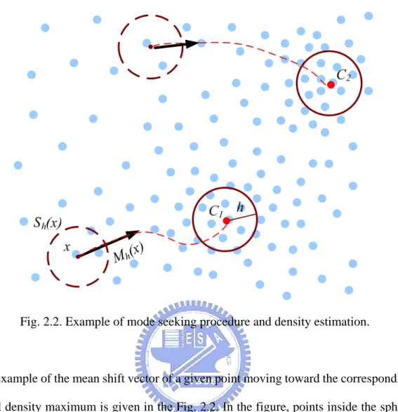
(22) corresponding 5-dimensional component in the feature space. This information is applied to mean shift vector to find the corresponding cluster mode. By calculating the mean shift vector, the location of the center of the hyper sphere is shifted iteratively according to x i +1 = x i + M h ( x i ) ,. (2.2). and the procedure will continued until the convergence is met at the corresponding mode for a given pixel. The convergence condition is xi+1 ≈ xi . Fig. 2.1 gives the flow chart of the mean shift filtering procedure. The output result is the smoothed image of the origin image.. Fig. 2.1. Flow of the mean shift filtering.. 6.

(23) Fig. 2.2. Example of mode seeking procedure and density estimation.. An example of the mean shift vector of a given point moving toward the corresponding local density maximum is given in the Fig. 2.2. In the figure, points inside the sphere Sh(x) with radius h around x is used to estimate the probability density function of x. The direction of the mean shift vector Mh(x) is computed and the new location is shifted iteratively until the point of convergence is reached. The convergence point always has the highest density in the feature space and is colored in red in Fig. 2.2. C1 and C2 are the center of the cluster 1 and cluster 2 in the example respectively.. For mean shift segmentation, an additional procedure that groups the clusters with mode distance smaller than hs in the spatial domain and hr in the range domain is performed after mean shift filtering. The parameters hs and hr are the radius of the window in the spatial and range domain respectively. Finally, an optional procedure 7.

(24) that eliminates regions with area smaller than M pixels is also performed to further improve the quality of the segmentation results. The flow chart of the mean shift segmentation is illustrated in Fig. 2.3.. Fig. 2.3. Flow of the mean shift segmentation.. An example of the mean shift segmentation is illustrated in Fig. 2.4 [6]. Fig. 2.4 (a) is a part of image data from Cameraman test image. Fig. 2.4(b) demonstrates the intermediate results during the mean shift filtering procedure. In the figure, each pixel is iteratively calculated using (2.1) and (2.2) to find the mean shift path represented as the block line. The black dots are the points of convergence for the corresponding pixels. After the mean shift filtering procedure, the smoothed image is demonstrated in Fig. 2.4 (c). Finally for the mean shift segmentation, clusters that are close to each other 8.

(25) in a predefined threshold are grouped together. Fig. 2.4(d) shows the final segmentation results using mean shift segmentation algorithm.. Fig. 2.4. Visualization of mean shift filtering and segmentation results for gray level data [6]. (a) Input image. (b) Mean shift mode seeking paths. (c) Mean shift filtering result. (d) Mean shift segmentation result.. 2.2. Watershed Algorithm Watershed segmentation is a popular and well known algorithm that extracts regions as catchment basins based on the concept of topography. The gradient image of the input image is used as the topographic surface in which the gradient value represents the altitude. The segmentation of an image finds the watershed line on the gradient image 9.

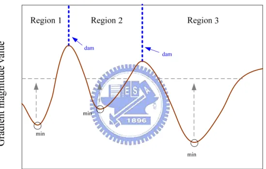
(26) and thus separates each region. There exist two approaches to implement watershed segmentation, one is the immersion-based method and the other is the toboggan-based method. The immersion-based watershed segmentation uses a bottom-up approach while the toboggan-based method uses a top-down approach to find the watershed line on the geography.. 2.2.1. Immersion-based Method. Fig. 2.5. Example of one dimensional signal using immersion-based watershed approach.. Immersion-based method can be explained as an iterative flooding approach. It can be thought as first pierce holes in each regional minimum of the topography surface. Then we slowly immerse this surface into the water. Starting from the regional minimum of the surface, the water will progressively flood up the catchment basins. While the waters from different catchment basins are about to merge, we build the dam to prevent 10.

(27) them from merging. In the end, each catchment basin is separated by the dam. The dams represent the watershed lines and catchment basins represent the segment regions. Take Fig. 2.5 for example. Three regional minimums are found and each of them corresponds to a catchment basin. Two dams which represent the watershed lines in the image are built to delimit the catchment basins. As a result, three segment regions are found.. There are two steps to implement the watershed algorithm proposed by Vincent and Soille [5], sorting and flooding procedure. Sorting procedure first sorts the pixels of an image in the increasing order of the gradient value for the purpose to access the pixels directly in a certain gray level. Then a flooding procedure is performed level by level starting from the minimum level to determine the watershed and catchment basins. At each gray level, pixels belong to the corresponding level h is first marked in label MASK. Then the neighboring status of those marked pixels is checked. If at least one of a neighbor of a pixel is labeled from the previous iteration, then the corresponding pixel is inserted in a first-in-first-out (FIFO) queue. Later, a recursive label propagation of each marked pixels in the FIFO is performed. If a pixel is adjacent to at least two different catchment basins, then the pixel is labeled as a watershed. If a pixel is only adjacent to one catchment basin, then it is labeled as the same label with the corresponding catchment basin. In the end, the remaining pixels still marked as MASK in the level h belongs to the regional minimum. The pixel and its connected components are given a new label as a new catchment basin. A pseudo code with more details of Vincent’s watershed segmentation algorithm is referred to [5].. 11.

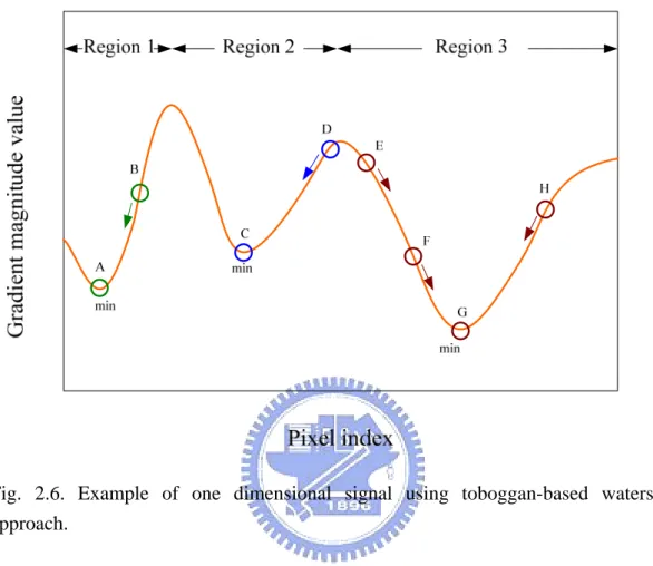
(28) 2.2.2. Toboggan-based Method. Fig. 2.6. Example of one dimensional signal using toboggan-based watershed approach.. Toboggan-based method can be thought as a rain drop sliding down from the hill by analogy. It tries to find out the downstream path where each rain drop slides down to a regional minimum of the topography surface. Each pixel represents a rain drop in the corresponding altitude of the topography surface. Pixels that slide down to the same regional minimum belong to the same catchment basin and a unique label is given. Fig. 2.6 gives a one dimensional example to describe the concept of the toboggan based method. The gradient value of pixel E’s right hand side is lower than the value of left-hand side, thus pixel E slides down in the right direction toward the regional minimum G. Pixel E, F and H slide down to the same regional minimum, thus belong to the same catchment basin. Finally, three regions are produced. Note that the 12.

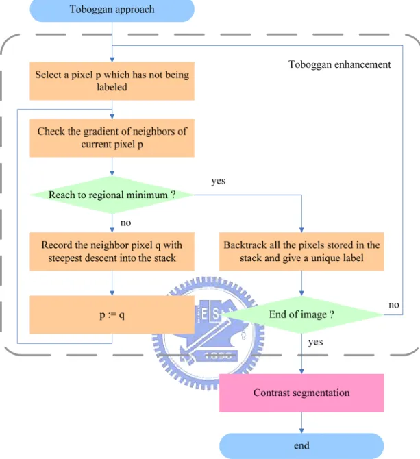
(29) toboggan-based algorithm is processed in a raster scan order. Thus in contrast with immersion-based algorithm, there is no need to perform an expensive sorting process which results in an irregular computing order. However, toboggan requires an additional backtracking procedure to solve the labeling problem in the algorithm.. The toboggan algorithm proposed by Fairfield [13] includes two steps, toboggan enhancement and contrast segmentation. In toboggan enhancement step, pixels slide down in the steepest descent according to the gradient value. In this step, pixels belonging to respective catchment basin are determined. This step usually produces an over segmentation result. To achieve better segmentation result, contrast segmentation is used as a post process to the segmentation image produced in the toboggan enhancement step. The contrast segmentation checks the color different between neighbors. If the color difference of two neighbor pixels is less than a pre-defined threshold, then two pixels is connected. This concept is similar to the region merge process. Fig. 2.7 shows the flow chart of the Fairfield’s toboggan based watershed segmentation.. Several toboggan-based approaches have been proposed to further improve the quality of the segmentation image based on Fairfield’s work. Readers can referred to [14] [15] for further detail information.. 13.

(30) Fig. 2.7. Flow chart of the Fairfield’s toboggan-based watershed segmentation.. 2.3. Markov Random Field based Algorithm 2.3.1. Markov Random Field Theory The following content of introduction on Markov random field theory in section 2.3.1 is 14.

(31) referenced from [16] [17]. Readers can refer to it for more details.. 2.3.1.1. Random Fields Many problems can be seen as labeling problems in terms of labels and states (or sites). A label is an event that may happen to a state and a set of discrete state is defined as DS = {0,1,..., m − 1} .. (2.3). A labeling problem chooses a label from the label set L = {0,1,..., l − 1} ,. (2.4). and assigns it to each of the states in DS. The value fi is regarded as a particular mapping of state i from DS to L and the set f = { f 0 , f1 ,..., f m −1} ,. (2.5). is called a labeling or a configuration of states in DS. The set of all possible configurations is called the configuration space and is defined as Ω= L. m. ,. (2.6). where m is the size of set DS.. Let F = {F0 , F1 ,..., Fm −1} be a family of random variables defined on the set of states DS where each random variable Fi take a value from the set of label L. This family F is called a random field. The event that Fi takes the value fi is denoted as Fi = fi. The probability that a random variable Fi takes a value fi is denoted as P ( Fi = f i ) and abbreviated as P ( f i ) . The notation ( F0 = f 0 , F1 = f1 ,..., Fm−1 = f m−1 ) or simply F = f denotes the joint event where f is a configuration of F and the joint probability is denoted as P(F = f ) , abbreviated P( f ) . 15.

(32) 2.3.1.2. Markov Random Fields In a regular lattice case, we consider DS as an image lattice X so that X = {x = ( p, q ) | ∀x ∈ DS} . Let Nx denotes the set of states neighboring x. N = {N x | ∀x ∈ X }. is said to be a neighboring system if it has the following two properties:. (i). A state is not neighboring to itself: x ∉ N x , ∀x ∈ X .. (ii). Neighboring is symmetry:. x ∈ N y ⇔ y ∈ N x , ∀x, y ∈ X. .. The definition of nth order neighborhood set and its neighborhood system is given as υ (np , q ) = {( k − p ) 2 + ( l − q ) 2 ≤ n ) | ∀ ( k , l ) ∈ X , ∀ ( p , q ) ∈ X }. υ. n. = {υ (np , q ) | ∀ ( p , q ) ∈ X }. .. ,. (2.7) (2.8). A first-order and a second-order neighborhood system are given as an example shown in Fig. 2.8. A first-order neighborhood system, also called a four neighborhood system, has four neighbors for each state in the regular lattice. A second-order neighborhood system, also called an eight neighborhood system, has eight neighbors for each state. Order that is higher than two is rarely used because it is complicated and requires a lot of computations in most applications.. 16.

(33) Fig. 2.8. Example of neighborhood system. (a) First-order neighborhood system. (b) Second-order neighborhood system.. A random field F is said to be a Markov Random Field (MRF) on X with respect to a neighborhood system N if and only if the following conditions are satisfied:. (i). Positivity : P( F = f ) > 0 for all possible configurations.. (ii). Markovianity : P( Fk = f k | Fi = f i , i ∈ X \ {k}) = P( Fk = f k | Fi = f i , i ∈ N k ) .. The notation \ denotes the exclusive operation, thus the notation i∈ X \ {k} denoted above means that i represents all possible states in set X but the state k. Thus { f i , i ∈ X \ {k}} denotes the set of labels of all states but k and { f i , i ∈ N k } denotes the set. of labels at the states neighboring k. Hence, the Markovianity condition describes the local characteristics of the random field that the probability of a state given a label in X is only affected by its neighborhood system. The positivity condition describes that all configurations are possible. 17.

(34) 2.3.1.3. Gibbs Random Fields A clique c is defined as any state in set X with all its possible pair neighbors in a neighborhood system. The set of all cliques is denoted as C. Fig. 2.9 gives examples of cliques for both the first order and second order neighborhood system on a regular image lattice. The first order neighborhood system contains two types of cliques, single-state clique and pair-state clique, as shown in Fig. 2.9 (a). A single-state clique contains only one state; a pair-state clique contains a pair of neighboring states; a triple-state clique contains a triple of neighboring states; and so on. The line connected the lattices in Fig. 2.9 indicates the neighboring connection between the states.. Fig. 2.9. Clique types for first order and second order neighborhood system. (a) First order neighborhood system. (b) Second order neighborhood system.. A random field F is said to be a Gibbs Random Field (GRF) on X with respect to a neighborhood system N if and only if its configurations follows a Gibbs distribution. A Gibbs distribution has the following form P( F = f ) =. 1 1 exp(− U ( f )) , Z T. (2.9). where T is a constant named as temperature, Z is a normalized constant called partition 18.

(35) function defined as Z=. ∑ exp( − T U ( f )) . 1. (2.10). f ∈Ω. Ω denotes the configuration space of all possible configurations defined in (2.6) and U ( f ) is the energy function that sums up the clique potential functions U c ( f ) of all. possible cliques c U( f ) =. ∑U ( f ) . c. (2.11). c∈C. The value of U c ( f ) depends on the local configuration on the clique c.. The joint probability P( F = f ) in (2.8) measures the probability of the occurrence of a particular configuration. From the definition above, it is clear that the lower the energy of a configuration has, the higher the probable a configuration is.. 2.3.1.4. Relation between MRF and GRF Markov random field follows the Markovianity property, thus it is characterized by the local property. Gibbs random field obeys a Gibbs distribution, thus it is characterized by the global property. The Hammersley-Clifford theorem [18] established the equivalence relationship of these two types of properties. The theorem states that a random field F is a MRF on X with respect to the neighborhood system N if and only if the random field F is a GRF on X with respect to the neighborhood system N. This equivalent provides a simple way to specify the local characteristic property of MRF by specifying the clique potential function which encodes a prior knowledge of interactions between neighbor nodes in image lattice. Thus the problem of finding the joint probability P( F = f ) of MRF becomes equivalent to first specifying the clique potential function U c ( f ) and then calculating the energy function U ( f ) as shown in 19.

(36) (2.10).. 2.3.1.5. MAP-MRF Framework The Bayesian approach can be used to solve the problem of image segmentation which can be thought as a labeling problem that gives a label in the segment label set L (2.4) to a state in set X. The result of the labeling problem is the segmentation image which is of interest. Let S be the set for a segment results based on the feature vector extracted from original image I. According to the Bayes’ rule, the posteriori probability can be presented as P(S = s | I = i) =. P( I = i | S = s) P(S = s) , P( I = i). (2.12). where P ( I = i | S = s ) represents the probability distribution of varying the segmentation result S for fixed image color information I and thus is called the likelihood of I. P(S = s) is the priori probability (prior) that defines the joint probability distribution of. neighboring segment labels. P ( I = i ) is the probability of the given image color information and it remains unchanged during the process, thus it is considered as a constant and the posteriori probability (2.12) is equivalent to P( S = s | I = i) ∝ P( I = i | S = s) P(S = s) .. (2.13). To obtain the most probable estimate of interest, a maximum a posteriori (MAP) approach is used. Taking the MAP of the posteriori probability (2.13) s MAP = arg max P ( S = s | I = i ) = arg max P ( I = i | S = s ) P ( S = s ) . s∈Ω s∈Ω. (2.14). The prior P(S = s) can be expressed as a MRF model. Thus it is served as a sum of the clique potential functions and can be expressed in the form similar to (2.9) as P( S = s) ∝ exp(− U (s )) . 20. (2.15).

(37) The Likelihood can also be expressed in terms of likelihood energy in the similar form of (2.10) as P( I = i | S = s) ∝ exp(− U (i | s )) .. (2.16). Thus the posteriori probability can be expressed in terms of energy function as P( S = s | I = i) ∝ exp(− U (s | i )) ,. (2.17). U (s | i ) = U (i | s ) + U (s ) .. (2.18). where. Thus from (2.17) and (2.18), the MAP of the posteriori probability in (2.14) is equal to find the minimize of the posterior energy function sˆ = arg min U (s | i ) . s∈Ω. (2.19). With the use of MAP-MRF approach, a segmentation problem which is also referred to the labeling problem can be solved for the following steps. First, define the neighborhood system and the set of cliques. Then define a clique potential function and the likelihood energy function for the estimation of (2.15) and (2.16) respectively. Finally, choose an optimization algorithm to find the optimized MAP solution of the posteriori probability (2.14) or (2.17).. 2.3.2. Application in Segmentation The applications of MRF model have been widely use in a variety of image processing tasks such as image restoration, edge detection, motion analysis and image segmentation. In this section, we will focus on the MRF model established in the field of image segmentation.. 21.

(38) 2.3.2.1. Deng’s Work Deng’s work [8] proposed a simple MRF model for unsupervised image segmentation. The segmentation problem can be expressed in the Bayesian framework (2.12) where the posteriori probability P( S = s | I = i ) consists of two components, a region labeling component and a feature modeling component. These two components can be formulated in the MRF model. The prior P(S = s) is referred to the region labeling component and the energy function of the prior using the pairwise multi-level logistic (MLL) model is given as U (s ) =. ⎡. ∑ ⎢⎢ β ∑ δ (s. q∈ X. ⎣. q∈ N ( p ). ⎤. p , sq. )⎥ ,. (2.20). ⎥⎦. where β is a weighting constant which can be specified a priori, sp is a labeling condition of state p in the set of image lattice X and a clique potential function is defined as s p = sq. ⎧⎪ 1, ⎪⎩− 1,. δ (s p , s q ) = ⎨. s p ≠ sq. (2.21). .. Deng assumes that the probability distribution of all feature data for one segment region is a Gaussian distribution. Based on this assumption, the likelihood energy which is referred to the feature modeling component that describes the features of an image is defined as U (i | s ) =. ∑∑ S. where. ip. (. ). ⎧ ⎡ i −μ 2 ⎪ p l + log 2π σ l ⎨ ⎢ 2 ⎪⎩ p∈X ⎢⎣ 2(σ l ). (. ⎤⎫. )⎥⎥⎪⎬ . ⎦ ⎪⎭. (2.22). is the feature information of state p extract from the original image I, μ l. and σ l are the mean and standard deviation for the segment region labeled l. Note that the number of segment regions is assumed to be known in prior. After defining the components, the energy of the posterior probability P(S = s | I = i) is then defined as 22.

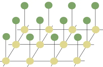
(39) U (s | i ) = α (t )× U (i | s ) + U (s ). (2.23). where α (t ) is the variable weighting parameter. Deng claims that with this function-based parameter gives the individually contribution of the two components to the entire energy U (s | i) , the proposed simple MRF model is able to automatically estimate model parameters and produce accurate unsupervised segmentation results using expectation-maximization (EM) algorithm and fast simulated annealing (SA).. 2.3.3. Inference Algorithm Using Loopy Belief Propagation There are several methods to solve the MAP-MRF problem such as simulated annealing (SA) [7], iterated conditional modes algorithm (ICM) [19], belief propagation (BP) [11], and graph cut method (GC) [20]. Among all, we are interested in the loopy belief propagation that applies Pearl’s algorithm [10] to the graph with loops or undirected graphs. A Markov network is an undirected graph in the literature of probabilistic graph models [21], where the nodes represent variables and arcs which connect the neighboring nodes represent compatibility relations between neighboring nodes. Fig. 2.10 shows an example of an undirected graphical model. Yellow nodes represent the hidden variables and green nodes represent the observed variables. In this section, we will focus on the loopy belief propagation algorithm. We will refer loopy belief propagation as belief propagation for brevity.. 23.

(40) Fig. 2.10. An undirected graphical model with hidden variables and observed variables.. Pearl’s algorithm is an exact inference algorithm for graphs without loops or directed graphs. For the graphs with loops or undirected graphs such as the image lattice structure, belief propagation is not guaranteed to find the global optimal solution. Despite of this, several applications have been successfully used in applications such as the one with stereo vision [11]. Belief propagation iteratively propagates messages in the Markov network. Let. (. m tpq+1 x p , x q. ) be the message that propagates from node xp to xq. in iteration t+1, and is defined as. (. ). (. ) (. mtpq+1 x p , xq ← κ maxψ pq x p , xq mtp x p , i p. where ψ. pq. (. m tp x p , i p. xp. ) ∏ mkpt (xk , x p ). ) is the message from observed node ip to node xp in iteration t,. (x p , x q ) is the compatibility matrix with size L × L between node xp and its neighbor. nodes xq. L is the size of all possible labels. Note that both message. (. (2.24). x k ∈N ( x p ) \ x q. m tp x p , i p. (. m tpq+ 1 x p , x q. ) and. ) are vectors with L elements. The belief of node xp is computed as follows:. ( ). (. b p x p ← κm p x p , i p. ) ∏ mkp (xk , x p ) , xk ∈N ( x p ). 24. (2.25).

(41) ( ). xMAP = argmaxbp x p , p xp. where. κ. (2.26). is the normalized constant. Note that belief. ( ) is also a vector with L. bp x p. elements. Fig. 2.11 gives an example of local message passing in the Markov network. The message propagates from node x1 to node x2 is m1,2 ← κ maxψ 12 (x1 , x2 )m1m3,1m4,1m5,1 . x1. The belief at node x2 is. b2 ← κm2 m1, 2 m6 , 2 m7 , 2 m8, 2 .. i1 m1. i2 m2. x4. x6. m4,1 m3,1. m6,2. m1,2. x3. x1. x7. x2 m7,2. m2,1 m8,2. m5,1 x5. x8. Fig. 2.11. Local message passing in a Markov Network [11]. The belief propagation with max-product update rule maximizes the joint posterior probability P( X = x | I = i) with the MRF model in the following steps: 1.. Initialize messages. (. m pq x p , x q. ) and. (. m p x p , iq. ) of each node to a constant and. the observed values calculated from the likelihood function respectively. 2.. Update messages of each node iteratively using equation (2.24).. 3.. Computes and determines the belief of the corresponding nodes using equation (2.25) and (2.26) at the end of the BP algorithm.. 25.

(42) 26.

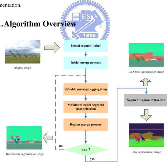
(43) Chapter 3. Color Image Segmentation Algorithm Using MRF Model In this chapter, we propose a color image segmentation method with a new MRF modeling of color image segmentation and a local belief aggregation (LBA) algorithm to estimate the MAP inference. The proposed MRF models the likelihood and prior probability based on the concept of the intra and inter region constraint respectively. The LBA algorithm, which is inspired by the original BP and DQ, is proposed to cope with the problems of the large number of segment labels existing in color image segmentation.. 3.1. Algorithm Overview. Fig. 3.1. Flow of image segmentation using local belief aggregation. 27.

(44) Fig. 3.1 illustrates the flow of the image segmentation using local belief aggregation. Before using local belief aggregation algorithm to optimize the total energy, an initial segment label is assigned. In this step, a unique segment label is first assigned to each pixel in the test image. If there are |I| pixels in the image, there would be |I| segment labels in the initial segmentation image. Note that there is no restriction on the quality of the initial segment map. However, a more accurate initial guess will lead to faster convergence of the following local belief aggregation algorithm. Besides, segment labels can also be used as the seeds for segment regions. Therefore, an initial merge process is applied to the initial segmentation image. After the initial merge process, the proposed local belief aggregation (LBA) is performed iteratively to find the segmentation image. We model the image segmentation as a labeling problem using a four-connect MRF, in which each node corresponds to a pixel and each state corresponds to a segment label. The LBA consists of reliable message aggregation, maximum belief segment state selection, and region merge process. First, reliable message aggregation aggregates reliable message information from the neighboring nodes of each node in the MRF. At each node, the belief value of each segment state is computed using the reliable message aggregated in the previous step. The segment state with the maximum belief value is chosen. For each node, the corresponding label of the chosen segment state is selected as the segment label. After the maximum belief segment state selection, a region merge is applied to further improve the segmentation image quality. The LBA steps are iteratively performed until convergence or a preset iteration limit is reached. After the LBA, segment region extraction is performed to output the final segmentation image. The segment region extraction assigns a new unique segment label to each region using connected component. This is an option step in the LBA algorithm. Note that we perform two different kinds of initial merge process, 28.

(45) a local partial merge and a global merge, as an initial segment map for the following LBA. A local partial merge that only considers spatial and color information in a 3×3 sliding window is used for the four-window based LBA. A global merge is used for one-window based LBA.. 3.2. CIE L*a*b* Color Space In the proposed color image segmentation algorithm, a precise estimation of color distance is important. Thus a proper choice of color space is important in our case. We adopt the CIE L*a*b* color space from all the existing color space for two reasons: (1) approximately uniform color scale, (2) similar to human visual perception.. 3.2.1. Introduction The L*a*b* color space is developed by the CIE to be approximately perceptually uniform. Color difference between points in the color space corresponds to the visual difference between the colors of the points. The L* axis represents the lightness (luminance) in this color space with white at L* = 100 and black at L* = 0. The a* and b* axes represents color component while a* encodes the red-green sensation and b* encodes the yellow-blue sensation. Positive a* axis indicates amounts of red color and negative a* axis indicates amounts of green color while positive b* axis indicates amounts of yellow color and negative b* axis indicates amounts of blue color. Note that there is no specific numerical limit for these two color components. Fig. 3.2 illustrates a brief plot of the CIE L*a*b* color space.. 29.

(46) Fig. 3.2. CIE L*a*b* color space.. 3.2.2. Color Transform from RGB to CIE L*a*b* Color transformation from RGB to CIE L*a*b* color space is done by the following two steps. First we transform RGB to CIE XYZ space. This transformation is made by ⎡ X ⎤ ⎡0.412453 0.357580 0.180423⎤ ⎢Y ⎥ = ⎢0.212671 0.715160 0.072169⎥ ⎢ ⎥ ⎢ ⎥ ⎢⎣Z ⎥⎦ ⎢⎣0.019334 0.119193 0.950227⎥⎦. ⎡R ⎤ ⎢G⎥. ⎢ ⎥ ⎢⎣ B ⎥⎦. (3.1). Then we transform the resulting CIE XYZ space to CIE L*a*b* space. The transformation is defined by ⎡ ⎛Y L* = 116 × ⎢ f ⎜⎜ ⎣⎢ ⎝ Yn. ⎞⎤ ⎟⎟ ⎥ − 16 , ⎠ ⎦⎥. (3.2). ⎡ ⎛ X ⎞ ⎟⎟ − a* = 500 × ⎢ f ⎜⎜ ⎣⎢ ⎝ X n ⎠. ⎛ Y ⎞⎤ f ⎜⎜ ⎟⎟⎥ , ⎝ Yn ⎠⎦⎥. (3.3). ⎡ ⎛Y b* = 200 × ⎢ f ⎜⎜ ⎣⎢ ⎝ Yn. ⎛ Z f ⎜⎜ ⎝ Zn. ⎞⎤ ⎟⎟⎥ , ⎠⎦⎥. (3.4). where. 30. ⎞ ⎟⎟ − ⎠.

(47) ⎧1 ⎪⎪t 3 f (t ) = ⎨ ⎪7.787 × t + 16 ⎪⎩ 116. if t > 0.008856,. (3.5). if t ≤ 0.008856.. ( X n , Yn , Z n ) : refernece white. 3.2.3. Color Difference Color difference between two points in the CIE L*a*b* space is given by the Euclidean distance formula * ΔEab. 1 * 2⎤2. ( ) + (Δa ) + (Δb ) ⎥⎦. = ⎡ ΔL ⎢⎣. * 2. * 2. ,. (3.6). where the differences in lightness (ΔL* ) , red-green sensation (Δa* ) and yellow-blue sensation (Δb* ) is defined as ΔL* = L*1 − L*2 , Δa * = a1* − a 2* , Δb = *. b1*. (3.7). − b2* .. 3.3. MRF Model Formulation According to the Bayes’ theorem, the posterior probability of a segmentation image S, given the image information I, can be represented as (2.12) and simplified to (2.13) since P ( I = i ) in (2.12) can be considered as a constant. In this section, we formulate the MRF model of the likelihood P( I = i | S = s) and the prior P(S = s) in order to further estimate the posterior probability to obtain the segmentation result.. 3.3.1. Likelihood and Prior We define the likelihood P ( I = i | S = s ) as 31.

(48) P( I = i | S = s) ∝. ∏exp(−F ( x, s ,i)) ,. (3.8). x. x∈I. where F ( x, s x , i) is the cost function of node x with segment label sx given the observation I. The prior P(S = s) is defined as P(S = s ) ∝. ∏ ∏exp(−η (s , s ,γ (s , s ))) , x. y. x. (3.9). y. x∈I y∈N ( x ). where η ( s x , s y , γ ( s x , s y )) is the clique potential function of segment label sx and sy in which node y is the neighbor of node x. γ (sx , s y ) is the line process which penalizes the clique potential according to the relationship between segment label sx and sy. By combining (2.13), (3.8) and (3.9), the basic model (2.12) of the image segmentation becomes P(S = s | I = i ) ∝. ∏ exp(− F (x, s , i))∏ ∏ exp(−η (s , s , γ (s , s ))) . x. x∈I. x. y. x. y. (3.10). x∈I y∈N ( x ). 3.3.2. Model Approximation To estimate the optimal solution of a MRF model, the maximum a posteriori (MAP) approach is used. Taking the MAP of (3.10) gives max{P( S = s | I = i)} ⎧⎪ = max⎨ exp(− F (x, s x , i )) ⎪⎩ x∈I x∈I. ⎫⎪ exp − η s x , s y , γ s x , s y ⎬ ⎪⎭ y∈ N ( x ). ∏∏ ( (. ∏. (. ⎧ ⎡ ⎛ ⎪ = max⎨ exp ⎢− ⎜ F (x, s x , i ) + η sx , s y , γ sx , s y ⎢ ⎜ ⎪⎩ x∈I ∈ ( ) y N x ⎝ ⎣. ∑(. ∏. (. ⎧ ⎡ ⎪ ⎢ F ( x, s x , i ) + = exp⎨− min η sx , s y , γ sx , s y ⎪⎩ x∈I ⎢ y ∈ N ( x ) ⎣. ∑. ∑(. (. ⎞⎤ ⎫. ))⎟⎟⎥⎥ ⎪⎬. ))). (3.11). ⎠⎦ ⎪⎭. ⎤⎫. ))⎥ ⎪⎬. ⎥⎦ ⎪ ⎭. The question here is to determine the definition of the cost function F ( x, s x , i) and the clique potential function η ( s x , s y , γ ( s x , s y )) in the likelihood and the prior respectively. Haralick and Shapiro [22] pointed out two criteria on the characteristics of segments in a good segmentation image. One measures the intra region uniformity and the other 32.

(49) measures the inter region disparity. These two criteria show consistency with the likelihood and prior function. Thus we model the likelihood and prior function based on the intra and inter region criteria respectively. Specifically, the definition of intra and inter region energy defined in [23] is adopted and modified. We define the cost function and the clique potential function as. (. F (x, s x , i ) = u ix − s x. L*a*b*. η (s x , s y , γ (s x , s y )) = u ⎛⎜ th v − s x − s y ⎝. ). − thv ,. (3.12). (. ⎞⎟ × γ s , s x y. L*a *b* ⎠. ),. (3.13). where s x and sy represents the average color of segment label sx and sy respectively, thv denotes the threshold for visible color difference,. L*a*b*. denotes the color. difference in the CIE L*a*b* space and γ (s x , s y ) denotes the relation between a pair of segment labels and is defined as sx ≠ s y. ⎪⎧1, ⎪⎩0,. γ (s x , s y ) = ⎨. sx = s y. .. (3.14). Thus, with the above definition of cost function and clique potential function, (3.11) can be rewritten as max{P(S = s | I = i )} ⎧ ⎡ ⎤ ⎫⎪ ⎪ ⎢ F ( x, s x , i ) + = exp ⎨− min η sx , s y ,γ sx , s y ⎥⎬ ⎥⎪ ⎪⎩ x∈I ⎢ y∈N ( x ) ⎣ ⎦⎭ ⎧ ⎡ ⎪ = exp ⎨− min ⎢ F (x, s x , i ) + η sx , s y ,γ sx , s y ⎢ x∈I ⎪⎩ x∈I y∈N ( x ) ⎣. ∑. ∑(. ∑. ∑∑(. [. (. = exp{− min Eintra × I + Einter × C × I. = exp{− min [Ecw ]}. )). (. ]}. ⎤⎫. ))⎥ ⎪⎬ ⎥⎪ ⎦⎭. (3.15). where Ecw is the weighted sum of intra-region visual error (Eintra) and inter-region visual error (Einter) whose definition from [23] are. Eintra =. ∑ u ⎛⎜⎝. ix − s x. x∈ I. I. 33. L * a *b *. − thv ⎞⎟ ⎠. ,. (3.16).

(50) ∑ ∑ α (s , s )× u⎛⎜⎝ th x. Einter =. y. v. − sx − s y. x∈I y∈N ( x). ⎞⎟. L*a*b* ⎠. ,. C× I sx ≠ s y. ⎧⎪1, ⎪⎩0,. α (s x , s y ) = ⎨. sx = s y. (3.17). ,. (3.18). t>0 . t≤0. ⎧1, u (t ) = ⎨ ⎩0,. (3.19). |I| represents the total number of pixels in an image, C is a weighting constant. From the inference of (3.15), it is obvious that estimating a MAP of P(S = s | I = i) with the definition of cost function and clique potential function in (3.12) and (3.13) is equivalent to obtaining the minimum energy of Ecw. This equivalence is what we desired since [23] claimed that lower Ecw implies better image segmentation results.. In addition to the definition of intra-region visual error and inter-region visual error defined in (3.16) - (3.19), Chen also claims that the modified version of these two terms that further include the color distance values can also give a quantitative evaluation of the segmentation images [24]. The definition of the modified intra-region visual error (MEintra) and modified inter-region visual error (MEinter) is given as follows. MEintra =. ∑ ⎧⎨⎩u⎛⎜⎝ x∈I. L * a *b *. − thv ⎞⎟ × ⎛⎜ ix − s x ⎠ ⎝. L* a *b *. − thv ⎞⎟⎫⎬ ⎠⎭. I. ∑ ∑ ⎧⎨⎩α (s , s )× u⎛⎜⎝ th x. MEinter =. ix − s x. y. v. − sx − s y. x∈I y∈N ( x ). ⎞⎟ × ⎛⎜ th − s − s x y ⎝ v. L*a*b* ⎠. ,. ⎧⎪1, ⎪⎩0,. , sx ≠ s y sx = s y. ⎧1, u (t ) = ⎨ ⎩0,. ,. t>0 . t≤0. Again, if we define the cost function and the clique potential function as 34. ⎞⎟⎫ ⎬. L*a*b* ⎠⎭. C× I. α (s x , s y ) = ⎨. (3.20). (3.21) (3.22) (3.23).

(51) F (x , s x , i ) = u ⎛⎜ i x − s x ⎝. L * a *b *. η (s x , s y , γ (s x , s y )) = u ⎛⎜ th v − s x − s y ⎝. L * a *b *. − th v ⎞⎟ × ⎛⎜ i x − s x ⎠ ⎝. L * a *b *. ⎞⎟ × ⎛⎜ th − s − s x y ⎠ ⎝ v. sx ≠ s y. ⎪⎧1, ⎪⎩0,. γ (s x , s y ) = ⎨. sx = s y. − th v ⎞⎟ ⎠. L * a *b *. ,. (3.24). (. ⎞⎟ × γ s , s x y ⎠. ),. ,. (3.25) (3.26). and take the MAP of (3.10), the same conclusion will make as in (3.15).. Although maximizing the posterior defined by (3.12), (3.13) and (3.24), (3.25) can minimize Ecw as shown in (3.15), an energy distribution that is proportional to color difference is considered to be a more suitable measure. Thus, based on the property of intra region and inter region, we re-formulate the cost function and clique potential function as F ( x, s x , i ) = i x − s x. η (s x , s y , γ (s x , s y )). L*a *b*. ,. ⎧ s −s ⎪ x y L*a*b* =⎨ ⎪ths − s x − s y L*a*b* ⎩. (3.27) sx = s y sx ≠ s y. ,. (3.28). where ths denotes the threshold for maximum difference of average segment label color between two segment labels. From the empirical experiment results, we select threshold ths to be 150 to simplify the problem of finding different threshold for different test images. Thus, in the case of different segment labels detected in (3.28), we truncate the value of clique potential function to zero if s x − s y larger than the 150, which is the predefined threshold ths as shown in Fig. 3.3.. 35. L∗a∗b∗. is.

(52) η(sx,sy,γ(sx,sy)). 160 150 140 130 120 110 100 90 80 70 60 50 40 30 20 10 0 0. 50. 100. sx − sy. 150. 200. 250. L ∗ a ∗b ∗. Fig. 3.3. Relation between the value of clique potential function and the value of difference of average segment label color for two different segment labels.. Our formulation adopts Gaussian-like color distribution model; however, [25] has pointed out that such model may not always be true. To accommodate the distribution deviations, two discontinuity preserving robust functions derived from the Total Variance (TV) model [26] are applied to the cost and clique potential function. P( S = s | I = i ) ∝. ∏ exp(− ρ (s ))∏ ∏ exp(− ρ (s , s )) , l. x. p. x∈I. x. y. (3.29). x∈I y∈N ( x ). where the robust functions are defined as ⎡. ⎛. ⎢⎣. ⎝. ρ l (s x ) = − ln ⎢(1 − el ) exp⎜⎜ − ⎡. (. ⎛ η sx , s y , γ sx , s y ⎜ σp ⎝. ρ p (s x , s y ) = − ln ⎢(1 − e p )exp⎜ − ⎢ ⎣. (. ⎤ F ( x, s x , i ) ⎞ ⎟ + el ⎥ , ⎟ σl ⎥⎦ ⎠. )) ⎞⎟. ⎤ + ep ⎥ . ⎟ ⎥ ⎠ ⎦. (3.30). (3.31). Note that parameter σ and e control the sharpness and upper-bound of the function respectively. In our experiment, the parameter σ and e is set to be 2.0 and 0.01 respectively for both cost function and clique potential function.. Finally, the posterior P (S = s | I = i ) can be factorized into the following form 36.

(53) P(S = s | I = i ) ∝. ∏ψ. x. x∈I. where ψ x (s x , ix ) ∝ exp(− ρ l (s x )) is ψ xy (s x , s y ) = exp (− ρ p (s x , s y )) is. the. (sx , ix )∏. ∏ψ (s , s ) , xy. x. (3.32). y. x∈I y∈N ( x ). local. evidence. for. node. x,. and. the compatibility matrix between node x and its neighbor. nodes y.. 3.4. Local Belief Aggregation To efficiently estimate the MAP of the posterior probability (3.32), a local belief aggregation (LBA) is proposed. Although belief propagation (BP), which is a linear time algorithm proportional to the number of hidden nodes [11], can also be used to solve the MAP problem, there are some difficulties to directly apply BP algorithm in the proposed MRF-based segmentation model. The enormous size of segment labels not only results in heavy computational burden but also leads to a huge memory storage requirement. Both of these constraints restrict the use of BP in color image segmentation. Thus, a local belief aggregation which is modified from the original BP algorithm is proposed to find the MAP segmentation image.. 3.4.1. Reliable Message Aggregation Reliable message aggregation is the first step in the LBA. The reliable message aggregation restricts the number of segment state’s message to be aggregated from the neighbor nodes. That is, only a limited number of the most probable segment states, which we considered to be reliable, can send out messages. To decide the most probable segment states, a local search window approach is used. Here we introduce 37.

(54) two methods of using local search window to send out the reliable messages. In section 3.4.1.1, we will introduce the four-window based local search window method. In section 3.4.1.2, one window-based local search window method is proposed to further reduce the computational complexity than the previous method.. 3.4.1.1. Four-window Based Local Search Window i6 Local search window at x6 (3x3). m6 i2. i1 m1. m2. x4. i7 x6. i8. Local search window at x7 (3x3). m7. m6,2. m1,2 x3. x1. x7. x2 m8. m7,2 m8,2. x5. x8. Local search window at x1 (3x3). Local search window at x8 (3x3). Fig. 3.4. Reliable message aggregation using four local search windows.. Fig. 3.4 shows the concept of four-window based local search window. In this method, each neighboring node has its corresponding local search window in a preset size. For example, nodes x1, x6, x7 and x8 have their corresponding 3×3 local search window shown in Fig. 3.4. During the procedure, the message of node x1 will be calculated and decided using the local search window center at node x1. Once the reliable message is ready, message of node x1 will propagate to the current node x2. The same action is performed for node x6, x7 and x8 at the same time to propagate the reliable messages to node x2. 38.

(55) Let m be the number of all the segment states appeared in the local search window. All messages from these m segment states will be calculated. Let mxy(sx,sy) be the message from node x to node y, and is defined as mxy (sx , s y ) ← κ maxψ xy (sx , s y )υx (sx , sz )mx (sx , ix ) sx. ∏. rkx (sk , ik ) sk ∈N ( s x ) \ s k. ,. (3.33). where υ x (s x , s z ) is the spatial function considering the spatial relationship of the m segment states in node x and the segment state of node z in the corresponding local search window. Here our spatial function is simply defined as the reciprocal of the spatial distance υ x (s x , s z ) =. 1 , Eu d (s x , s z ). (3.34). where Eu d (s x , s z ) is the Euclidean distance between the segment state of node x and the segment state of node z. mx ( s x , ix ) = ψ x ( s x , ix ) is the message from observed node ix to node x and rks ( s k , ik ) = ψ k ( s k , ik ) is the message from node k to node x. If the number of possible segment state m in the local search window is larger than a preset number of reliable segment states n, then only the message of the most probable n segment states out of the m segment states can be transferred according to the message value calculated by (3.33). Higher message value represents higher probability. The other (m-n) number of less probable segment states will be discarded for current node calculation. From (3.33), it is obvious that the message can be calculated on-the-fly, hence no memory storage for previous iteration’s messages is required any more.. 39.

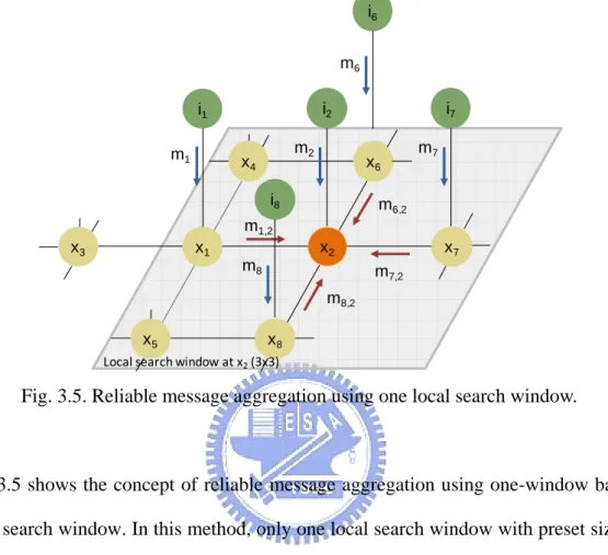
(56) 3.4.1.2. One-window Based Local Search Window i6 m6 i2. i1 m1. m2. x4. i7 x6. i8. m7. m6,2. m1,2 x3. x1. x7. x2 m8. m7,2 m8,2. x5. x8. Local search window at x2 (3x3). Fig. 3.5. Reliable message aggregation using one local search window.. Fig. 3.5 shows the concept of reliable message aggregation using one-window based local search window. In this method, only one local search window with preset size is required to determine the reliable messages. Let m be the number of all the segment states appeared in the local search window. All messages from these m segment states will be calculated using the same equation (3.33). All the m number of messages in four directions will be considered as reliable messages and will aggregate into the node without being discarded to provide reliable information for further belief value calculation.. 40.

(57) 3.4.2. Maximum Belief Segment State Selection The maximum belief segment state selection is performed after the reliable message aggregation. During this procedure, the belief of the node x will be estimated and the segment state with the maximum belief will be selected. The belief is computed as follows: bx (s x ) ← κmx (s x , ix ). ∏m. kx. (sk , s x ) ,. (3.35). sk ∈N ( sx ). s xMAP = arg max b x (s x ) .. (3.36). sx. Note that in the four-window based local search window method, there is a chance that some of the segment state’s message is missing while computing the belief value. This is due to the restriction on the number of the reliable message to be sent from the neighboring nodes with their corresponding local search window. To remedy this, the missing message belonging to a specific segment state of the corresponding neighboring node is re-computed. For one-window based local search window method, there is no need to re-compute since no restriction on the number of the reliable message is performed.. 41.

(58) i4 m4 i3. i1. m3. i2. m1. x4. x6 m2. r4,1. i5 r3,1. m6,2. m1,2. x3. x1. x7. x2 m7,2. m5 m8,2. r5,1 x5. x8. Local search window at x1 (3x3). Fig. 3.6. Four-window based local reliable message aggregation in a Markov network.. i4 m4 i3. i1. m3. m1. i2 x4. x6 m2. r4,1. i5 r3,1. m6,2. m1,2. x3. x1. x7. x2 m7,2. m5 m8,2. r5,1 x5. x8. Local search window at x2 (3x3). Fig. 3.7. One-window based local reliable message aggregation in a Markov network.. Fig. 3.6 and Fig. 3.7 demonstrate the example of the message aggregation in four-window based local search window and one-window based local search window with belief calculation in a Markov network respectively. In both figures, green nodes 42.

(59) represent the observed variables. Yellow and orange nodes represent the hidden variables. Gray region represents a preset size of local search window which is 3 × 3 in the example centered at nodes x1 and x2 in the four-window based method and one-window based method respectively. Reliable message aggregate from node x1 to x2. is m1, 2 ← κ maxψ 12 (s x1 , s x2 )υ1 (s x1 , s xz )m1m3 m 4 m5 . s x1. The. belief. at. node. x2. is. b x 2 ← κ m 2 , m 1, 2 , m 6 , 2 , m 7 , 2 m 8 , 2 .. 3.4.3. Region Merge Process The initial guess of the segmentation image may consist of a large number of unnecessary segment labels. As a consequence, we would be using more than one segment labels to represent a region. This would prevent the overall energy from converging. For the above reason, redundant segment labels should be pruned. Hence, a region merging process is inserted in the end of each iteration. At the end of each iteration, the average color difference of two neighboring segment regions is checked. If the color difference is smaller than a pre-defined threshold, the two segment regions should be the same. In other words, the two different segment labels represent the same region. In this case, one of the two segment labels is replaced by the other.. Additional region merging based on the area of regions is also performed to further improve the quality of the segmentation image. In the four-window based local search window, the additional region merging is performed at the first and last iteration of the LBA as shown in Fig. 3.8. In the one-window based local search window, the additional region merging is performed twice, after the region merge process at the first and last iteration of the LBA as shown in Fig. 3.9. In this additional region merge, 43.

(60) segment regions with an area smaller than a predefined area are merged into their neighboring segment regions that have the smallest color distance with an area larger than a predefined number. The predefined areas are both 20 pixels in our case.. Fig. 3.8. Region merge process in four-window based method.. 44.

(61) Region merge process. Region merge based on color difference. First iteration or last iteration ?. no. yes. Region merge based on area. Fig. 3.9. Region merge process in one-window based method.. 3.4.4. Convergence of Local Belief Aggregation Similar to BP, there is no theoretical proof to guarantee the convergence of the proposed local belief aggregation method. However, we suspect that LBA is likely to achieve convergence in practice. We use empirical result to demonstrate LBA’s convergence trend. For the purpose of minimizing the energy term Ecw, it is reasonable that the convergence of the energy term Ecw could imply the convergence of the proposed local belief aggregation algorithm. Fig. 3.10 shows the Ecw curve for the test image 253055 from Berkeley Segmentation Database [27]. As we can see, after several iterations of estimating posterior probability by LBA, the energy term Ecw oscillates around the value 0.136. Hence, we believe that the LBA tends to converge as the Ecw energy term is converging.. 45.

(62) 0.8. test image 253055. 0.7. Ecw energy. 0.6 0.5 0.4 0.3 0.2 0.1 0 0. 10 20 30 40 50 60 70 80 90 100 110 120 130 140 150 Iteration. Fig. 3.10. Ecw convergence of four-window based LBA. In addition to the Ecw curve, another empirical method to demonstrate the convergence trend is to check the results of the segmentation image subjectively. If the result of the segmentation images is convergence, than we believe that the LBA also tends to converge. For test images we use, this convergence tend is guaranteed so far.. 3.5. MRF Model Comparison We suspect that the MRF model using (3.12), (3.13) and (3.24), (3.25) is not suitable for the proposed algorithm for two reasons. First, two-value model provides less information for a labeling problem such as the image segmentation problem. An energy distribution proportional to color difference can give a Gaussian-like measure and thus is considered to be a more suitable measure. Second, in the proposed LBA algorithm, the region merge process will merge two neighbor segment regions with 46.

(63) average color distance smaller than a predefined threshold. If the region merge threshold is selected larger than or equal to the visible color difference threshold thv , then the input of the unit step function in (3.13) and (3.25) will always be smaller or equal to zero. From (3.19), this will cause the results of unit step function that appears in (3.13) and (3.25) to always be equal to zero. Thus the concept of unit step function is considered not suitable for the region merge process of the proposed LBA. Fig. 3.11 shows the LBA results using (3.12), (3.13) and (3.24), (3.25) respectively. The region merge threshold is chosen to be 2 in order to be less than the threshold for visible color thv and we run the LBA for 5 iterations. All two images perform bad segmentation results, both methods cannot successfully segment out giraffes of the test image 253055; however, Fig. 3.11 (b) is better than Fig. 3.11 (a) among the two. We suspect that this is because MRF model used in the Fig. 3.11 (b) has include the color distance values which is better than the two-value MRF model used in Fig. 3.11(a). From the above reasons and the empirical experiment, (3.27) and (3.28) is adopted as the energy of the likelihood and the prior respectively. The segmentation results of the selected MRF model will be demonstrate in the next section and throughout the thesis.. Fig. 3.11. Segmentation results with different MRF model using LBA algorithm. (a) MRF model using (3.12) and (3.13). (b) MRF model using (3.24) and (3.25). 47.