Shortest service location model for planning waste pickup locations

This article was downloaded by: [National Chiao Tung University 國立交通大學]

On: 30 April 2014, At: 23:21

Publisher: Taylor & Francis

Informa Ltd Registered in England and Wales Registered Number: 1072954 Registered office: Mortimer House,

37-41 Mortimer Street, London W1T 3JH, UK

Journal of the Air & Waste Management Association

Publication details, including instructions for authors and subscription information:

http://www.tandfonline.com/loi/uawm20

Shortest Service Location Model for Planning Waste

Pickup Locations

Jehng-Jung Kao

& Tsung-I Lin

a

Institute of Environmental Engineering , National Chiao Tung University , Hsinchu , Taiwan,

Republic of China

b

Axtronics Information Appliances Innovator Co. , Hsinchu , Taiwan, Republic of China

Published online: 27 Dec 2011.

To cite this article: Jehng-Jung Kao & Tsung-I Lin (2002) Shortest Service Location Model for Planning Waste Pickup Locations,

Journal of the Air & Waste Management Association, 52:5, 585-592, DOI:

10.1080/10473289.2002.10470807

To link to this article: http://dx.doi.org/10.1080/10473289.2002.10470807

PLEASE SCROLL DOWN FOR ARTICLE

Taylor & Francis makes every effort to ensure the accuracy of all the information (the “Content”) contained

in the publications on our platform. However, Taylor & Francis, our agents, and our licensors make no

representations or warranties whatsoever as to the accuracy, completeness, or suitability for any purpose of the

Content. Any opinions and views expressed in this publication are the opinions and views of the authors, and

are not the views of or endorsed by Taylor & Francis. The accuracy of the Content should not be relied upon and

should be independently verified with primary sources of information. Taylor and Francis shall not be liable for

any losses, actions, claims, proceedings, demands, costs, expenses, damages, and other liabilities whatsoever

or howsoever caused arising directly or indirectly in connection with, in relation to or arising out of the use of

the Content.

This article may be used for research, teaching, and private study purposes. Any substantial or systematic

reproduction, redistribution, reselling, loan, sub-licensing, systematic supply, or distribution in any

form to anyone is expressly forbidden. Terms & Conditions of access and use can be found at

http://

www.tandfonline.com/page/terms-and-conditions

Copyright 2002 Air & Waste Management Association

ABSTRACT

A municipal solid waste (MSW) and recycled material curbside pickup bus system was recently initiated in a Taiwan city to improve collection service. For such an MSW pickup system, selecting appropriate collection stops critically affects hauling costs and service efficiency. Con-ventionally, MSW collection points are heuristically and manually chosen, resulting in a hauling system that is not as effective as intended in terms of location suitabil-ity and the number of collection points. The Shortest Ser-vice Location (SSL) model, which minimizes the sum of service distances, was therefore proposed in this study. The SSL model was compared with two other models for a local MSW pickup system problem. Using georeferenced graphs generated by a geographical information system (GIS) and related programs, the performance of the three models was compared according to walking distance to a service stop, the coverage of a service stop, and the num-ber of service stops. The results show that the SSL solu-tion can shorten walking distances by ~10% and reduce the overlap of service areas covered.

INTRODUCTION

Rapid economic growth in Taiwan has led to a surge in consumer activities, and, along with it, a high quantity

of municipal solid waste (MSW) is generated every day. Waste and recycled material collection services have there-fore become a focus of local governments, who currently seek appropriate approaches to boost the efficiency and quality of collection services. The MSW bus system is one such approach implemented in Hsinchu City in Taiwan, Republic of China. An MSW bus system is a service by which pickup trucks stop at fixed curbside locations at a preset time each day to collect waste.

An efficient MSW pickup system depends on appro-priate locations for collection stops and on good collec-tion vehicle routing and scheduling. Although routing and scheduling are important and are analyzed in another study, this study focuses only on location selection. Se-lecting too many collection stops increases the collection cost, while selecting too few may reduce customer satis-faction and perhaps be less efficient. The numbers and locations of collection stops in Hsinchu City are manu-ally and subjectively determined without systematic analy-sis. Such a subjective approach leads to inappropriate numbers and locations of collection stops, making MSW collection inconvenient for residents and increasing col-lection cost. These flaws become more pronounced as the number of required collection stops increases.

Previous studies of location selection have generally considered service distance to be the main factor in evalu-ation. Toregas and ReVelle1 _{applied a Location Set} Cover-ing (LSC) model to determine the minimal number of government emergency service facilities, such as fire, po-lice, and ambulance stations, to serve all residents within an acceptable maximum distance from such a station. Church and ReVelle2 _{applied a Maximum Covering} Loca-tion (MCL) model to find a set of hospital and ambulance stations to serve the maximum number of residents, un-der a constraint on the number of stations. These two models have been applied extensively in different areas.3-7 The two models, although applicable to the selection of MSW collection stops, may not select the optimal location

Shortest Service Location Model for Planning Waste Pickup

Locations

Jehng-Jung Kao

Institute of Environmental Engineering, National Chiao Tung University, Hsinchu, Taiwan, Republic of China

Tsung-I Lin

Axtronics Information Appliances Innovator Co., Hsinchu, Taiwan, Republic of China

IMPLICATIONS

The number and locations of collection depots significantly influence the hauling cost and service quality of an MSW and recycled material collection system. This study dem-onstrates the efficiency of using computerized geo-referenced data and optimization models to facilitate the selection of appropriate numbers and locations of waste collection depots for a real city-scale problem. Compar-ing the enhanced location model with two other models reveals that the proposed model can reduce the overlay of service areas and shorten the overall average walking distance to collection stops.

Kao and Lin

set when the coverage areas of two or more candidate locations overlap. The resulting selected locations are thus often not optimized, leading to diminished quality of ser-vice. An enhanced model with the sum of distances for service as the function to be minimized is presented in this study to obtain an improved solution.

Geographical information systems (GISs) have been widely used to more easily analyze and understand re-search results. For instance, Valeo et al.8 _{used a} location-allocation model provided by ARC/INFO to plan a recycling depot scheme. Siddiqui et al.9 _{utilized a GIS to} assist in their landfill siting analysis. This study employs ArcView 3.010 _{and several self-developed GIS-based} com-puter programs to facilitate the processing of street data, collection points, and demand points and the presenta-tion of results obtained from different models.

The rest of this paper is organized as follows. The models used in the selection of collection stops are de-scribed first, followed by a discussion for maximum ac-ceptable walking distance. A case study for the Hsinchu MSW pickup system is described, and results obtained from different models are compared numerically and graphically for their effectiveness.

MODELS

This study employed three models for the selection of MSW collection stops: the LSC, the MCL, and the Shortest Ser-vice Location (SSL) models. They are described as follows.

The LSC Model

This model aims to select the minimum number of loca-tions that satisfy demands within a certain acceptable ser-vice range (or distance). A brief description and formulation of the model is presented in this section. For detailed description, please refer to the paper by Toregas and ReVelle.1

Min (1a)

subject to (1b)

where x_j is a [0,1] integer variable such that 1 implies that candidate location j is selected and 0 implies that it is not; J is the set of all candidate locations; I is the set of all demand points; N_i

= ∈

[

]

Objective function 1a is used to find the set of the minimum number of locations that satisfies all demands,

while constraint 1b ensures that at least one service lo-cation can satisfy each demand point. In the LSC model, the service range covered for each collection location and the set of locations that can serve each demand point must be determined initially, but the number of loca-tions does not need to be specified in advance. The LSC model requires that all demand points be served. The model aims to obtain the minimum set of locations that satisfies all demands.

The MCL Model

The MCL model attempts to obtain the combination of locations for maximum coverage. A brief description and formulation of the model is presented in this section. For detailed description, please refer to the papers of Church and ReVelle.2 Max (2a) subject to (2b) (2c) (2d) (2e) where y_i is a [0,1] integer variable such that 1 implies that demand point i is served and 0 implies that it is not; W_i is the estimated MSW quantity generated at the demand point; P is the maximum limit on the number of loca-tions; and x_j, N_i, I, and J are the same as those defined for the LSC model.

Objective function 2a is used to find the set of loca-tions that serves the maximum quantity of MSW, while constraint 2b ensures that at least one service location can satisfy demand point i when the point is to be served (y_i = 1). The MCL model selects locations with maximum coverage. When the given limit (P) on the number of lo-cations is not enough to cover all demands, the model will find location combinations that can satisfy demand points with a maximum total quantity of MSW, while some demand points may be placed beyond the maxi-mum service range. That is, residents at those demand points must walk farther to drop their garbage. For the sake of comparison, the P value used in the MCL model was set to be equal to the number of locations determined by the LSC model.

The SSL Model

The LSC and MCL models, although applicable to select-ing collection stops of an MSW pickup system, may not select optimal locations when the coverage areas of two xj j J

∑

∑

( )

∑

∑

∑

( )

( )

or more candidate locations overlap such that a demand point can be served by more than one candidate loca-tion. Without additional constraints, both models ran-domly select a location that satisfies the demand, but it may not necessarily be the optimal alternative. Figure 1 illustrates an example in which candidate locations 1, 2, 3, and 4 all can cover demand point a. The LSC and MCL models may select any of the four locations from which to serve demand point a. Location 3, however, is obvi-ously the best choice for the demand point.

To overcome this problem, this study proposes the fol-lowing model, which seeks the minimum sum of distances between each demand point to the location serving it.

Min (3a) subject to (3b) (3c) (3d) (3e) (3f) where d_i is the distance between demand point i and the nearest selected collection location; D_ij is the distance be-tween demand point i and candidate service location j; t_ij is a dummy variable between 0 and 1 such that 1 implies

that location j is the nearest of all serviceable locations for demand point i; and x_j, N_i, I, J, and P are as defined for the MCL model.

Constraint 3d ensures that dummy variable t_ij must be smaller than x_j. Constraints 3c and 3d, combined with minimizing the objective function 3a, the total walking distance, allow constraint 3b to select the near-est location to serve each demand point I; that is, for j N∈ i, only one tij takes the value of 1, while the others take value 0. Given that x_j is already set to be a [0,1] integer in formulation 3f, t_ij need not be set as a [0,1] integer to save model-solving time. The P value used in the SSL model was set to be equal to the num-ber of locations determined by the LSC model, as was done for the MCL model, for the sake of comparison.

The SSL model was proposed as a viable solution, with the objective to seek the shortest sum of distances to the nearest service location from each demand point. When the coverages of locations overlap, the model selects the collection location with the shortest sum of walking dis-tances. The SSL model involves more variables, so it re-quires more computational time than do the LSC and MCL models. But the solution time is still acceptable.

MAXIMUM ACCEPTABLE WALKING DISTANCE FOR SERVICE

The maximum acceptable walking distance for service should be determined before establishing the three mod-els just described. If the distance is set too long, residents are unable to conveniently drop off their MSW. However, if the distance is set too short, it will result in too many collection locations, which involve excessive costs. Set-ting a proper maximum acceptable walking distance is a decision-making problem that should consider the tradeoff between cost and quality of service. Cities in Tai-wan are densely populated, and residents must wait at the curbside for a pickup truck to collect their MSW. Ac-cordingly, long walking distances for service tend to in-vite complaints. Collection locations in Taiwan are often suggested to be best set up at intervals of between 20 and 300 m. A high density of locations leads to high collec-tion costs and frequent service delays for the MSW pickup system. This study finally set the maximum acceptable walking distance for the service as between 50 and 100 m, such that the distance between two adjacent collection locations ranged from 100 to 200 m.

CASE STUDY

The case study area is Hsinchu City, situated in the north-western part of Taiwan, with an area of ~104 km2 _{and a} population of approximately 360,000 at the end of 1999. The daily MSW generated in 1999 was ~372 tons. In the past, MSW was collected along the streets without fixed d_i i I=

∑

∑

∑

∑

( )

Figure 1. An example of the collection point system.

Kao and Lin

collection locations. To enhance the quality of the collec-tion service, the municipal waste management authority has been testing an MSW pickup bus system in some parts of the city since June 2000. But inefficiency in the manual planning of collection locations has been observed. This study therefore was undertaken to apply the three mod-els described previously to assist the authority in select-ing appropriate collection locations.

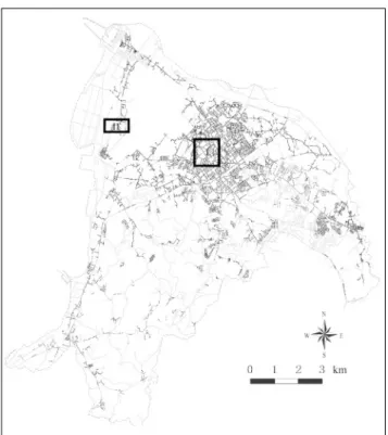
Data for this study came from 1/5000 aerial photo-graphs and GIS data of the study area. ArcView 3.010 _was used to process demand points and location data. As in the research by Valeo et al.,8 _{residential buildings were} regarded as demand points (MSW generation points). Candidate service locations were set at all intersections and points at intervals of 20–30 m along roads. Demand points and candidate service locations were marked as il-lustrated in Figures 2 and 3. There were 8759 demand points and 9216 candidate service locations.

The maximum acceptable walking distances for ser-vice were set to be 50, 70, 85, and 100 m, respectively, for each model to examine the effect of varied distance lim-its on the solutions obtained. CPLEX 6.5,11 _an optimiza-tion software package installed on an inexpensive personal computer with a PII-350 CPU, was applied to solve the models for the case study. The following section describes the results obtained and compares the applicability and merits of the different models.

RESULTS AND DISCUSSION

Table 1 summarizes and compares the results obtained by the different models. For the LSC model with a short

maximum acceptable walking distance for service, more locations were required to satisfy all demands. When the maximum acceptable walking distance was set at 50 m, 2891 locations were required, and at 100 m, only 1087 locations were required. Figure 4 presents a sample result for the SSL solution with the maximum acceptable walk-ing distance set at 100 m. In the figure, a link is added from each demand point to its nearest collection point.

For the sake of comparison, the limit on the number of locations (P) in the MSC and SSL models was set at the number obtained from the LSC model. As shown in Table 1, the average walking distance from demand points to collection locations increased as the maximum accept-able distance increased. The average distance increased from 31–32 m for the maximum acceptable distance of 50 m to 53–58 m for the maximum acceptable distance of 100 m. The sum of total walking distances also increased from 276–287 km to 469–511 km. The average distance and sum of the total walking distances obtained from the LSC and MCL models were similar, whereas the proposed SSL model produced better results. When the maximum acceptable walking distance was 50 m, the average walk-ing distance of the SSL model was ~1.3 m less than those of the other two models, while the sum of total walking distances was 11–12 km less. This difference increased as the maximum acceptable walking distance for service was increased. At the maximum acceptable walking distance of 100 m, the average walking distance of the SSL solu-tion was reduced by 4.8 m, and its sum of total walking distances was reduced by ~42 km in comparison with the

Figure 2. Demand points in the study area.

Figure 3. Candidate collection points in the study area.

other two models. The standard deviation of the results obtained from the SSL model was also lower, except when the maximum acceptable distance for service was 50 m, in which case the standard deviations of all three models were comparable.

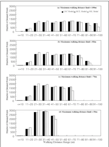
Figure 5 reveals the distribution of demand points under different ranges of walking distances. The SSL model chose service locations closer to demand points than did the other two models. For example, at the maximum ac-ceptable walking distance of 100 m, the SSL solution in-cluded 700 more demand points within 60 m of the walking distance for service than did the LSC and MCL

models. Similar re-sults were observed when the maxi-mum walking dis-tance was set at 50, 70, or 85 m. Figure 6 illustrates the distribution of the number of de-mand points served by collection loca-tions as selected by the different mod-els. At the maxi-mum acceptable walking distance of 100 m, the SSL solu-tion had 657 loca-tions to serve more than 10 demand points, as compared with 594 locations in the MCL model and 388 locations in the LSC model. The SSL solution had fewer locations to serve less than five demand points, while LSC and MCL selected more such inefficient locations.

Table 1. Comparison of the results obtained from the LSC, MCL, and SSL models.

Maximum Number of Model Average Total Standard Computational Acceptable Selected Walking Walking Deviation Solution Time Walking Collection Distance (m) Distance (m) (min) Distance (m) Points 100 1087 LSC 58.40 511,483 23.38 37.0 MCL 58.46 512,053 23.30 143.4 SSL 53.62 469,724 22.26 287.5 85 1366 LSC 50.29 440,476 19.41 23.9 MCL 50.34 440,950 19.36 74.9 SSL 46.73 409,328 18.68 101.3 70 1761 LSC 42.91 375,847 15.31 8.3 MCL 43.14 377,905 15.35 37.8 SSL 40.70 356,493 14.93 55.0 50 2891 LSC 32.81 287,394 9.48 1.7 MCL 32.90 288,168 9.50 11.1 SSL 31.56 276,422 9.49 12.3

Figure 4. The SSL solution with the maximum acceptable walking

distance set at 100 m.

Figure 5. Distribution of collection points in various walking distance

ranges for solutions with maximum walking distance limits of (a) 100 m, (b) 85 m, (c) 70 m, and (d) 50 m.

Kao and Lin

Similar results were obtained at the maximum acceptable walking distances of 50, 70, and 85 m. The SSL solution had a shorter average walking distance and more loca-tions able to serve more demand points. This result im-plies that a pickup truck can stay longer at a location, thereby increasing the efficiency of the collection service. Table 1 also compares the computational time for solving different models. The solution time was lowest at the maximum acceptable walking distance of 50 m for all models, because the fewest locations are required to sat-isfy the maximum walking distance constraint. As the maximum acceptable walking distance was increased, the solution time increased. When the distance doubled from 50 to 100 m, the solution time increased 12–22 times. The LSC model took the least computational time, while the SSL model required 8 times as much time because it involves more variables. However, the rapid advancement of computer technology enables a large real-world prob-lem to be solved within an acceptable computational time with a relatively inexpensive personal computer.

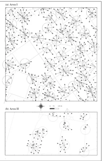
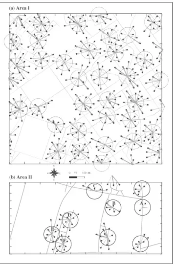
Solutions for two regions, indicated as I and II in Fig-ure 2, were magnified for solutions with the maximum acceptable walking distance of 100 m for ease in visualiz-ing the differences among results and the efficiency of

the recommended SSL model. The results obtained from the three models for both regions are shown in Figures 7–9, respectively. The circles in the figures were drawn with the collection location as the center and the average walk-ing distance, based on the SSL solution (53.62 m), as the radius to facilitate the comparison of service areas. In Fig-ures 7a and 8a, collection locations were randomly se-lected in the LSC and MCL models when they fell within overlapping covered service areas. These randomly se-lected points may result in longer walking distances for demand points. The SSL solution included fewer locations with overlapping service areas.

Figures 7b–9b magnify a more independent region to easily demonstrate the difference. In area A, there are two demand points. The LSC and MCL models randomly selected a poor location within the maximum acceptable walking distance to serve these two demand points, thereby increasing their walking distances as compared with the SSL solution. The resulting walking distance from one of the points to the service location was longer than the average walking distance, indicated by the correspond-ing circle. The SSL model selected the location with the

Figure 6. Distribution of demand points served by all collection points

for solutions with maximum walking distance limits of (a) 100 m, (b) 85 m, (c) 70 m, and (d) 50 m.

Figure 7. The LSC solution: (a) Area I and (b) Area II.

shortest sum of walking distances for the two demand points and was thus able to choose the best location. Such a prob-lem involving only two demand points is easily recognized and rectified during real collection. But the following situa-tions cannot be rectified so easily. In the same figures, areas B and C include a total of 10 demand points. The SSL model selected better locations than did the other models in that only two of the 10 points fell outside the average walking distance. In both the LSC and MCL solutions, four demand points fell outside the average walking distance. Similar situ-ations occurred in areas D, E, and F, in which the LSC and MCL solutions had five more points falling outside the av-erage walking distance than did the SSL solution. Area D in the LSC and MCL models serves only two and three de-mand points, respectively. In area F, the LSC and MCL solu-tions can serve 15 demand points, more than those served by the location selected in the SSL solution, but 11 of them fell outside the average walking distance, resulting in poorer service. As demand and the number of collection locations increases, manually rectifying the results derived from the LSC and MCL models is more difficult, thereby making it worthwhile to apply the SSL model to more efficiently se-lect a proper colse-lection location set.

CONCLUSION

Selecting the locations of an appropriate number of pickup locations before the implementation of an MSW pickup system is important to the cost efficiency and service quality of the system. This study employed the LSC, MCL, and SSL models to determine collection lo-cations. All three models found solutions within an ac-ceptable computational time using a low-end personal computer. The SSL model, although taking longer to obtain solutions, produced more efficient results, short-ening the service walking distance and thus enhancing the quality of service. This study also compared the ef-fect of varied maximum acceptable walking distance limits for service. More locations are required if the maximum acceptable walking distance is shorter, result-ing in increased cost and collection time. Conversely, a long maximum acceptable walking distance limit re-sults in fewer locations and a lower cost but less cus-tomer satisfaction because of longer walks to drop MSW. The optimal walking distance for the service should be determined according to affordable collection cost, de-sired collection time, and service quality expected by the general public.

Figure 8. The MCL solution: (a) Area I and (b) Area II. Figure 9. The SSL solution: (a) Area I and (b) Area II.

Kao and Lin

Certainly, the possibility always exists to improve this model. The real-world implementation of the pickup sys-tem is not exactly the same as the solution herein be-cause of special requests from local residents, unusual road conditions, traffic limitations, and so on. These issues were not included in the model and, in the future, may be ex-plored further by an enhanced model or some other ap-proaches such as a multicriteria analysis, as suggested by an anonymous referee.

ACKNOWLEDGMENTS

The authors thank the Bureau of Environmental Protec-tion of the Hsinchu Municipal Government for provid-ing data for the case study. Dr. H.Y. Lin is also commended for his valuable discussions of the SSL model.

REFERENCES

1. Toregas, C.; ReVelle, C. Optimal Location under Time or Distance Constraints; Papers Regional Sci. Assoc. 1972, 28, 133-143.

2. Church, R.; ReVelle, C. The Maximal Covering Location Problem; Papers Regional Sci. Assoc. 1974, 32, 101-118.

3. ReVelle, C.; Hogan, K. The Maximum Availability Location Problem; Transport. Sci. 1989, 23 (3), 192-200.

4. Rose, G.; Bennett, D.W.; Evans, A.T. Locating and Sizing Road Main-tenance Depots; Eur. J. Operat. Research 1992, 63, 151-163. 5. Swersey, A.J.; Thakur, L.S. An Integer Programming Model for Locating

Vehicle Emissions Testing Stations; Manage. Sci. 1995, 41 (3), 496-512. 6. Church, R.L.; Stoms, D.M.; Davis, F.W. Reserve Selection as a

Maxi-mal Covering Location Problem; Biolog. Conserv. 1996, 76, 105-112.

7. Downs, B.T.; Camn, J.D. An Exact Algorithm for the Maximal Cover-ing Problem; Naval Research Logist. 1996, 43, 435-461.

8. Valeo, C.; Baetz, B.W.; Tsanis, I.K. Location of Recycling Depots with GIS; ASCE J. Urban Plan. Devel. 1998, 124 (2), 93-99.

9. Siddiqui, M.Z.; Everett, J.W.; Vieux, B.E. Landfill Siting Using Geo-graphic Information Systems: A Demonstration; ASCE J. Environ. Eng. 1996, 122 (6), 515-523.

10. Using ArcView GIS; Environmental Systems Research Institute: Redlands, CA, 1996.

11. CPLEX 6.5 User’s Manual; ILOG S.A.: Gentilly Cedex, France, 1999.

About the Authors

Jehng-Jung Kao (corresponding author) is currently a pro-fessor at the Insititute of Environmental Engineering, Na-tional Chiao Tung University, 75 Po-Ai St., Hsinchu, Taiwan, Republic of China; e-mail: jjkao@ensys.ev.nctu.edu.tw. At the time this work was conducted, Tsung-I Lin was a gradu-ate student in the Institute of Environmental Engineering, National Chiao Tung University. At present, he is working as an engineer at the Axtronics Information Appliances Inno-vator Co., Taiwan, Republic of China.