RuO2和IrO2的電子傳輸性質

國

立

交

通

大

學

電子物理系

碩

士

論

文

RuO

和 IrO

的電子傳輸性質

Electronic transport properties in RuO

and IrO

nanowires

研 究 生：包智傑

指導教授：陳煜璋 教授

RuO

和 IrO

的電子傳輸性質

Electronic transport properties in RuO

and IrO

nanowires

研

究 生：包智傑 Student：Jhih-Jie Bao

指導教授：陳煜璋

Advisor：Yu-Chang Chen

國

立 交 通 大 學

電

子 物 理 系

碩

士 論 文

Submitted to Department of Electrophysics College of Science

National Chiao Tung University in partial Fulfillment of the Requirements

for the Degree of Doctor of Philosophy

in Electrophysics

July 2009

Hsinchu, Taiwan, Republic of China

RuO

和 IrO

的電子傳輸性質

學生：包智傑

指導教授

陳煜璋

國立交通大學電子物理學系﹙研究所﹚碩士班

摘要

Electronic transport properties in RuO

and IrO

nanowires

學生：Jhih-Jie Bao

指導教授

Yu-Chang Chen

Department﹙Institute﹚of Electrophysics

National Chiao Tung University

Abstract

RuO and IrO₂ are the inviting electrical contact materials which exhibit the metallic conductivity properties at room temperatures. They crystallize in the rutile structures and display good thermal stability at high temperatures. We study the size effects of the transport properties of RuO2 and IrO2 nanowires using

first-principles approaches. The relaxed structures of RuO2and IrO2 bulk and

nanowires are obtained based on the density functional theory. By using the force tensor we calculate the phonon dispersion relation of the RuO2 and IrO2

nanowires with different diameters. We observe that the sound velocities and the Debye temperatures display size effects. According to the Bloch-Gruneisen model within Matthiessen’s rule, the resistivity varies as 5

T at low temperatures due to electron-phonon interactions. At the same temperatures, the size effects of the sound velocity and the Debye temperatures lead to the increase of the resistivity as the diameters of the nanowires increase.

致謝

Contents

2-3 Density Functional Theory ... 7

2-3-1 Hohenberg and Kohn theorem11 ... 7

2-3-2 Kohn-Sham equation12... 9

(A) Pseudopotential Method ... 10

(B) Pseudopotential15 ... 12

(C) Local Density Functional Approximation ... 14

2-4 Band Theory ... 16

2-5 Phonon dispersion relation ... 18

2-5-1 Two atoms per primitive basis21 ... 18

2-5-2 Acoustic and optical phonon ... 20

2-5-3 Debye model for density of states ... 21

2-5-4 Phonon dispersion relation22-24 ... 22

2-5-5 Calculation of the force constant matrix ... 22

Chapter3 Calculation Method and Result ... 25

3-1 Crystal structures ... 25

3-2 VASP Calculation ... 30

3-3 Phonon dispersion relation ... 32

3-4 Matthiessen’s rule25 _{... 37}

3-5 Results and Discussion ... 40

3-5-1 Debye temperature calculation27, 28 ... 40

3-5-2 Bloch-Gruneisen Model calculation ... 42

Chapter4 Conclusion ... 44

List of Figures

Fig. 1.1 The heat capacity of IrO2 and RuO2

3_{. ... 2}

Fig. 1.2 Resistivity versus temperature of IrO2 and RuO2 4_{. ... 2}

Fig. 1.3 The resistance as a function of temperature for different diameter in 2 RuO and IrO₂5. ... 3

Fig. 3.1 The primitive cells for RuO2(upper panel) and IrO2 (lower panel) in the rutile structures. ... 27

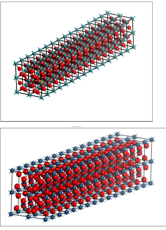
Fig. 3.2 The structure of 1x1 nanowire for RuO2 (upper panel) and IrO2(lower panel). The picture of the top-left corner is its bulk structure. ... 28

Fig. 3.3 The structure of 2x2 nanowire for RuO2 (upper panel) and IrO2(lower panel). ... 29

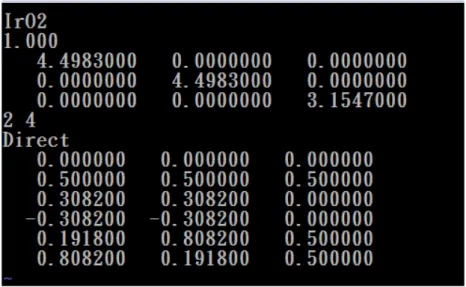
Fig. 3.4 The contents of the POSCAR file. ... 30

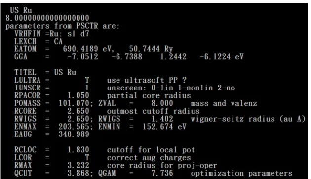
Fig. 3.5 The partial contents of POTCAR file for local-density approximation. ... 31

Fig. 3.6 The contents of the KPOINTS file. ... 31

Fig. 3.7 The contents of the INCAR file. ... 32

Fig. 3.8 All output files of the VASP. ... 32

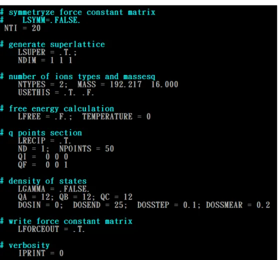
Fig. 3.9 The contents of the INPHON file. ... 33

Fig. 3.10 The contents of the DISP file. ... 34

Fig. 3.11 The contents of the FORCES file. ... 35

Fig. 3.12 Phonon dispersion relation for the RuO2(upper panel) and IrO2(lower panel). ... 36

Fig. 3.13 The dependence of the Debye temperature in RuO2 (upper panel) and 2 IrO (lower panel) on the diameters of the nanowires. ... 41

Fig. 3.14 The resistivity of RuO2 (upper panel) and IrO2 (lower panel) nanowires due to the interactions between electrons and the acoustic phonons. ... 43

Chapter1 Introduction

The rutile-structure transition-metal dioxides exhibit a variety of interesting physical properties that RuO2 and IrO2 have good conductivity properties and

stability at high temperature. Their electrical transport properties are investigated for a long time, both experimentally and theoretically.

The electronic structures of RuO2 and IrO2 have been studied using the

self-consistent semirelativistic linear muffin-tin-orbital (LMTO) method associated with the atomic sphere approximation in 1989 by J. H. Xu, T. Jarlborg and A. J. Freeman1. Their results are in good agreement with experiments. In 1993, Keith M. Glassford and James R. Chelikowsky2 have calculated the structures and electronic properties of

2

RuO using ab initio density functional theory with a fast iterative diagonalization technique with local-density-approximation (LDA) in a plane-wave basis and the pseudopotential.

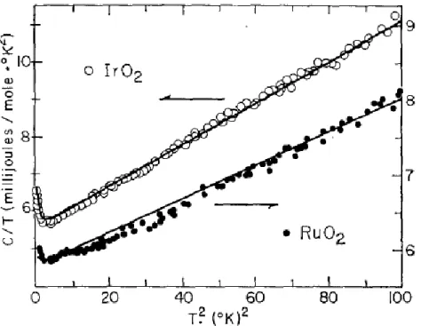
In experiments, the heat capacities of RuO2 and IrO have been measured in 2

1969 by B. C. Passenheim and D. C. McCollum3. The heat-capacity measurements have been made by discontinuous heating method in a He cryostat. Their results show

that 2 3

0.059 0.0225 5.77

C= T− + T + T ( mJ mole K/ ⋅ ) for RuO2 , and

2 3

0.308 0.0565 5.51

C= T− + T + T (mJ mole K/ ⋅ ) for IrO2. The experiment data is

Fig. 1.1 The heat capacity of IrO2 and RuO2

3_.

W. D. Ryden and A. W. Lawson4 have measured the resistivity of RuO2 and IrO2

in the temperature range 4.2-1000 K in 1970. They have found the relation based on electron-electron and electron-phonon interband scatterings and fitted the temperature dependence of the resistivity. The figure 1.2 is the result of their experiment.

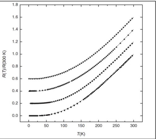
In 2004, J. J. Lin, S M Huang, Y H Lin, H Liu, X X Zhang, R S Chen and Y S Huang5, 6 firstly report their measurements of the resistivities and magnetoresistivities of RuO2 and

2

IrO nanowires over a wide temperature range from 300 K down to 0.3 K .

Prof. Juhn-Jong Lin’s group employs a thermal evaporation method to synthesize

2

RuO nanowires with controlled sizes. They control the sizes of the RuO₂ nanowires by adjusting the growth time and the average width of nanowires is about ~ 90nm . When they measure the transport properties of different diameters of nanowires, they find that the conductivities of the thick nanowires are better than the thin ones7. The results agree well with our ideal conjecture and we get the same relation in the theoretical calculation. In the figure 1.3, the resistivity varies with the temperature and they shift a constant in different diameters. The argument is similar for our results.

Fig. 1.3 The resistance as a function of temperature for different diameter in RuO2

and IrO2

5_.

Motivated by the above experiments, we theoretically investigate the dependence of the resistivity on the diameters of RuO2 and IrO2 nanowires in this

work. We have calculated the Debye temperature of different diameters and compared the theoretical results with the experiments performed by Prof. Juhn-Jong Lin’s group. We use Vienna Ab-initio Simulation Package (VASP)8 to relax the structures and the force constants of RuO and IrO bulk and nanowires. We also investigate the

phonon dispersion relation for RuO2 and IrO2 nanowires with different diameters,

and the size effects on the electron transport according to the Bloch-Gruneisen equation.

The outline of the thesis is described as followings: first, we introduce the theories which we have applied to calculate the Debye temperature and resistivity in chapter 2. In section 2-1, we introduce the Hartree approximation; in section 2-2, we introduce the Hartree-Fork approximation; in section 2-3, we introduce the density functional theory (DFT); in section 2-4, we introduce the band theory; and in section 2-5, we introduce the phonon dispersion relation.

In chapter 3, we introduce the structures of RuO2 and IrO2 nanowires and

the bulk crystals. We explained the parameters of VASP that is used to relax the structures of our systems. We also explain how to use “PHON”9 to obtain the phonon dispersion relations and the sound velocities. We also present the results of our calculations and discussion in the later part of the third chapter. According to the Matthiessen’s rule with electron-phonon scatterings, we find the relation between the resistivity in the Bloch-Gruneisen model and the temperatures. We also study the relation of the Debye temperature versus diameters nanowires. Our objective is to theoretically investigate the trend of the conductivities and Debye temperatures as the function of the diameters of nanowires.

Chapter2 Theories

In this chapter we briefly introduce the theories of density functional theory and the theories of phonons. We introduce the Hartree and Hartree-Fock approximations in sections 2-1 and 2-2. In section 2-3, we introduce the density functional theory (DFT), which the ground state properties of a many electron system are uniquely determined by the electron density n r( ). In section 2-3-1, we introduce the Hohenberg and Kohn

theorem. In section 2-3-2, we introduce the local density functional approximation (LDA) and the scheme of self-consistent calculations. In section 2-4, we briefly introduce the Bloch theorem and the band theory. In the section 2-5, we introduce the phonon dispersion relation and the phonon frequency from calculation the force constant matrices.

In many-electron system, the potential energies of electrons are complicated and the wave functions of many-electron system are difficult to solve. Density functional theory can simplify the calculations by mapping the complicated many-body wave functions into effective single-particle wave functions, where the effects of weak electron-electron interactions are included in the exchange-correlation energy.

2-1 Hartree approximation

Consider the Hamiltonian of many-particle system with N electrons can be written as 2 2 1 , 2 2 N N N i ext i i j _{i j} p e H V m r r = + + −

∑

∑∑

In the absence of the interaction between electrons, the many-body system will decouple into one-body problems. The ground-state wave function of the many-body system is expressed as the simple product of orthonormalized one-electron wave functions.

1 2 1 1 2 2

( , ,r r ,r_N) ψ ( )r ψ ( )r ψ_N(r_N).

Ψ ⋅⋅⋅⋅⋅ = ⋅⋅⋅⋅⋅ (2.2) The total energy of the system is given by E= Ψ H Ψ . By using the variational

constraint ψ ψi j =δij , the effective single-particle Schrodinger equation can be expressed as 2 , 2 ext H l l l p V V m ψ ε ψ  _{+ +}  ₌     (2.3) where _ext 2 . R _i Ze V r R = − −

∑



of the ions in the potential field Vext in the Coulomb potential of an average distribution of all other

electrons. _{3 '} 2 ' ' ( ) H j e V d r n r r r = −

∫

electron-electron interactions. j( ) j( )2

j

n r =

∑

The Eq.(2.3) is also called Hartree equation, and one can use the pseudopotential method to approximate the potential Vext and the potential VH.

2-2 Hartree-Fock approximation

Because the electrons are fermions, the total wave function is antisymmetric. To satisfy the Pauli Exclusion principle, one can extend the expression Eq.(2.2) as the Slater determinant of single particle wave functions:

1 1 1 1 2 2 1 2 1 1 2 2 2 1 1 ( , ) ( , ) ( , ) ( , ) ( , ) 1 , ! ( , ) ( , ) N N N N N N r s r s r s r s r s N r s r s ψ ψ ψ ψ ψ ψ ψ Ψ =          (2.4)

where s denotes the electron spin.

By using the variational principle with the constraint ψ ψi j =δij, Eq.(2.3) can be

2 . 2 ext H x l l l p V V V m ψ ε ψ   + + + =     (2.5)

We see that Eq.(2.5) has one more term than Eq.(2.3) on left-hand side of the equal sign which is called exchange potential _{3 ' *} ' 2

' ( ) ( ) x i j j i e V d r r r r r ψ ψ ≠ = − −

∑

The exchange potential Vx has the relations with Pauli Exclusion Principle and is

a nonlocal potential. It can be calculated by using the local density functional approximation.

2-3 Density Functional Theory

The fundamental physical quantities in the ground state can be uniquely described from the electron density ( )n r in many-particle system. All ground state properties of the many electron system are functional of ( )n r . In 1964 Hohenberg and Kohn prove that the ground state electron density uniquely determines the external potential. Kohn and Sham extended the theorem by separating the total energy into the kinetic energy of electron, the potential energy of attraction between electrons and nuclei, the coulomb potential energy of repulsion, and the exchange-correlation energy between electrons.

2-3-1 Hohenberg and Kohn theorem

The external potential is uniquely determined by the ground state electron density. The above theorem can be proved as follows：

We assume that two different potential V and 1 V2 have the same ( )n r

 .

Suppose V1≠V2+constant and Ψ ≠ Ψ where 1 2 Ψ is the ground state wave 1

function. The Schrodinger equation can be expressed as

1 1 1 1

2 2 2 2,

H Ψ = Ψ E

where E1 and E2 are eigen-energies of H1 and H2, respectively.

With different external potentials, the Hamiltonian can be expressed as

1 2 1 2.

H =H + −V V

Because E1= Ψ1 H1 Ψ1 is the ground energy, we can obtain

1 H1 1 2 H1 2 Ψ Ψ < Ψ Ψ 3 1 2 2 2 2 1 2 2 2 ( 1 2) ( ), E < Ψ H Ψ + Ψ V −V Ψ =E +

∫

∫

3

1 2 ( 1 2) ( ) 1 2,

E −E <

∫

(2.8)

which leads to a contradiction and means that the assumptions are wrong. Thus, two different external potentials cannot correspond to the same non-degenerate ground state density. The total energy can be expressed as a functional of ground state charge density ( )n r in many-electron system.

[ ].

tot T

E =E n

If the charge density ( )n r is determined, all the ground state properties of the many-electron system will be determined.

2-3-2 Kohn-Sham equation

From the Hohenberg and Kohn theorem, it is known that the ground state properties of many-particle system can be determined by the electron density ( )n r . The charge density in the ground state can be solved iteratively until the self-consistent is achieved.

The ground state energy of a homogeneous interacting electron gas can be written as ' 3 3 3 ' ' 1 ( ) ( ) [ ] [ ] ( ) ( ) [ ]. 2 T ext xc n r n r E n T n V r n r d r d rd r E n r r = + + + −

∫

∫∫

In the right-hand side, the first term is the kinetic energy as a functional of non-interacting electrons with density ( )n r ; the second term is external potential energy relative to electrons; the third term is Coulomb energy between electrons; and the fourth term is the exchange-correlation energy functional of an interacting system with density ( )n r . By the variational principle with the total electron N =

∫

3 ' [ ] ( ) ( ) ( ) , ext xc T n n r V r d r V r n _{r r} δ _µ δ + +

∫

∫

In the absence of the exchange-correlation potential, it goes back to Hartree approximation. Comparing Eq.(2.10) with Eq.(2.5), it is regarded as an effective potential of the single-electron wave equation which is called Kohn-Sham Equation.

2 2 ( ) ( ) ( ) ( ) ( ), 2m Vext r VH r Vxc r ψi r ε ψi i r   − ∇ + + + =           _(2.11)

[ ]

xc

E n is the exchange and correlation energy of an interacting system with density ( )n r .

(A) Pseudopotential Method

The early calculations of first-principles pseudopotential are made within the scheme of orthogonalized-plane-wave (OPW) atomic calculation. The wave functions in this way exhibit the correct shape outside the core region; however, they differ from the real wave functions by a normalization factor13. Hamann, Schluter and Chiang14 (HSC) propose a model pseudopotential to solve the problems that have four properties：(1) real and pseudo valence eigenvalues agree for a chosen atomic configuration; (2) real and pseudo wave functions agree beyond a chosen core radius

c

r ; (3) the integrals from 0 to r of the real and pseudo charge densities agree for r> r_c for each valence state, this is norm conservation condition; (4) The logarithmic derivatives of the real and pseudo wave function and their first energy derivates agree for r> . rc

Because the lattice has the periodic characteristic, the wave functions must satisfy the Bloch theorem. It can be written as expansion of the following form:

( ) 1 ( ) nk i k G r. nk G G r α e + ⋅ Ψ = Ω

∑

In the pseudopotential method, the pseudopotential Vps is constructed on the

valence electrons and the core electrons have been transformed away. The pseudo-Hamiltonian of the valence electrons can be expressed as

2 , 2 ps H xc p H V V V m = + + + (2.13) where ( ). ps ion j R V =

∑

angular momentums of the electron in the s, p and d orbitals are 0, 1 and 2, respectively. The potential can be expressed as

 2 0 ( ) ( ) . ion l l i V r V r P = =

∑

P is the projection operator of the angular momentum . The Hartree potential satisfies the Poisson equation and it can be written as

2 ( ) 8 ( ). H V r πn r ∇  = −  (2.15) ( )

n r _{is the density of the pseudo valence electrons and the} V_xc can be regarded as functional of ( )n r from LDA. We define the elements of the matrix Sthat

' ' ' , , . k G G G G S  = k   +G k+G =δ  (2.16)

The pseudopotentials of the ion Vion can be separated into local and non-local

potential ( loc nl

ion ion ion

V =V +V ). The V_H and V_xc are functional of ( )n r that are also local potential. The Hamiltonian can be rewritten as

loc nl H = +T V +V 2 , 2 p T m = (2.17) ' 2 ' , , G G k +G T k +G = +k G δ  (2.18) ' ' ( ), loc loc k +G V k +G =V G G − (2.19) ' ' ( , ). nl nl k +G V k +G =V k   +G k+G (2.20)

(B) Pseudopotential

Pseudopotentials are introduced to simplify electronic structure calculations by eliminating the need to atomic core states and the strong potentials responsible for binding them.

To construct atomic pseudopotential ϕlm at a given energy which are identical to

atomic eigenfunctions. The ϕlm are continued inside rc with the condition that l

lm r

ϕ → for r→0 and with the norm-conserving condition, one has

2 3 2 3 0 0 , c c r r lmd r lmd r ϕ = ψ

∫

∫

The pseudopotentials are obtained by inverting the Schrodinger equation

2 2 ( 1) ( ) [ ] / . l r l l l l V r E r ϕ ϕ + = ∇ + − (2.22)

The complete pseudopotential is then written as

( ) ( ) ( ) ,

PS loc non loc lm l lm

lm

V =V +V =V r +

∑

where δυ_l = for 0 r> and r_c V_loc is the local potential and is an arbitrary function for r< . The semilocal formrc

16 _{(i.e. nonlocal in angular coordinates but local in radial}

coordinate) of the Hamman-Schluter-Chiang (HSC) pseudopotential which used in an expansion of N plane waves requires the evaluation of ( 1)

2 N N +

integral for each

l

δυ . The nonlocal form can be introduced,

1 ( ) ( ) ( ) ( ) , ps loc lm l l lm l lm V =V +

∑

the ,lm and also includes two or more energies at which the ϕ_lm( )r are evaluated. This result in Bl becoming a matrix

,

ij i j j

B = ϕ δυ ϕ

which is not Hermitian and the generalized norm-conservation requirement,

3 * * 3 0 ( ) 0 ( ) ( ) ( ) ( ) 0, c c r r ij ij i j i j Q =

∫

∫

and Vanderbilt17 _defines

1 ( ) , i ji j j j B β ₌

∑

which is substituted into the Eq.(2.24) and one can obtain the pseudopotential

,

.

ps loc i ij j

i j

V =V +

∑

In general, it is difficult to apply Eq.(2.25), results in ϕlm whose plane-wave

expansions are extremely slowly converging. To avoid applying Eq.(2.25), Chou18 constructed norm-conserving ϕ at two energies nlm En and inverted the Schrodinger

equation to obtain their δυnl which she averaged to obtain δυ , yielding l

1 ( ) _rlm( ) l( ) _rlm( ) l( ) , ps loc nl nlm V =V r +

∑

The Anl is Hermitian and the ϕnlm( )r are solutions of the pseudo Schrodinger

(C) Local Density Functional Approximation

The exchange-correlation energy is relation to the electronic distribution in the system. It is difficult to give an exact expression for Exc because of its complexity. In

order to simplify this complexity, Kohn and Sham suggested using the homogeneous electron gas system to approximate the energy contribution from E_xc[ ]n in 1965. If the electronic density varies slowly, the exchange-correlation functional can be written as 3 [ ] [ ] ( ) , xc xc E n =

∫

where the exchange-correlation potential can be expressed as [ ] ( ) xc { ( )}, xc xc E n d V r n n n dn δ _ε δ = =  (2.30)

where ε_xc[ ]n is the exchange-correlation energy density of the homogeneous electron gas. V_xc( )n is the exchange and correlation contribution to the chemical potential of a homogeneous gas of density n .

The exchange-correlation energy density19 can be separated into ε_x[( )]n and

[( )]

c n

ε  . ε_x[( )]n is the exchange energy of a homogeneous electron gas and ε_c[( )]n

is the correlation energy of a homogenous electron gas.

Within Hartree-Fock approximation the exchange energy density can be obtained by solving the Schrodinger equation of the non-interacting homogenous electron gas.

0.458 ( ) x s r r ε  =− rs is Wigner-Seitz radius, where 1 3 1 3 4 4 ( ) ( ) ( ) 0.458( ( )) . 3 s x 3 n r = πr − ⇒ε r = − πn r (2.31) From the Eq.(2.31), we can know that the exchange energy density ε_x( )r is

An approximation of the correlation energy is based on Quantum Monte Carlo calculations by Ceperley and Alder20. The wave function for electrons in a finite volume subject to periodic boundary conditions and extrapolated the energy per electron to infinite volume. The Ceperley’s parameterization of the correlation energy for r_s ≥ is 1

1 2 0.1423 ( ) , 1 1 1.0529 0.3334 s c s s s s r r r r r r ε β β − = = + + + +  (2.32)

the high-density form of εc (rs < ) is 1

( ) 0.0311ln 0.048 0.002 ln 0.0116

c r rs rs rs rs

ε  = − + −

Substituting Eq.(2.31) into Eq.(2.30), the relation between exchange-correlation potential and electronic density can be expressed as

[1 ] . 3 s xc xc s r d V dr ε = − (2.33)

In many-electron system, we give the initial data of the electronic density to calculate the potential each term, and get the effective potential Veff to solve the

solution of the Kohn-Sham equation. The wave function is obtained by Kohn-Sham equation and the new electronic density is calculated from the wave function. If the difference in value between the new electronic density and the initial electronic density is too big, they will be mixed to generate another electronic density, and repeat the above procedures until the difference in value between the new density and last density is very small. The above procedures are called self-consistent procedure.

The convergence of the flow chart：

KS equation

;

1

(1

)

V

solve

_out

converngence

in

eff

i

i

n

n

n

out

in

in

ρ

ε ψ

ρ

ρ

α ρ

αρ

→

→

→

→

→

+

↑ ← ←

= −

+

← ← ↵

2-4 Band Theory

The solutions of the Schrodinger equation for a periodic potential by Bloch theorem can be expressed as

( ) i k r ( ),

k r e u rk

ψ  ₌  ⋅  _(2.34)

where u r_k( ) has the period of the crystal lattice with u r_k( ) =u r_k( +R). We substitute Eq.(2.34) into the Kohn-Sham equation

2 2 ( ) ( ) ( ) ( ) ( ), 2m Vext r VH r Vxc r ψk r ε ψk k r   − ∇ + + + =            _(2.35) here 2 2 2 2 2 2 ( ) [ ( )] [ ( ( ))] 2 2 2 [ ] ( ), 2 i k r i k r k k k k i k r k r e u r e iku u r m m m e ik u r m ψ ⋅ ⋅ ⋅ − ∇ = − ∇ ∇ = − ∇ + ∇ = − + ∇                      

The Kohn-Sham equation is rewritten as

( ) ( ), k k k k H u r =ε u r where 2 2 [ ] ( ) ( ) ( ). 2 k ext H xc H ik V r V r V r m = −   + ∇ +  +  + 

This is a partial differential equation with complicate boundary condition. One can reduce this complicate boundary value problem to a simple matrix diagonalization problem using Rayleigh-Ritz variational principle.

We choose a basis function χ_n( ),r

and _k( ) _{n n}( ).

n

u r =

∑

According to the variational principle, we know that the expectation value of the Hamiltonian by the arbitrary wave function must be greater than ground-state energy of the system. , k k GS u H u ≥E or 0. k k GS k k u H u −E u u ≥ (2.37)

If one can find out the minimum eigenvalue of the system, one will get the energy close to the ground-state energy. We substitute Eq.(2.36) into Eq.(2.37) with the equal sign the variational principle tell us that in the ground state

* n n k m m * n n m m 0, n m n m l l C H C C C C χ χ λ C χ χ ∂ ₋ ∂ ₌ ∂

∑

∑

∑

∑

∑∑

∑∑

More compactly one may write in this way.

( ) 0 lm m lm m m m H k C −λ S C =

∑

∑

If the matrices Hnmand Snm are given, the wave functions can be obtained by

LPAW, LCAO, etc.

2-5 Phonon dispersion relation

A phonon is a quantized mode of vibration occurring in a rigid crystal lattice.

2-5-1 Two atoms per primitive basis

Consider the elastic vibrations of a crystal which is correlated to displacements of other atoms nearby. Most simple situation is obtained in the [100], [110] and [111] propagation directions of cubic crystals. If a wave is propagating along one of these directions entire planes of atoms move in phase with displacements either parallel (longitudinal) or perpendicular (transverse) to the direction of the wave vector K.

Here we think about two different atoms per primitive basis. Atom 1 with mass

1

M is displaced by u_s−1,u u_s, _s+1 and atom 2 with mass M₂ is displaced by

1, , 1

s s s

υ υ υ_{− +} , where M1>M2. The force constant is C and force between two

different neighboring atoms is F =C(υ_s−u_s) from Hooke’s law. The equation of motion is 2 1 2 1 2 2 2 1 ( 2 ) ( 2 ). s s s s s s s s d u M C u dt d M C u u dt υ υ υ _υ − + = + − = + − (2.39)

The solution in the form of a traveling wave with different amplitude ,u υ can be written as ( ) ( ) , i sKa t s i sKa t s u ue e ω ω υ υ − − = = (2.40)

where the lattice constant a is defined as between nearest identical planes, not nearest-neighbor planes. Substitute Eq.(2.40) into Eq.(2.39) and we can get

2 1 2 2 (1 ) 2 ( 1) 2 , iKa iKa M u C e Cu M Cu e C ω υ ω υ υ − − = + − − = + − (2.41)

Transform the above equation to another type 2 1 2 2 (2 ) (1 ) 0 ( 1) (2 ) 0, iKa iKa C M u C e C e u C M ω υ ω υ − − − + = − + + − = (2.42)

The solution of the phonon dispersion relation can be found by the determinant of the coefficients of above equation:

2 1 2 2 2 (1 ) det 0, ( 1) 2 iKa iKa C M C e C e C M ω ω − − − + = − + − (2.43) here 4 2 2 1 2 2 ( 1 2) 2 (1 cos ) 0, M M ω − C M +M ω + C − Ka =

and it is known cos 1 ( )2 ( )4 1 ( )2

2! 4! 2! Ka Ka Ka Ka= − + +≈ − when Ka1 2 2 2 2 1 2 1 2 1 2 2 1 2 1 2 1 2 2 1 2 1 2 1 2 1 2 2 ( ) 4 ( ) 4 ( ) 2 2 ( ) {2 ( )[1 ( ) ] } , 2 C M M C M M M M C Ka M M M M C M M C M M Ka M M M M ω = + ± + − + ± + − + = (2.44) then 1/ 2 1 (1 ) 1 2 x x

+ ≈ + when x1 and the above equation is similar

2 1 2 1 2 1 2 2 2 1 2 1 2 ( ) { ( )[1 ( ) ]} 2( ) . M M C M M C M M Ka M M M M ω + ± + − + = (2.45)

We can get the two solutions of the Eq.(2.45).

2 1 2 1 1 2 (C ), M M ω = + (2.46)

2 2 1 2 ( ) , 2( ) C Ka M M ω = + (2.47)

where Eq.(2.46) is called optical branch and Eq.(2.47) is called acoustical branch. For first Brillouin zone the boundary condition is K

a a π π − _< < . At Kmax a π = ± we can get the solution 2 2 2C M

ω = for optical mode

2 1

2C M

ω = for acoustical mode

2-5-2 Acoustic and optical phonon

It is mentioned before that there are two types of phonons: acoustic phonon and optical phonon in solid with more than one atom in the smallest unit cell.

The acoustic phonons which are the phonons described above and have frequencies that become small at the long wavelengths, and correspond to sound waves in the lattice.

The optical phonons, which also arise in crystals with more than one atom in the smallest unit cell, always have some minimum frequency of vibration, even when their wavelength is large. They are called optical because in ionic crystals (like sodium chloride) they can be excited by light (in fact, infrared radiation). Optical phonons that interact in this way with light are called infrared active. Optical modes correspond to a vibration where the positive and negative ions at adjacent lattice sites swing against each other, creating a time-varying electrical dipole moment.

If there are p atoms in the primitive cell, there are 3p branches to the dispersion relation：3 acoustical branches and 3p− optical branches. For example, 3 germanium have two atoms in the primitive cell, have six branches ： one LA (longitudinal acoustical) , one LO (longitudinal optical) , two TA (transverse acoustical) and two LA (longitudinal acoustic).

accounting for 3N of the total degrees of freedom. The remaining (3p−3)N degrees of freedom are accommodated by the optical branches.

2-5-3 Debye model for density of states

We apply periodic boundary conditions over 3

N primitive cells and consider a cube with length L . The total number of states in K space with the volume of a sphere of radius K ： 3 3 4 ( ) ( ) 2 3 L K N π π = (2.48)

The density of state for each polarization is

2 2 ( ) ( )( ) 2 dN VK dK D d d ω ω π ω = = (2.49)

In the Debye approximation the dispersion relation is written as

K

ω υ= (2.50)

where υ is the velocity of the sound. Substitution Eq.(2.50) into Eq.(2.49), the density of states becomes 2 2 3 ( ) 2 V D ω ω π υ = (2.51)

A cutoff frequency ωD is determined by Eq.(2.49) as

3 3 3 2 3 6 D KD N V ω υ π υ = = (2.52)

The Debye temperature Θ in terms of D ωD is defined as

1 2 3 6 ( ) D D B B N k k V ω υ π Θ ≡ =  ⋅ (2.53)

2-5-4 Phonon dispersion relation

We apply the code “PHON” to calculate the force constant matrices and phonon frequency in crystals. “PHON” is an open source code, developed by Dario Alfe. The phonon dispersion relations have been calculated using ab-initio force constant method using the VASP program.

The central quantity in the calculations of the phonon frequencies is the force-constant matrix Φisα β,jt . The force constant matrices are calculated in terms of

Hellmann-Feynman forces by the displacement of a single atom in the frame work of self-consistent density functional theory calculations in the local density approximation.

The frequencies at wave vector k are the eigenvalues of the dynamical matrix

, s t D_{α β}, defined as ( ) , , 1 ( ) ik Rjt Ris , s t is jt i s t D k e M M α β α β ⋅ − =

∑

where the atoms s, t are in the primitive cell i , j , α and β are Cartesian

components, Ris is the position of atom s in the primitive i , and the Ms and Mt

are the masses of the atom s and t respectively. If the force constant matrix is

known, the frequencies ω can be obtained at any wave vector ks k. In principle, the

elements of Φisα β,jt are nonzero for arbitrarily large separations Rjt −Ris , but they

decay rapidly with separation, so that a key issue in achieving a fixed target precision is the cut-off distance beyond which the elements can be neglected.

2-5-5 Calculation of the force constant matrix

We calculate the force constant matrix using the small-displacement method which atom s is displaced by a vector uisα and the force F is given

, , is is jt jt jt F_{α α β}u _β β = − Φ

∑

and the force constant matrix can be written as , . is is jt jt F u α α β β Φ = − (2.56)

The elements of Φisα β,jt are obtained from given jtβ by introducing a small

displacement ujtβ and all other displacements are zero.

The entire force constant matrix is obtained by making three independent displacements for each atom in the primitive cell. As a result, it has to move 3N

times per primitive cell. Usually, the number of movements is reduced by atom symmetry. Because the Φisα β,jt in the formula for Dsα β,t ( )k is the force constant

matrix in the infinite lattice with no restriction on the wave vector k, it is impossible

to extract the infinite-lattice Φisα β,jt from supercell calculations. In order to solve this

question, it must need an assumption. The assumption is that the infinite-lattice

,

isα βjt

Φ vanishes when the separation Rjt−Risis such that the positions Ris and Rjt

lie in different Wigner-Seitz (WS) cells of the chosen superlattice. If it take the WS cells centered onRjt, then the infinite-lattice value of Φisα β,jt vanishes if Ris is in a

different WS cell; it is equal to the supercell value if Risis in the same WS cell. With

this assumption, the Φisα β,jt elements will converge to the correct infinite-lattice

values as the dimensions of the supercell are systematically increased.

We displace the atom one in the primitive cell and calculate the force induced by the displacement of the other atoms. Then we displace the atom two to calculate the induced force and repeat above procedure until the set of displacement vectors is complete. Not all atoms should be displaced to calculate their induced forces. The calculations can be reduced if there is a symmetry operation S _{in the system. For}

example, we will not displace the atom two if the crystal is unchanged according to symmetry operator S which transforms atom two into atom one.

The part of force constant matrix associated with its displacement vectors can be calculated using

1 ,02 ( ) _is( ),01 ( ),

is B S λ S B S

−

Φ = Φ (2.57)

where ( )B S is the 3x3 matrix representing the point group part of S in Cartesian

coordinates and ( )λis S indicates the atom of the crystal. If the application of all

symmetry operations does not create a set of three linear independent displacement vectors on all atoms of the basis, it will create another displacement vector '

jt

u _β

which is linear dependent with the first one and perform a new total energy calculation and execute again the same operations.

It is worth noting how to choose the displacement vectors of atoms for the force constant matrices. If the displacements are too small, then the forces induced may be smaller than the limit of the accuracy in the calculations. Thus, one needs to choose appropriate displacement vectors of atoms. Conventionally, it can be chosen according to the certain percentage of the nearest-neighbor distant in normal case.

Chapter3 Calculation Method and Result

The electronic structures and electrical transport properties of the dioxides RuO2

and IrO2 have been extensively studied recently.

In experiment, the heat capacities of RuO2 and IrO have been measured in 2

1969 by B. C. Passenheim and D. C. McCollum. W. D. Ryden and A. W. Lawson have measured the resistivity of RuO2 and IrO2 in the temperature range from 4.2 to

1000 K in 1970.

In 2004, J. J. Lin, S M Huang, Y H Lin, H Liu, X X Zhang, R S Chen and Y S Huang have reported their measurements of the resistivities and magnetoresistivities of several RuO2 and IrO nanowires over a wide temperature range from 300 K 2

down to 0.3 K . Motivated by this experiment, we theoretically investigate the transport properties of RuO2 and IrO2 nanowires. The theoretical calculation of

2

RuO and IrO2 nanowires are based on the density functional theory within local

density approximation.

3-1 Crystal structures

Ruthenium dioxide crystallizes in the rutile structure with space-group symmetry

2

4 /

P mnm (D_4h14), as is common in the iridium dioxide. The tetragonal Bravais lattice

contains two RuO2 and IrO2 molecules per primitive cell. The metal atoms, placed

at the cell corner and body center, are nearly octahedrally coordinated by oxygen atoms.

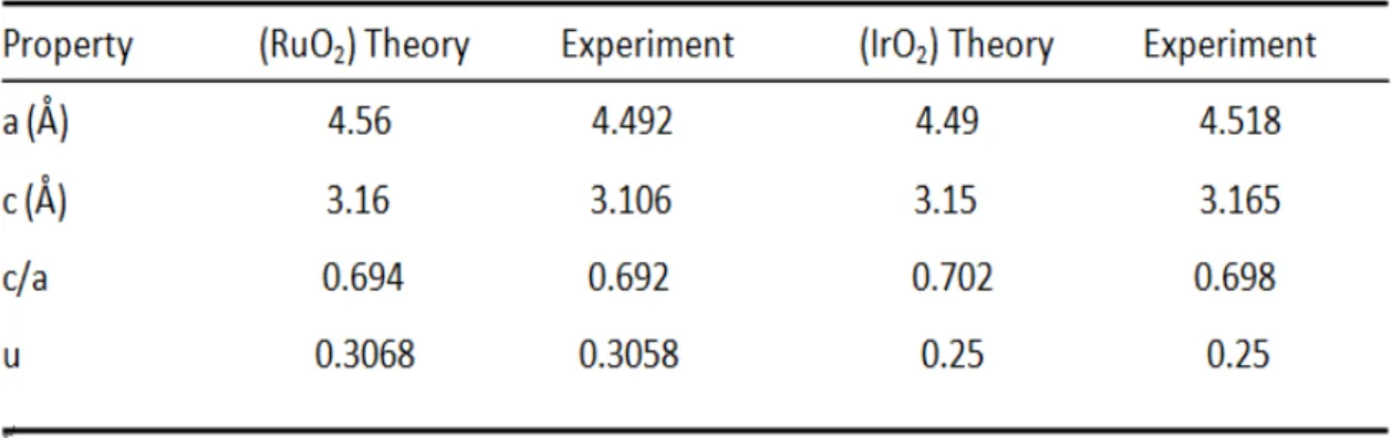
For the RuO2 bulk, the lattice parameters are a=b=4.56 Å, c=3.16 Å in theoretical

calculation which are in good agreement with the experimental values, a=b=4.500±0.005 Å, c=3.101±0.006 Å. Similarly in the case of the IrO2 bulk material,

the lattice parameters for theoretical value are a=b=4.49 Å, c=3.15 Å which is in good agreement with the experimental values: a=b=4.518 Å, c=3.165 Å. The two Ru and

Ir atoms occupy the sites, (0, 0, 0; , , )1 1 1

2 2 2 , and the four O atoms occupy the sites, 1 1 1

( , , 0; , , ) 2 2 2 u u u u

± + − , where uis an internal parameter and along with a and c/a

describe the oxygen octahedral surrounding each Ru and Ir atom. We summarize the lattice parameters a, c, c/a and for the and

TABLE 1. Comparison of structural parameters for the RuO2 and IrO2 in the rutile

structure obtained from the experimental measurements and the theoretical calculations2_.

Fig. 3.1 The primitive cells for RuO2(upper panel) and IrO2 (lower panel) in the rutile

structures.

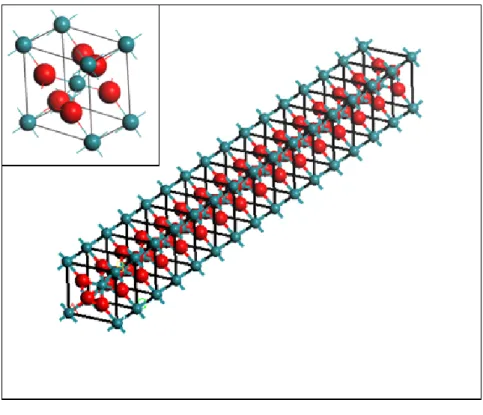
For the bulk the primitive cell is periodic permutation in the x, y and z direction. We then build up the 1x1 and 2x2 nanowires along the (001) direction from the structure of the bulk crystal. It has the same periodicity along the z direction for 1x1 nanowires. The periodic permutation for 1x1 nanowires is one primitive cell and two empty primitive cells along the x and y direction. Thus, the lattice parameters become a=b=13.68 Å, c=3.16 Å for the RuO and a=b=13.47 Å, c=3.15 Å for the 2 IrO2. The

Fig. 3.2 The structure of 1x1 nanowire for RuO2 (upper panel) and IrO2(lower panel).

The picture of the top-left corner is its bulk structure.

The 2x2 nanowires have the same periodicity along the z direction as the bulk crystal. The periodicity of 2x2 nanowires is two repeated primitive cells and two empty primitive cells along the x and y direction. Thus, the lattice parameters become a=b=18.24 Å, c=3.16 Å for the RuO2 and a=b=17.96 Å, c=3.15 Å for the IrO2. We

Fig. 3.3 The structure of 2x2 nanowire for RuO2 (upper panel) and IrO2(lower

panel).

The reason for the repetition of two empty primitive cells in the x and y direction nanowires is to avoid the interactions between wires. It must be greater than 9 Å which is about the size of the two primitive cells.

3-2 VASP Calculation

In the previous section, we have introduced the structures of the RuO2 and 2

IrO . We relax the structures of the RuO₂ and _{IrO by applying the VASP code. 2} VASP is an ab-initio package for performing quantum mechanical molecular dynamics simulations using the pseudopotential or the projector-augmented wave method and a plane wave basis set. The approach implemented in VASP is based on the local density approximation with the free energy variational quantity. Forces can be calculated with VASP and used to relax atoms into their ground state.

VASP have four input files, INCAR, KPOINTS, POSCAR, and POTCAR. The POSCAR file contains the lattice geometry and the atom positions. We apply the software “Material Studio” to construct the positions of atoms in the crystal material and nanowires. The results of the coordinates obtained from the “Material Studio” have entered into the POSCAR file in VASP. The example is shown in Fig.3.4.

Fig. 3.4 The contents of the POSCAR file.

The first line is treated as a comment line. The data from the third to fifth lines are the lattice constants for a, b and c respectively. The data from the eighth to final lines are the positions of atoms in Cartesian coordinates.

The POTCAR file contains the pseudopotential for each atomic species used in the calculations. The file is large, so we only show the partial contents of the POTCAR file.

Fig. 3.5 The partial contents of POTCAR file for local-density approximation.

The KPOINTS file contains the coordinates and weights of the k-point mesh. We choose the default settings to generate k-point, and we only need to specify the subdivisions in the first Brillouin zone in each direction. The content of the KPOINTS file is shown in Fig.3.6.

Fig. 3.6 The contents of the KPOINTS file.

The first line is treated as a comment line. In the second line, the number 0 is specified to generate the k-point automatically. The third line starting with “M” selects the Monkhorst-Pack scheme for k-points. The fourth line shows (10 10 10) which means to generate 10x10x10 k-point in the first Brillouin zone.

The INCAR file is the most important input file in VASP. It contains a lot of useful parameters. We only show in Fig.3.7 the parameters other than the default values in the INCAR file.

Fig. 3.7 The contents of the INCAR file.

On the first line it contains the job title which can be arbitrarily named. When we run a new job, ISTART must be set to 0. One can set the “PREC=High or Accurate” to increase the precision in the calculations at cost of more computer time. ISMEAR in the INCAR file determines how the partial occupancies fnk are set for each wave function.

We choose the ISMEAR equal to 1 according to the recommendation by the VASP manual, which recommends that the metals use ISMEAR=1 in the relaxation processes. The conductivities of RuO2 and IrO2 are close to the properties of metal. The tag

NSW defines the number of ionic steps. We do not display other parameters which are set to the default values.

With the four input files in VASP, the jobs can be submitted to PC Clusters for calculations. The output files are shown in Fig.3.8.

Fig. 3.8 All output files of the VASP.

To calculate the force constants we need to move the positions of atoms, which are stored in the file CONTCAR containing the information of atom positions after relaxation. The OUTCAR file contains other useful information such as forces, potentials, free energy, etc.

phonon dispersion relation of the crystal. The program “PHON” is able to calculate the phonon dispersion relations incorporated with any other program which is capable of calculating the force matrices of the system.

The program “PHON” has three input files, INPHON, FORCES and POSCAR. The POSCAR file of the program “PHON” needs the relaxed atom positions which are given by the CONTCAR file, one of the output files in the VASP program.

The INPHON file is the central input file of “PHON”. The parameters in the INPHON file are shown in Fig.3.9.

Fig. 3.9 The contents of the INPHON file.

Most of the parameters are set to the default values. It should pay attention to the LSUPER tag which must be set to LSUPER=.T. in the INPHON file. In the trial run of “PHON” program, we only need two files POSCAR and INPHON where the tag LSUPER is set to “True”. The trial run will generate the DISP file, where the displacement vectors of the atoms are given. These displacement vectors tell us how to move the positions of atoms and are applied to calculate the force matrices by using the VASP

program. The example of the DISP file is shown in Fig.3.10.

Fig. 3.10 The contents of the DISP file.

The first line contains the information of how the atoms must be displaced. The 1 and 3 in the first column represent the first atom and the third atom, respectively. The three numerals in the second to fourth columns represent the relative displacement vectors of atoms. When we have these data, we reconstruct the POSCAR in the VASP program using the relaxed coordinates of atoms from the CONTCAR file in the VASP program and displacement vectors in the DISP file from the PHON program. We fix the atoms positions after moving the atoms and run the VASP program again to obtain the force matrices.

The FORCES file contains the displacements and the force information of each atom. We obtain the force matrices after the system relaxed by VASP. The example is shown in Fig. 3.11.

Fig. 3.11 The contents of the FORCES file.

The number of the first line is specified the number of displacements. The second line contains the information of how the atoms must be displaced. The data from the third to eighth line are the forces on all the atoms in the supercell. According to the information of the DISP file, there are four force matrices in the FORCES file.

Before we run the PHON, the tag LSUPER in the INPHON file must be set “F”. With the three input files, the jobs can be submitted to PC Clusters for calculations. The results are shown in Fig. 3.12.

Fig. 3.12 Phonon dispersion relation for the RuO2(upper panel) and IrO2(lower

optical branches. There are twelve acoustic branches and sixty optical branches in the 2x2 nanowires. The value of sound velocity plays an important part in our study. The sound velocity is obtained from the phonon dispersion relation. The group velocity of the phonon is defined as g

d V

dk

ω

= , so we are able to calculate the sound velocity from the phonon dispersion relation of the the acoustic phonon. These quantities will be used late to calculate the resistivity of the bulk materials and nanowires.

3-4 Matthiessen’s rule

Theoretically, the resistivity is defined as

2 4 , p π ρ τ = Ω (3.1) where 1

τ is the electron scatter rate and Ωp is the plasma frequency. The plasma

frequency tensor can be calculated from knowledge of the electronic structure and is given by 2 2 8 2 , nk p nk nk nk f e V π _υ ε ∂ − Ω = ∂

∑

where V is the volume, the group velocity of phonon is 1 nk nk k ε υ = ∂ ∂  and fnk is the

particle distribution function. The scattering rate for electron transport resulting from electron-phonon scattering is given by

2 2 0 / 2 4 ( )[ ] , sinh( / 2 ) B B B k T d k T F k T ω ω π α ω τ ω ω ∞ =

∫

where ω is the phonon frequency and 2

( ) F

α ω is the spectral function.

Typically, the scattering rate for many metals follows a Bloch-Gruneisen type behavior. For acoustic mode phonons, 2

( ) F

α ω will be replaced with its Debye approximation： 2 4 ( ) 2 ( ) ( ), BG BG D D F ω α ω λ θ ω ω ω = − (3.4)

where θ is the Heaviside step function, ωD is the Debye frequency and λ is the BG

transport electron-phonon coupling constant in the Bloch-Gruneisen model26. One can plug Eq. (3.4) into Eq.(3.3) and obtain the scattering rate

2 2 0 2 4 0 ₂ 5 4 0 ₂ / 2 8 ( ) ( )[ ] sinh( / 2 ) 8 ( ) [ ] 4 sinh ( ) 2 8 ( ) , 4 sinh ( ) 2 D D B B BG D BG D B T B BG D T B BG D k T d k T k T dx T x k T x x x T x k T dx x ω ω ω π λ θ ω ω τ ω ω ω π λ π λ ∞ Θ Θ = − = Θ = Θ

∫

∫

∫

Here, Θ is the Debye temperature corresponding to the maximum phonon D

energy in the Debye approximation. Substituting Eq.(3.5) and Eq.(3.2) into Eq.(3.1), the resistivity can be written as

2 5 4 2 ₀ 2 32 ( ) ( ) . 4 sinh ( ) 2 D T BG B BG p D T x T k T dx x π ρ = λ Θ Ω Θ

∫

If the temperature is smaller than Debye temperature, the result of the integral equation approaches to a constant, and thus the resistivity in the Bloch-Gruneisen model is proportional to 5

T . The above equation is applied to calculate the resistivity of the RuO2 and IrO2nanowires.

An additional contribution due to the coupling between electrons and optical mode phonons can be considered as well. The electron-phonon contribution can be obtained by substituting 2

( )

EF

α ω in the Einstein approximation.

2 1

( ) ( ).

2

EF E E E

Substituting Eq.(3.7) into Eq.(3.3) , the equation is shown as 2 0 2 2 / 2 2 ( )[ ] sinh( / 2 ) / 2 2 [ ] sinh( / 2 ) / 2 2 [ ] , sinh( / 2 ) E B B E E E B E B B E E B E B E E k T k T d k T k T k T k T T k T T ω ω π λ ω δ ω ω τ ω ω ω π λ ω π λ ∞ = − = Θ = Θ

∫

From Eq.(3.8) and Eq.(3.2) the resistivity is given by

2 2 / 2 8 ( ) [ ] . sinh( / 2 ) E E B E p E T T k T T π ρ = λ Θ Ω Θ  (3.9)

The optical mode coupling term is treated using Einstein approximation with a single phonon frequency corresponding to the energy kBΘ . E

Besides the electron-phonon scattering, there is another term to influence the resistivity which is electron-electron scattering. The resistivity depends on 2

T and can be written as 2 ( ) . ee T A Tee ρ = (3.10)

According to the Matthiessen’s rule these three contributions [Eq.(3.6), Eq.(3.9), Eq.(3.10)] are additive and independent of each other. The total resistivity ( )ρ T is the sum of the residual resistivity ρ , Eq.(3.6), Eq.(3.9) and Eq.(3.10), it can be 0

expressed as follow.

0

( )T _BG( )T _E( )T _ee( ).T

ρ =ρ +ρ +ρ +ρ (3.11)

At low temperature, the resistivity is dominated by impurities, vacancies, and various other defects. For low defect concentrations, these contributions are frequently assumed to be independent of the temperature; the T=0 limit being defined as the residual resistivity ρ . The resistivity due to the electron-electron scattering 0

parameter Aee is only of the order of

5 2

10 (− µΩ ⋅cm K/ ).

3-5 Results and Discussion

3-5-1 Debye temperature calculation

The Debye temperature is defined as

1 2 3 6 ( ) , D B N k V υ π Θ =  (3.12)

where υ is the velocity of sound, N is the number of primitive cells in the sample and V is the volume of the sample. From the phonon dispersion relation together with the parameters known from the structures of nanowires, we can calculate the sound velocity υ and the Debye temperature from our theoretical calculations.

The temperature dependence of the resistivity at T < Θ is determined by the D

electron-phonon contribution only. When the ratio of D

T Θ

is large, the resistivity is proportional to 5

T . Oppositely, the ratio of D

T Θ

is small, the resistivity gives a T dependence. Our research is focus on the resistivity varies as 5

T in Bloch- Gruneisen equation. Thus, the low temperature system is mainly investigated for us. The results are shown in Fig.3.13 and we can see that the Debye temperature increases as the sizes of the system increase.

Fig. 3.13 The dependence of the Debye temperature in RuO2 (upper panel) and IrO2

3-5-2 Bloch-Gruneisen Model calculation

We investigate the resistivity of the nanowires due to the electron-phonon scattering. It gives a 5

T dependence at low temperature. The results of the resistivity versus the temperature in RuO2 and IrO2 are shown in Fig.3.14.

Fig. 3.14 The resistivity of RuO2 (upper panel) and IrO2 (lower panel) nanowires

due to the interactions between electrons and the acoustic phonons.

From the frequency dispersions, we observe that the velocity of phonon in the 1x1 nanowire is the slowest. The sound velocities increase as the diameters of the wires increase. From the approximately expression k

m

ω= for a harmonic oscillator from the Hooke’s law, we realize that the sound velocity decreases as the force constants decrease. We conjecture that the nanowires with smaller diameters have smaller binding force and smaller sound velocity, and thus are less stable.

At low temperatures, we observe that the resistivity increases as the temperature rises. The lattice vibrations are more violent as the temperatures rise, which generate more phonons. Consequently, the probability of electron-phonon collision increases and it causes the conductivity to decrease. The resistivity varies with 5

T according to the Bloch-Gruneisen equation. At a given temperature, the resistivity decreases as the diameter of the nanowire. The decrease of the sound velocity is due to the decrease of the effective strength of the force which binds the nanowire.

Chapter4 Conclusion

We have investigated the Debye temperature and the conductivity for RuO2

and IrO2 nanowires due to the electron-phonon interactions described by the

Bloch-Gruneisen theorem.

Firstly, we employ the projected augmented wave method as implemented in Vienna Ab initio Simulation Package (VASP) to investigate systems of RuO2 and

2

IrO bulk crystal using density-functional theory calculations with exchange correlation energy in the local density approximation. All atoms are relaxed until the forces are smaller than 0.001 eV/Å. The optimized the RuO bulk crystal has lattice 2

parameters: a=b=4.56 Å, c=3.16 Å, which are in good agreement with the experimental values, a=b=4.500±0.005Å, c=3.101±0.006 Å. In the same way we relax the geometry for the IrO bulk crystal, and obtain the lattice parameters: a=b=4.49 Å, c=3.15 Å, 2

which are also in good agreement with the experimental values.

Secondly, we build up the super cell structures of nanowires along (001) direction based on the geometry of the relaxed bulk systems as the initial input. We have built up two different diameters of RuO2 and IrO2 nanowires: (1) one unit cell (1×1) and

(2) four unit cells (2×2) in the directions parallel to the direction of charge current. Nanowires are infinite along the (001) direction and are also separated by a vacuum region in the x and y directions. We also relax the geometry of nanowires following the same method using VASP as described in the above, where have used (1×1×10) k-point Monkhorst-Pack meshes in our calculations.

The VASP is applied to calculate the force matrix and the PHON is applied to calculate the phonon dispersion relations of the bulk and nanowires. For the IrO2

system, the Fermi energies of the bulk crystal, 1x1 wire, and 2x2 wire are 6.19 eV, 5.84 eV, and 3.39 eV, respectively. Since the diameters of the nanowires (4.49 Å for bulk crystal and 13.47 Å and 17.96 Å for 1x1 and 2x2 wires, respectively) are comparable with the Fermi wave lengths, the systems may display strong quantum mechanical effects. We observe that the sound velocities and the Debye temperatures are strongly suppressed when the decreasing diameters of the nanowires are comparable to the Fermi wave lengths.

Using the phonon dispersion obtained from the PHON and VASP, we calculate the conductivities of nanowires due to the interactions between electrons and the vibrations of lattice. The resistivity varies as 5

T at low temperatures according to the Bloch-Gruneisen equation. At a given temperature, we observe that the conductivity due to electron-phonon interactions decreases as the diameters of nanowires