Price and Volatility Spillovers between Stock Prices and Exchange Rates: Empirical Evidence from the G-7 Countries

Price and Volatility Spillovers between Stock Prices and Exchange

Rates: Empirical Evidence from the G-7 Countries

Sheng-Yung Yang*

Department of Finance, National Chung Hsing University, Taiwan

Shuh-Chyi Doong

Department of Finance, National Chung Hsing University, Taiwan

Abstract

This paper explores the nature of the mean and volatility transmission mechanism between stock and foreign exchange markets for the G-7 countries. Empirical evidence supports the asymmetric volatility spillover effect and shows that movements of stock prices will affect future exchange rate movements, but changes in exchange rates have less direct impact on future changes of stock prices. The implication is particularly important to international portfolio managers when devising hedging and diversification strategies for their portfolios.

Key words: exchange rate; stock price; bivariate EGARCH model; asymmetric volatility

spillover

JEL classification: C22; F31; G12

1. Introduction

The rapid expansion in international trade since the 1970s, and the adoption of freely floating exchange rate regimes by many industrialized countries in 1973, heralded a new era of increased exchange rate risk and volatility. Not surprisingly, the economic exposure of firms to exchange rate risks has increased. In the aggregate sense, stock markets should respond to the excess movement and increasing volatility of exchange rates. Exchange rates are also more sensitive to stock market innovations and global portfolio investments because the rapid integration and deregulation of international financial markets since the 1980s has made the capital flows across borders easier and faster than ever before.

Received December 31, 2003, revised September 2, 2004, accepted October 13, 2004.

*_{Correspondence to: Department of Finance, National Chung Hsing University, 250 Kuo Kuang Road,}

Taichung 402, Taiwan. E-mail: shengyang@nchu.edu.tw. Financial support from the National Science Council of Taiwan (NSC-91-2416-H-005-017) is gratefully acknowledged. We are grateful to two anonymous referees and the managing editor of the journal for valuable comments and suggestions that helped us significantly improve the paper.

In recent finance literature, the dynamic relationship between stock prices and exchange rates has drawn much attention from financial economists and practitioners since both variables play crucial roles in portfolio decisions and economic development. Theoretical links between stock prices and exchange rates have taken two forms. First, the “flow-oriented” models of exchange rates (e.g., Dornbusch and Fischer, 1980) focus on the current account or the trade balance. These models posit that changes in exchange rates affect international competitiveness and trade balances, thereby influencing real income and output. Stock prices, generally interpreted as the present values of future cash flows of firms, react to exchange rate changes and form the link among future income, interest rate innovations, and current investment and consumption decisions. Innovations in the stock market, on the other hand, affect aggregate demand through wealth and liquidity effects, thereby influencing money demand and exchange rates (Gavin, 1989).

The second approach involves the “stock-oriented” models of exchange rates (e.g., Branson, 1983; Frankel, 1983). These models view exchange rates as equating the supply and demand for assets such as stocks and bonds. This approach gives the capital account an important role in determining exchange rate dynamics. Since the values of financial assets are determined by the present values of their future cash flows, expectations of relative currency values play a considerable role in their price movements, especially for internationally held financial assets. Therefore, stock price innovations may affect, or be affected by, exchange rate dynamics.

Early empirical studies have focused on the contemporaneous relation between stock returns and exchange rates. Aggarwal (1981) finds that US stock prices and the trade-weighted dollar are positively correlated. In contrast, Soenen and Hennigar (1988) document a strong negative correlation between US stock indexes and a fifteen currency-weighted value of the dollar. Ma and Kao (1990) provide some insights into probable reasons for these different correlations. They include six industrial economies to investigate the impact of changes in currency values on stock prices. Their results suggest that for an export-dominant economy, currency appreciation has a negative effect on the stock market, while currency appreciation boosts the stock market for an import-dominant economy.

More recently, studies have focused on the interactions or the directions of causality between exchange rates and stock prices for major industrial economies. Bahmani-Oskooee and Sohrabian (1992) show that there is bidirectional causality between stock prices measured by the S&P 500 index and effective exchange rates of the dollar. Ajayi and Mougoué (1996) find significant short-run and long-run feedback relations between the two variables for eight industrial economies. Specifically, their results show that an increase in stock prices has a negative short-run and a positive long-run effect on domestic currency value while currency depreciation has negative short- and long-run effects on the stock market. Ajayi et al. (1998) provide evidence to indicate unidirectional causality from the stock to the currency markets for advanced economies and no consistent causal relations in emerging markets. Chiang et al. (2000) show that stock returns and currency values

are positively related for nine Asian markets. Nieh and Lee (2001) find significant short-run dynamics and no long-run relationship between stock prices and exchange rates for the G-7 countries. To date, however, empirical investigations are at best scant and inconclusive.

Despite the examination of the linkages and interactions between exchange rates and stock prices, only a limited body of research has attempted to analyze the possibility that the transmission of volatility or a volatility spillover effect can exist between the stock and currency markets. An examination of the volatility spillover process also enhances the understanding of information transmission between stock prices and exchange rates. The recent economic globalization and integration of world financial markets, fueled by the development of information technology, increases the international transmission of returns and volatilities among financial markets. A rich empirical literature exists on the examination of the stochastic behavior of stock prices and exchange rates, primarily employing the autoregressive conditional heteroskedastic (ARCH) methodology of Engle (1982); see Bollerslev et al. (1992) for a detailed summary of the literature. In addition, these and Generalized ARCH (GARCH) models have been used to study volatility spillovers between markets in different countries and between different assets. For example, Hamao et al. (1990) investigate the price and volatility spillovers in three major stock markets (New York, Tokyo, and London). Koutmos and Booth (1995) find asymmetric volatility spillovers across the same stock markets. Chiang and Yang (2003) show that the volatility of stock returns displays not only a clustering phenomenon but also a significant spillover effect between the US and major world stock markets. Laopodis (1998) explores the nature of the volatility transmission mechanism of exchange rates. So (2001) studies the dynamic spillover effect between interest rates and the exchange value of the US dollar.

This paper adopts a bivariate EGARCH framework and investigates the dynamic price and volatility spillovers between stock prices and exchange rates for the G-7 countries. The framework can help not only to understand the short-run movements but also to investigate the volatility transmission mechanism between the two markets. Also, it allows the quantity (size) and the quality (sign) of an innovation to seriously affect the extent of volatility spillovers across markets. We attempt to fill the gap in the literature by investigating how information is transmitted between these two financial variables through short-term price interaction and asymmetric volatility spillovers. Improved knowledge of the price and volatility spillover effect between the stock and currency markets, and consequently the degree of their integration, will expand the information set available to international portfolio managers, multinational corporations, and policymakers for decision-making.

The rest of the paper is organized as follows. Section 2 discusses the data sources and the methodological design of the study, and Section 3 analyzes the empirical findings. Section 4 summarizes the study and concludes with some general remarks.

2. Data and Methodology 2.1 Data

The data set consists of weekly (Friday) closing exchange rates and stock market indices for the G-7 countries. The stock indices for the G-7 countries are Toronto 300 Composite, Paris CAC 40, Frankfurt DAX, Milan Stock Index, Nikkei 225, FT-100, and S&P 500 from Datastream International. The exchange rate series are from the WEFA groups and are stated in US dollars per local currency (note that the trade-weighted value index of the US dollar is constructed to proxy for exchange value of the dollar). The sample period runs from 01/05/1979 to 01/01/1999, yielding 1045 observations. The rationale for the starting date is that it coincides with the beginning of EMS operations, while the end point is dictated by the availability of data. Also, it is noted that the European Monetary Union (EMU) was created with the launching of the euro on January 1999. Using weekly data in this study is justified since data of high frequency (e.g., daily or intraday) contains too much noise, while too wide a time grid (e.g., monthly or quarterly) does not capture the information content of changes in stock prices and exchange rates. Therefore, the sample period enables us to explore the short-term dynamic relationships between stock prices and exchange rates at the time of floating exchange rate regimes and the era of increasing integration of financial markets.

Rates of change of the data series are calculated as ) ln( 100 , , 1 ,t= × it it− i P P R , (1)

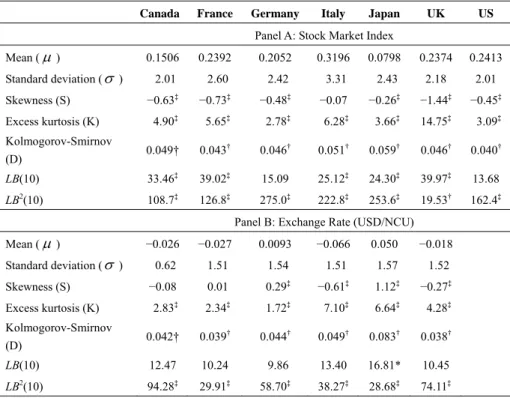
where Pi,t is the price level of market i (i = 1 for the stock market and i = 2 for the foreign exchange market) at time t. Table 1 reports summary statistics. The sample means for all markets are not statistically different from zero. The measures for skewness and excess kurtosis show that most return series are negatively skewed and highly leptokurtic with respect to the normal distribution. The Kolmogorov-Smirnov statistics reject normality for each of the series at the 5 percent level of significance. The Ljung-Box statistics for up to 10 lags, calculated for both the return and squared return series, indicate the presence of significant linear and non-linear dependencies. Linear dependencies may be due to some forms of market inefficiency or market structure, and non-linear dependencies may be due to autoregressive conditional heteroskedasticity.

2.2 Methodology

To model the short-run dynamic relationships between stock prices and exchange rates, we use the following Vector Autoregressive (VAR) model:

∑ +∑ + + = = − − = − − 2 1 2 1 , 2 , 2 , 1 , 1 , 0 , , j ijt jt j ijt jt it i t i R R R β β β ε for i, j = 1, 2. ₍₂₎

In the above model, β , i,0 βij,t−1, and βij,t−2 are parameters to be estimated and εi,t is the residual. By construction, news in market i becomes part of the information set in market j so it can be exploited by the stock and foreign exchange markets. Accordingly, coefficients β for i ≠ j, if statistically significant, reflect the extent ij of price (mean) spillovers across markets; i.e., the price informational efficiency.

Table 1. Descriptive Statistics of Weekly Changes in Stock Market Index and Exchange Rate Canada France Germany Italy Japan UK US

Panel A: Stock Market Index

Mean (µ) 0.1506 0.2392 0.2052 0.3196 0.0798 0.2374 0.2413 Standard deviation (σ ) 2.01 2.60 2.42 3.31 2.43 2.18 2.01 Skewness (S) −0.63‡ _−0.73‡ _−0.48‡ _{−0.07 −0.26}‡ _−1.44‡ _−0.45‡ Excess kurtosis (K) 4.90‡ _5.65‡ _2.78‡ _6.28‡ _3.66‡ _14.75‡ _3.09‡ Kolmogorov-Smirnov (D) 0.049† 0.043 † _0.046† _0.051† _0.059† _0.046† _0.040† LB(10) 33.46‡ _39.02‡ _{15.09 25.12}‡ _24.30‡ _39.97‡ _13.68 LB2_{(10) 108.7}‡ _126.8‡ _275.0‡ _222.8‡ _253.6‡ _19.53† _162.4‡

Panel B: Exchange Rate (USD/NCU)

Mean (µ) −0.026 −0.027 0.0093 −0.066 0.050 −0.018 Standard deviation (σ ) 0.62 1.51 1.54 1.51 1.57 1.52 Skewness (S) −0.08 0.01 0.29‡ _−0.61‡ _1.12‡ _−0.27‡ Excess kurtosis (K) 2.83‡ _2.34‡ _1.72‡ _7.10‡ _6.64‡ _4.28‡ Kolmogorov-Smirnov (D) 0.042† 0.039 † _0.044† _0.049† _0.083† _0.038† LB(10) 12.47 10.24 9.86 13.40 16.81* 10.45 LB2_{(10) 94.28}‡ _29.91‡ _58.70‡ _38.27‡ _28.68‡ _74.11‡

Note: *, †_{, and} ‡ _{denote significance at the 10%, 5%, and 1% level, respectively. All changes (returns) are} expressed in percentages. The test statistics for skewness and excess kurtosis are the conventional t- statistics. LB(10) and LB2_{(10) are the Ljung-Box statistics for returns and squared returns, respectively,}

with both distributed chi-square with 10 degrees of freedom. The normal density is assumed for the Kolmogorov-Smirnov statistics.

The optimal lag length for a VAR model is usually based on some information criteria and/or residual tests. After considering the parsimony principle and the residuals’ white-noise property, a two-period lag or VAR(2) model is selected.

As explained above (see Table 1), since the returns of the two markets exhibit very strong ARCH effects, we model the conditional variances of and volatility spillovers between the two markets through a multivariate version of Nelson’s (1991) Exponential GARCH (EGARCH) model. Competing models which also capture the asymmetric effect include GJR-GARCH and Quadratic GARCH models. However, a significant body of evidence, summarized by Hamilton (1994, p. 672), supports the use of the EGARCH model. One nice feature of the EGARCH model is the log form

of conditional variance, thereby guaranteeing that the variance is positive. Other multivariate GARCH models such as the GJR model need to have parameter restrictions to ensure the non-negativity of conditional variances. Following Koutmos and Booth (1995), we model the conditional variances between stock prices and exchange rates according to the following bivariate EGARCH model:

( )

( )

( )

(

)

The persistence of volatility implied by equation (3) is measured by γ . The i unconditional variance is finite if γ < 1. The conditional variance process given by i equation (3) allows its own lagged and cross-market standardized innovations to exert an asymmetric impact on the volatility of market i. The coefficient α (for i ≠ ij j) captures the volatility spillover effect. For example, if α is significantly 12

different from zero, then volatility of exchange rates will spillover to that of stock prices. Asymmetry is modeled by equation (4) where zj,t−1 is the standardized

residual at time t−1, which is defined as εj,t−1 σj,t−1, and E(zj,t−1) is the expected

absolute value of zj,t−1. The parameter δ in equation (4) measures the asymmetric j impact on the volatility of market i with the following partial derivatives:

( )

( )

Intuitively, asymmetry exists if δ is negative and statistically significant. j The term |z_{j t, 1−} |−E z(| _{j t, 1−} |) measures the size effect of an innovation whereas

1 ,t−

j jz

δ measures the corresponding sign effect. A negative δ with positive and j significant α implies that a negative shock in market i increases volatility in ij market j more than a positive shock of an equal magnitude. The reverse holds true for positive values of δ . Such a result would reveal the asymmetric nature of the j spillover mechanism. Further, a negative (positive) zj,t coupled with a negative

j

δ enhances (reduces) the size effect. The relative importance of asymmetry or a leverage effect can be measured by the ratio |−1+δj| (1+δj). This ratio also considers the differing impact of a market’s own innovation on the current conditional variance. Thus, a negative value of δ magnifies the ratio. This j indicates that negative innovations will have greater impacts on conditional volatility than positive innovations. Economically, this means that unexpected “bad” news (negative innovations) will have greater impacts on current conditional

volatility than “good” news (positive innovations).

Finally, the residuals of equation (2) are assumed to be normal and the conditional covariance specification is presupposed to be constant correlation coefficients (Bollerslev, 1990). The interpretation should be based on the fact that they measure contemporaneous relationships. This is equivalent to saying that the covariance is commensurate to the product of the standard deviations as described by the following equations:

(

)

where It−1 is the information set at time period t−1 and Ht is the conditional variance-covariance matrix at time t. The specification reduces the number of parameters to be estimated and makes the estimation more tractable. And, with the assumption of normality, the log-likelihood function of the multivariate EGARCH model is expressed as:

(

)

where N is the number of equations (two here), T is the number of observations, and θ is the 1×21 vector of parameters to be estimated. The log likelihood function is estimated using the Berndt et al. (1974) algorithm via Quasi-Maximum Likelihood Estimation (QMLE). As shown by Bollerslev and Woolridge (1992), QMLE is consistent with a limiting normal distribution if the conditional mean and variances are appropriately specified, though asset returns are not normally distributed. Following Bollerslev and Woolridge, robust standard errors are calculated to take into consideration non-normality of the residuals.

3. Empirical Findings

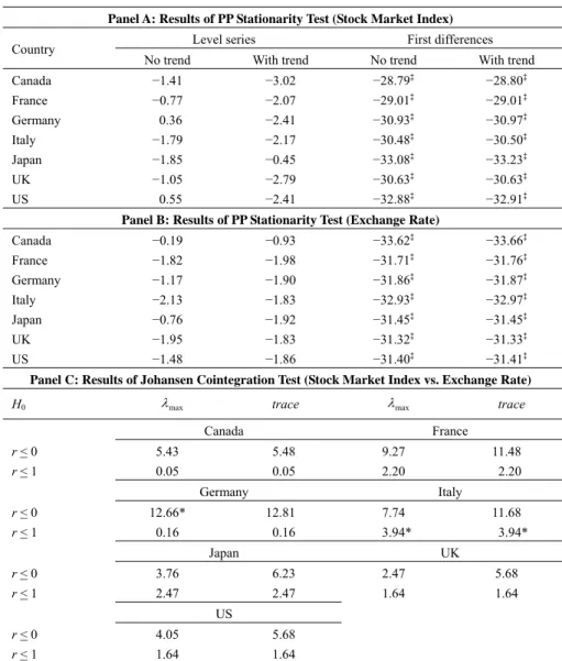
Before the above VAR model is estimated, it is necessary to check stationarity of the variables and a possible cointegration relation between them. This step is essential since error correction terms should be incorporated in the above VAR model if the series are cointegrated (Engle and Granger, 1987). To test for stationarity of the series, we use the Phillips-Perron (PP) test since there are autocorrelation and ARCH effects in the series, and the PP test is robust to strong autocorrelation and heteroskedasticity. We use the Johansen test to examine if the two variables are cointegrated. The Johansen test is used here as it is also shown to be robust in the presence of heteroskedasticity (Lee and Tse, 1996). From the results in Panels A and B of Table 2, the level series of data are not stationary, whether or not a time trend is included in the calculation of the test statistics. When the first

differences of the series are taken, the PP test statistics become significant. Therefore, the series are I(1) processes and they are integrated of the same order.

Table 2. Results of PP Stationarity Test and Johansen Cointegration Test Panel A: Results of PP Stationarity Test (Stock Market Index)

Level series First differences

Country

No trend With trend No trend With trend

Canada −1.41 −3.02 −28.79‡ _−28.80‡ France −0.77 −2.07 −29.01‡ _−29.01‡ Germany 0.36 −2.41 −30.93‡ _−30.97‡ Italy −1.79 −2.17 −30.48‡ _−30.50‡ Japan −1.85 −0.45 −33.08‡ _−33.23‡ UK −1.05 −2.79 −30.63‡ _−30.63‡ US 0.55 −2.41 −32.88‡ _−32.91‡

Panel B: Results of PP Stationarity Test (Exchange Rate)

Canada −0.19 −0.93 −33.62‡ _−33.66‡ France −1.82 −1.98 −31.71‡ _−31.76‡ Germany −1.17 −1.90 −31.86‡ _−31.87‡ Italy −2.13 −1.83 −32.93‡ _−32.97‡ Japan −0.76 −1.92 −31.45‡ _−31.45‡ UK −1.95 −1.83 −31.32‡ _−31.33‡ US −1.48 −1.86 −31.40‡ _−31.41‡

Panel C: Results of Johansen Cointegration Test (Stock Market Index vs. Exchange Rate)

H0 λmax trace λmax trace

Canada France r < 0 5.43 5.48 9.27 11.48 r < 1 0.05 0.05 2.20 2.20 Germany Italy r < 0 12.66* 12.81 7.74 11.68 r < 1 0.16 0.16 3.94* 3.94* Japan UK r < 0 3.76 6.23 2.47 5.68 r < 1 2.47 2.47 1.64 1.64 US r < 0 4.05 5.68 r < 1 1.64 1.64

Note: *, †_{, and} ‡ _{denote significance at the 10%, 5%, and 1% level, respectively,}

0

H is the null

hypothesis that the number of cointegrating vectors is less than or equal to numbers specified, and λmax

and trace are Johansen test statistics for testing cointegration.

Since they are integrated of the same order, the Johansen test is used to examine if the two variables are cointegrated. Panel C of Table 2 contains the test results. The test results here show that stock market indices and exchange rates are not cointegrated; hence, the VAR model in equation (2) is well specified with no

need to include error correction terms. In contrast with Bahmani-Oskooee and Sohrabian (1992) and Ajayi and Mougoué (1996), our result is consistent with Granger et al. (2000) and Nieh and Lee (2001) that there is no lung-run significant relationship between stock prices and exchange rates.

3.1 Results from the Multivariate EGARCH Model

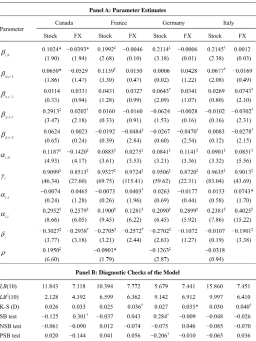
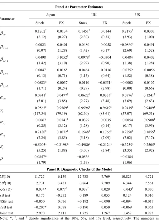
The maximum likelihood estimates of the multivariate model are reported in Table 3. The model considers both price and asymmetric volatility spillovers between the stock and foreign exchange markets. For the first moment interdependencies, there are significant price spillovers from foreign exchange to the stock market for Canada and Japan. Currency depreciation (appreciation) often drags down (up) stock prices for Canada and Japan. In the long run for an economy with a significant import (export) sector, the unfavorable effects of currency depreciation (appreciation) on imports (exports) may induce a bearish stock market. However, in the short run, currency depreciation may have a negative effect on the stock market because the domestic counterpart of currency depreciation is inflation, which may exert a dampening effect on the stock market. In addition, the inflationary effects of a declining domestic currency may encourage international investors to decrease their portfolio of domestic assets, thereby depressing the stock market in the long run. There are also significant price spillovers from the stock market to the exchange market for Canada, France, Germany, Italy, and the UK. An increase (decrease) in stock price often causes currency depreciation (appreciation) for the next week or two for France, Germany, Italy, and the UK. The short-run effect of increases in stock prices on domestic currency value can be explained by the stock market’s providing a barometer for the health of an economy (Solnik, 1987). A bullish market reflects economic expansion, and this tends to fuel inflation expectations. An increase in inflation expectation exerts downward pressure on the value of the domestic currency in the short run. In the long run, however, the positive effect of an increase in stock prices on exchange rates is consistent with the asset view of exchange rates. Our focus is on the short-term dynamic between the variables, and the findings are similar to those of Ajayi and Mougoué (1996) and Nieh and Lee (2001). In general, for the G-7 countries, the results imply that changes in stock prices signal important information about the economic fundamentals to the foreign exchange market, but exchange rate movements do not convey much information about future stock price movements.

Turning to the second moment interdependencies, it can be seen that there exists volatility spillover from the stock to foreign exchange markets for France, Italy, Japan, and the US. And we find no volatility spillover from the foreign exchange to the stock markets at all. In terms of asymmetric spillover effects, negative innovations in the stock market have greater impacts on the conditional volatility of exchange rates than positive innovations for France, Italy, Japan, and the US. However, the effects do not apply to innovations in exchange rates on the stock markets. In the literature, the interactions of stock price and exchange rate changes have been well documented. However, the interactions of volatility on price

movements are often ignored. Empirical evidence in this study demonstrates that volatility of stock prices have (asymmetric) impacts on price movements of foreign exchange rates. Both price and volatility information from the stock market has pricing impacts on the behavior of exchange rates.

Table 3. Results of the Multivariate EGARCH Model Panel A: Parameter Estimates

Canada France Germany Italy Parameter

Stock FX Stock FX Stock FX Stock FX

0 , i β 0.1024* (1.90) −0.0393* (1.94) 0.1992‡ (2.68) −0.0046 (0.10) 0.2114‡ (3.18) −0.0006 (0.01) 0.2145† (2.38) 0.0012 (0.03) 1 ,t− ii β 0.0650* (1.86) −0.0529 (1.47) 0.1139‡ (3.30) 0.0150 (0.47) 0.0006 (0.02) 0.0428 (1.22) 0.0677† (2.08) −0.0169 (0.49) 2 ,t− ii β 0.0114 (0.33) 0.0331 (0.94) 0.0431 (1.28) 0.0327 (0.99) 0.0643† (2.09) 0.0341 (1.07) 0.0269 (0.80) 0.0743† (2.10) 1 ,t− ij β 0.2913‡ (3.47) 0.0202† (2.18) 0.0160 (0.33) −0.0160 (0.91) −0.0624 (1.53) −0.0028 (0.16) −0.0102 (0.16) −0.0302† (2.31) 2 ,t− ij β 0.0624 (0.65) 0.0023 (0.24) −0.0192 (0.39) −0.0484‡ (2.84) −0.0267 (0.60) −0.0470† (2.54) 0.0083 (0.12) −0.0278† (2.15) 0 , i α 0.1187‡ (4.93) −0.1420‡ (4.17) 0.0883‡ (3.61) 0.0275‡ (3.53) 0.0841‡ (3.21) 0.1141‡ (3.36) 0.0901‡ (3.32) 0.0851‡ (5.56) i γ 0.9099‡ (46.34) 0.8513‡ (27.60) 0.9527‡ (69.75) 0.9724‡ (115.41) 0.9506‡ (59.62) 0.8720‡ (22.31) 0.9635‡ (83.04) 0.9013‡ (43.69) j i, α −0.0074 (0.24) 0.0465 (1.28) −0.0073 (0.26) 0.0403† (1.96) 0.0263 (0.69) −0.0177 (0.44) 0.0153 (0.58) 0.0743* (1.70) i i, α 0.2952‡ (8.66) 0.2579‡ (6.05) 0.1900‡ (9.45) 0.1281‡ (6.22) 0.2090‡ (6.45) 0.2899‡ (5.92) 0.2381‡ (7.86) 0.4025‡ (15.22) i δ −0.3027‡ (3.77) −0.2938† (3.18) −0.2705‡ (3.21) −0.2572† (2.44) −0.2702‡ (2.63) −0.1072 (1.27) −0.0107 (0.19) −0.1901‡ (3.38) ρ 0.1950‡ (6.60) −0.0901* (1.79) −0.1263‡ (2.87) −0.0318 (0.94)

Panel B: Diagnostic Checks of the Model

LB(10) 11.843 7.118 10.394 7.772 5.679 7.441 15.860 7.451 LB2_{(10) 2.128 4.392 6.599 6.362 9.142 6.912 9.997 6.410} K-S (D) 0.026 0.033 0.025 0.036† _{0.027 0.035* 0.030 0.040}† SB test −0.125 0.301† _{−0.037 0.043 0.284}† _{−0.009 −0.048 −0.026} NSB test −0.061 −0.090 0.012 −0.074 −0.075 0.046 −0.085 −0.070 PSB test 0.020 −0.144 0.041 0.056 −0.206† _{−0.010 −0.065 0.036} Joint test 4.642 6.994* 0.162 1.623 9.147† _{0.381 4.094 0.937}

Table 3. Results of the Multivariate EGARCH Model (continued) Panel A: Parameter Estimates

Japan UK US Parameter

Stock FX Stock FX Stock FX

0 , i β 0.1202† (2.12) 0.0134 (0.27) 0.1451† (2.30) 0.0144 (0.33) 0.2175‡ (3.93) 0.0303 (1.00) 1 ,t− ii β 0.0023 (0.07) 0.0401 (1.28) 0.0480 (1.42) 0.0058 (0.17) −0.0860‡ (2.60) 0.0491 (1.52) 2 ,t− ii β 0.0498 (1.42) 0.1052‡ (3.10) 0.0978‡ (2.99) −0.0304 (0.90) 0.0484 (1.38) 0.0402 (1.28) 1 ,t− ij β 0.0047 (0.13) 0.0165 (0.71) −0.0464 (1.15) −0.0116 (0.64) −0.0752 (1.52) −0.0056 (0.38) 2 ,t− ij β 0.0683* (1.71) 0.0057 (0.24) 0.0110 (0.27) −0.0551‡ (2.98) −0.0002 (0.00) 0.0102 (0.66) 0 , i α 0.0741‡ (5.01) 0.0477‡ (3.85) 0.0622‡ (2.77) 0.0333‡ (3.48) 0.0776‡ (3.69) 0.1241‡ (2.63) i γ 0.9563‡ (117.54) 0.9569‡ (79.19) 0.9596‡ (62.60) 0.9619‡ (83.61) 0.9419‡ (57.07) 0.9489‡ (69.51) j i, α −0.0067 (0.25) 0.0741‡ (3.12) −0.0379 (1.28) 0.0035 (0.14) −0.0054 (0.17) 0.0908‡ (3.95) i i, α 0.2180‡ (7.24) 0.1072‡ (3.85) 0.1548‡ (5.18) 0.1766‡ (7.09) 0.2290‡ (7.02) 0.1855‡ (7.17) i δ −0.5005‡ (5.25) −0.2198* (1.88) −0.4980‡ (3.00) −0.2124‡ (2.84) −0.3259‡ (3.35) 0.2505‡ (2.92) ρ 0.0857* (1.79) −0.0536 (1.39) −0.0384 (1.06)

Panel B: Diagnostic Checks of the Model

LB(10) 11.727 6.139 12.788 7.769 10.823 4.721 LB2_{(10) 2.731 3.431 0.864 7.709 6.344 7.561} K-S (D) 0.034* 0.077† _0.039† _{0.029 0.043}† _0.030 SB test 0.175 −0.232 0.189 0.055 0.124 0.016 NSB test −0.050 0.076 −0.192 −0.090 −0.094 −0.017 PSB test −0.207* 0.078 −0.190 0.050 −0.069 0.063 Joint test 2.970 2.111 1.725 1.267 1.452 0.973

Note: *, †_{, and} ‡ _{denote significance at the 10%, 5%, and 1% level, respectively. The numbers in} parentheses are the t-statistics with robust standard errors. LB(10) and LB2_{(10) are the Ljung-Box}

statistics for standardized residuals and squared standardized residuals distributed as chi-square with 10 degrees of freedom, and K-S (D) is the Kolmogorov-Smirnov normality test. SB, NSB, and PSB are the sign, negative size, and positive size bias tests proposed by Engle and Ng (1993).

Panel B of Table 3 depicts the results of diagnostic checks of the multivariate EGARCH model. In general, the multivariate EGARCH model can adequately describe the dynamic relationships between the two financial variables. The Ljung-Box statistics (for 10 lags) show no evidence of linear and non-linear dependence in the standardized residuals. The Kolmogorov-Smirnov statistics show the hypothesis of univariate normality is rejected for some series. The issues are partly taken care of by applying Bollerslev and Woolridge’s (1992) robust standard errors that take into consideration non-normality of the residuals. Under fairly weak conditions, the resulting estimates are consistent even when the conditional distribution of the residuals is non-normal.

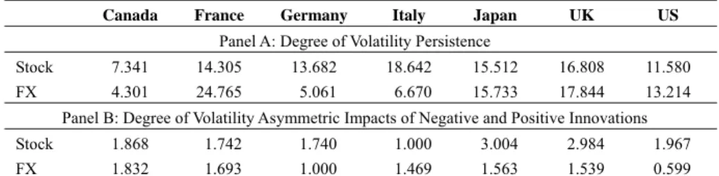
3.2 Volatility Persistence and Asymmetric Volatility Spillover Effect

From Panel A of Table 4, the volatility persistence, measured by γ , of stock i prices and exchange rates is common for all the G-7 countries. The volatility shocks in the stock and foreign exchange markets lasted for 14 and 13 weeks, respectively, on average (based on the half-life of a shock, defined as ln(0.5)/ln(γ ). In Panel B i)

of table 4, the asymmetric impacts of positive and negative innovations are shown. Since the δ are not significant for the exchange rate of Germany and the stock i price of Italy, there is no difference between negative and positive innovations for the respective markets. Nevertheless, asymmetric effects exist for innovations for most series. For example, negative innovations of stock prices in Japan and the UK have impacts on conditional volatility three times larger than positive innovations.

Table 4. Impacts of Innovations on Volatility from the Multivariate EGARCH Model Canada France Germany Italy Japan UK US

Panel A: Degree of Volatility Persistence

Stock 7.341 14.305 13.682 18.642 15.512 16.808 11.580

FX 4.301 24.765 5.061 6.670 15.733 17.844 13.214

Panel B: Degree of Volatility Asymmetric Impacts of Negative and Positive Innovations

Stock 1.868 1.742 1.740 1.000 3.004 2.984 1.967

FX 1.832 1.693 1.000 1.469 1.563 1.539 0.599

Note: Entries in Panel A denote the degree of volatility persistence, based on the half-life of a shock (defined as ln(0.5)/ln(γi)). Entries in Panel B denote the number of times that negative innovations increase volatility more than that of positive innovations, which is defined as |−1+δj|/(1+δj).

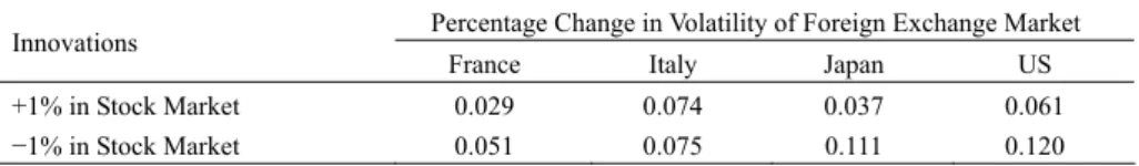
Moreover, based on the estimations of the multivariate EGARCH model, we perform a simulation on the different impacts of good and bad news on the cross-market volatility. The results are presented in Table 5. The total impact of spillover effects from market j to market i is measured by αi j, (1+δj) for a 1%

positive innovation and αi,j|−1+δj| for a 1% negative innovation. For example, a

−1% (1%) innovation in the France, Italy, Japan, and US stock markets increased

volatilities by 0.051% (0.029%), 0.075% (0.074%), 0.111% (0.037%), and 0.120% (0.061%) in the exchange rates for the next week. The negative shocks in the stock markets have greater impacts on the future volatilities for the exchange markets.

Hence, the two markets have both linear and non-linear short-term relationships and they are also linked together through the second moments.

Table 5. Total Impacts of Innovations (Stock Price) on Volatility (Exchange Rate) from the Multivariate Model

Percentage Change in Volatility of Foreign Exchange Market Innovations

France Italy Japan US

+1% in Stock Market 0.029 0.074 0.037 0.061

−1% in Stock Market 0.051 0.075 0.111 0.120

Note: Entries represent the total impact of innovations of stock price on exchange rate, which is defined as )αi,j(1+δj for a positive 1% innovation and αi,j|−1+δj| for a negative 1% innovation.

4. Summary and Concluding Remarks

The paper explores the intertemporal interaction between stock prices and exchange rates for the G-7 countries. The empirical methodology used is the multivariate extension of the EGARCH model, which is capable of capturing potential asymmetries in the volatility transmission mechanism. In particular, we test for mean and volatility spillovers from one market to another and search for evidence of asymmetry; that is, whether negative shocks originating in a stock market (foreign exchange market) exert more or less impact on the foreign exchange market (stock market) than a positive shock of equal magnitude. Evidence shows that movements of stock prices will affect future exchange rate movements, but changes in exchange rates have less direct impact on future changes of stock prices. Also, the results point out significant volatility spillovers and/or asymmetric effects from the stock market to the foreign exchange market for France, Italy, Japan, and the US. Overall, the empirical evidence suggests that there is information flow (transmission) between the two markets and that the two markets are integrated. The stock markets play a relatively more important role than foreign exchange markets in the first and second moment interactions and spillovers. Accordingly, financial managers can obtain greater insight into the management of their international portfolios affected by the two variables. This should be particularly important to international investors and managers when devising hedging and diversification strategies for their portfolios.

References

Aggarwal, R., (1981), “Exchange Rates and Stock Prices: A Study of the US Capital Markets under Floating Exchange Rates,” Akron Business and Economic

Review, 12, 7-12.

Ajayi, R. A. and M. Mougoue, (1996), “On the Dynamic Relation between Stock Prices and Exchange Rates,” Journal of Financial Research, 19(2), 193-207. Ajayi, R. A., J. Friedman, and S. M. Mehdian, (1998), “On the Relationship between

Finance Journal, 9(2), 241-251.

Bahmani-Oskooee, M. and A. Sohrabian, (1992), “Stock Prices and the Effective Exchange Rate of the Dollar,” Applied Economics, 24(4), 459-464.

Berndt, E. K, B. H. Hall, R. E. Hall, and J. A. Hausman, (1974), “Estimation and Inference in Nonlinear Structural Models,” Annals of Economic and Social

Measurement, 4, 653-65.

Bollerslev, T., (1990), “Modelling the Coherence in Short-Run Nominal Exchange Rates: A Multivariate Generalized ARCH Model,” Review of Economics and

Statistics, 72(3), 498-505.

Bollerslev, T., R. Y. Chou, and K. F. Kroner, (1992), “ARCH Modeling in Finance: A Review of the Theory and Empirical Evidence,” Journal of Econometrics, 52 (1/2), 5-60.

Bollerslev, T. and J. M. Wooldridge, (1992), “Quasi-Maximum Likelihood Estimation and Inference in Dynamic Models with Time-Varying Covariances,”

Econometric Reviews, 11(2), 143-72.

Branson, W. H., (1983), “Macroeconomic Determinants of Real Exchange Risk,” in

Managing Foreign Exchange Risk, R. J. Herring ed., Cambridge: Cambridge

University Press.

Dornbusch, R. and S. Fischer, (1980), “Exchange Rates and the Current Account,”

American Economic Review, 70(5), 960-971.

Engle, R. F., (1982), “Autoregressive Conditional Heteroscedasticity with Estimates of the Variance of United Kingdom Inflations,” Econometrica, 50(4), 987-1008. Engle, R. F. and C. W. J. Granger, (1987), “Co-Integration and Error Correction:

Representation, Estimation and Testing,” Econometrica, 55(2), 251-276. Engle, R. F. and V. K. Ng, (1993), “Measuring and Testing the Impact of News on

Volatility,” Journal of Finance, 48(5), 1749-1778.

Frankel, J. A., (1983), “Monetary and Portfolio-Balance Models of Exchange Rate Determination,” in Economic Interdependence and Flexible Exchange Rates, J. S. Bhandari and B. H. Putnam eds., Cambridge: MIT Press.

Chiang, T. C., S.-Y. Yang, and T.-S. Wang, (2000), “Stock Return and Exchange Rate Risk: Evidence from Asian Stock Markets Based on a Bivariate GARCH Model,” International Journal of Business, 5(2), 97-117.

Chiang, T. C. and S.-Y. Yang, (2003), “Foreign Exchange Risk Premiums and Time-Varying Equity Market Risks,” International Journal of Risk Assessment

& Management, 4(4), 310-331.

Gavin, M., (1989), “The Stock Market and Exchange Rate Dynamics,” Journal of

International Money and Finance, 8(2), 181-200.

Granger, C. W. J., B.-N. Huang, and C.-W. Yang, (2000), “A Bivariate Causality between Stock Prices and Exchange Rates: Evidence from Recent Asian Flu,”

Quarterly Review of Economics and Finance, 40(3), 337-354.

Hamao, Y., R. W. Masulis, and V. Ng, (1990), “Correlations in Price Changes and Volatility across International Stock Markets,” Review of Financial Studies, 3(2), 281-308.

Johansen, S., (1988), “Statistical Analysis of Cointegration Vectors,” Journal of

Economic Dynamics and Control, 12, 231-254.

Koutmos, G. and G. G. Booth, (1995), “Asymmetric Volatility Transmission in International Stock Markets,” Journal of International Money and Finance, 14(6), 747-762.

Laopodis, N. T., (1998), “Asymmetric Volatility Spillovers in Deutsche Mark Exchange Rates,” Journal of Multinational Financial Management, 8(4), 413-430.

Lee, T.-H. and Y. Tse, (1996), “Cointegration Tests with Conditional Heteroskedasticity,” Journal of Econometrics, 73(2), 401-410.

Ma, C. K. and G. W. Kao, (1990), “On Exchange Rate Changes and Stock Price Reactions,” Journal of Business Finance and Accounting, 17(3), 441-450. Nelson, D. B., (1991), “Conditional Heteroskedasticity in Asset Returns: A New

Approach,” Econometrica, 59(2), 347-370.

Nieh, C.-C. and C.-F. Lee, (2001), “Dynamic Relationships between Stock Prices and Exchange Rates for G-7 Countries,” Quarterly Review of Economics and

Finance, 41(4), 477-490.

Phillips, P. C. B. and P. Perron, (1988), “Testing for a Unit Root in Time Series Regressions,” Biometrika, 65, 335-346.

So, R. W., (2001), “Price and Volatility Spillovers between Interest Rate and Exchange Value of the US Dollar,” Global Finance Journal, 12(1), 95-107. Soenen, L. and E. Hennigar, (1988), “An Analysis of Exchange Rates and Stock

Prices: The US Experience between 1980 and 1986,” Akron Business and

Economic Review, 19, 7-16.

Solnik, B., (1987), “Using Financial Prices to Test Exchange Rate Models: A Note,”