國 立 交 通 大 學
多媒體工程研究所
碩 士 論 文
基於 Gram‐Schmidt 正交化的 MPEG Surround
降 混 音 器 與 去 相 關 器 之 設 計
Gram‐Schmidt‐based Downmixer and Decorrelator in the
MPEG Surround Coding
研 究 生:陳德沛
指導教授:蕭旭峯
教授
劉啟民
教授
中 華 民 國 九 十 九 年 八 月
基於
Gram-Schmidt 正交化的 MPEG Surround 降混音器與去相關器之
設計
Gram-Schmidt-based Downmixer and Decorrelator in the MPEG
Surround Coding
研 究 生:陳德沛
Student: Der-Pei Chen
指導教授:蕭旭峯
Advisor: Dr. Hsu-Feng Hsiao
劉啟民 Dr.
Chi-Min
Liu
國 立 交 通 大 學
多 媒 體 工 程 研 究 所
碩 士 論 文
A Thesis
Submitted to Institute of Multimedia Engineering College of Computer Science
National Chiao Tung University in partial Fulfillment of the Requirements
for the Degree of Master
in
Computer Science August 2010
Hsinchu, Taiwan, Republic of China
基於 Gram‐Schmidt 正交化的 MPEG Surround 降混音器
與去相關器之設計
學生:陳德沛 指導教授:蕭旭峯 博士 劉啟民 博士 國立交通大學多媒體工程研究所碩士班中文論文摘要
MPEG Surround 乃一項低位元率多聲道音訊壓縮標準。其壓縮的原理是透過 降混音(down‐mix)處理將多聲道訊號耦合成雙聲或單聲道訊號,並計算出聲源定 位的空間參數(spatial parameter),來達到減少聲道數與紀錄聲場之目的。解碼端 透過去相關器產生的去相關訊號(decorrelated signal),並根據空間參數進行升混 音(up‐mix)處理來重建聲源定位與空間寬廣度的環繞效果。因此,編碼端如何將 多聲道耦合成雙聲或單聲道訊號,與去相關訊號的生成,將影響重建聲音的品質。 此篇論文,使用 Gram‐Schmidt 正交化的概念,改進去相關器與二轉一降混 音模組的運作方式。方法的改進效果將透過升混音後訊號與原始訊號的聲道間能 量差與相關性差值變化,及 ODG(Objective Difference Grade)客觀量測與 MUSHRA 主觀測試來驗證。
Gram‐Schmidt‐based Downmixer and Decorrelator in
the MPEG Surround Coding
Student:Der‐Pei Chen Advisor:Dr. Hsu‐Feng Hsiao Dr. Chi‐Min Liu Institute of Multimedia and Engineering College of Computer Science National Chiao Tung UniversityAbstract
MPEG Surround (MPS) coding is an efficient method for multichannel audio coding. In an MPS encoder, downmixing from multichannel signals into a less number of channels is an efficient way to achieve high compression rate. In decoder, an upmixing module combining with the decorrelator is the key module to reconstruct the multichannel signals. This thesis considers the design of the downmixer and the decorrelator with the assistance of the Gram‐Schmidt orthogonal process. The performance of the proposed downmixer and decorrelator is verified through the differences of Channel Level Difference (CLD) and Inter‐Channel Coherence (ICC) between the upmixed signals and the original signals. Also, the objective and subjective quality measurements are conducted.
Acknowledgement
I would like to express my sincere gratitude to my advisor, Prof. Hsu‐Feng Hsiao. His wide knowledge has broadened my horizon on the field of Computer Science and his logical thinking shows me the way to do better research. Also, his understanding, encouraging, and personal guidance have provided a solid foundation for the present thesis.I appreciate Prof. Chi‐Min Liu for his valuable advice. His suggestions and discussions during the weekly meeting are always been helpful for this study. I am grateful to Mr. Han‐Wen Hsu because he gave me a lot of inspirations when I bottlenecked on my research. If I did not have his advice or help, I might have much more hard time than I have already experienced. I am thankful to the labmates or schoolmates I met during my graduate school life at National Chiao Tung University, especially Mr. Yun‐Hsiu Tung. They make my life full of laughter and give me a hand when I am in need of help.
Finally, I owe my loving thanks to my parents, Mr. Yow‐Shin Chen and Ms. Hsia‐Hua Yu. I couldn’t have become what I am right now without their love and care. Therefore, I would like to dedicate my thesis to them.
Part of this work has been published at 128th Convention of Audio Engineering Society. This work is supported by the National Science Council under the contract numbers NSC98‐2221‐E‐009‐093 and NSC98‐2221‐E‐009‐120, which are gratefully acknowledged.
August 2010
Contents
中文論文摘要 ... iii Abstract ... iv Acknowledgement ... v Chapter 1 Introduction ... 1 Chapter 2 Backgrounds ... 4 2.1 Spatial Audio Coding ... 4 2.2 MPEG Surround ... 5 Chapter 3 The Objectives of MPS Coding ... 14 Chapter 4 Design of Downmixer and Decorrelator based on Gram‐Schmidt Orthogonal Process ... 17 4.1 Decorrelator Issue in Decoder ... 17 4.2 Downmixer Issue in Encoder ... 18 4.3 Gram‐Schmidt Orthogonalization Process ... 19 4.4 The GS‐based Decorrelator ... 20 4.5 The GS‐based Downmixer ... 23 Chapter 5 Experiments and Results ... 28 5.1 MPEG Surround Reference Software ... 28 5.2 Test tracks ... 28 5.3 Quality Measurements ... 30 5.4 Proposed Method Verification ... 31 5.5 Waveform Example ... 34 5.6 Spectrogram Example ... 34 5.7 Results of Objective Quality Measure ... 37 5.8 Results of Subjective Quality Measure ... 44 Chapter 6 Conclusion and Future Work ... 45 References ... 46Figure List
Figure 1 MPEG Surround Encoder (5151) ... 2 Figure 2 MPEG Surround Decoder (5151) ... 2 Figure 3 Multichannel encoder and decoder according to spatial audio coding concept [2] ... 4 Figure 4 Structure of the time‐frequency transformation with its inversion ... 6 Figure 5 A MPS frame with two parameter sets of a parameter band ... 7 Figure 6 Diagram of the original decorrelator on hybrid QMF domain signals ... 9 Figure 7 Tree configurations for mono downmix [2] ... 13 Figure 8 Preferred tree configuration for stereo downmix [2] ... 13 Figure 9 The first two steps of Gram‐Schmidt process ... 19 Figure 10 Flowchart of the proposed method to generate proper decorrelated signals . 20 Figure 11 Illustration of the orthogonal process in the GS‐based decorrelator ... 21 Figure 12 Flowchart of the proposed downmix method ... 24 Figure 13 Spectrogram of unprocessed sm01.wav ... 25 Figure 14 Illustration of the orthogonal process in the GS‐based downmixer ... 25 Figure 15 Parameter difference percentage before and after the upmix procedure ... 32 Figure 16 Energy ratio between the original inputs and upmixed outputs ... 32 Figure 17 ODGs for stereo sequences by using the same parameter ... 33 Figure 18 ODGs for stereo sequences by using the original interpolation on upmix coefficients ... 33 Figure 19 Waveform of original unprocessed es03.wav ... 34 Figure 20 Waveform of es03.wav by the CODEC in standard ... 35 Figure 21 Waveform of es03.wav based on GS‐based decorrelator and downmixer ... 35 Figure 22 Spectrogram of original unprocessed sm02.wav ... 36 Figure 23 Spectrogram of sm02.wav by the CODEC in standard ... 36 Figure 24 Spectrogram of sm02.wav based on GS‐based decorrelator and downmixer .. 37Figure 25 ODGs for stereo sequences by using 5151 tree structure ... 39 Figure 26 ODGs for MPEG surround sequences by using 5151 tree structure ... 40 Figure 27 ODGs for MPEG surround sequences by using 525 tree structure ... 40 Figure 28 ODGs for complex sound category from extracted audio (5151) ... 41 Figure 29 ODGs for natural vocal category from extracted audio (5151) ... 41 Figure 30 Waveform of original unprocessed L and R of Friends.wav ... 42 Figure 31 Waveform of L and R of Friends.wav by the CODEC in standard ... 42 Figure 32 Waveform of L and R of Friends.wav based on GS‐based methods ... 43 Figure 33 ODGs for MPEG surround sequences by using different CODEC combinations 43 Figure 34 MUSHRA test on stereo tracks ... 44
Table List
Table 1 ODG improvements of different combinations for GS‐based decorrelator ... 23 Table 2 ODG improvements on different strategies of projection ... 24 Table 3 ODG improvements of different reduction method for GS‐based downmixer 27 Table 4 The twelve tracks recommended by MPEG [4][17] ... 29 Table 5 Detail information of the equipments ... 30 Table 6 Energy ratios for sc02.wav ... 31 Table 7 Improvements of the surround tracks under different erasure (5151) ... 38 Table 8 Information about the extracted DVD audio ... 39Chapter 1 Introduction
In real world, sound could be from anywhere around us. The psycho‐based listening perception gives us the ability to locate the actual position of the sound in 3D world. Therefore, lots of applications, such as multi‐sound tracks movies or multi‐channel DVDs, take advantage of this human perceptual feeling and give us the illusion that we are in the environment made by the creator. Since every channel has different, or slightly different, content to playback, if we treat them separately, that would require a large amount of memory spaces and make it less possible for applications. Fortunately, ISO/IEC provides a solution to deal with multichannel audio coding, called MPEG Surround (MPS).
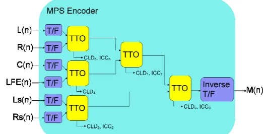
MPS [1]‐[3] is standardized to exploit the correlation among audio channels to achieve high coding efficiency for multi‐channel audio. The concept of MPS is to combine the multichannel signals into a stereo/mono downmixed signal with the spatial parameters including Channel Level Difference (CLD) and the Inter‐Channel Coherence (ICC). The decoder then uses the stereo/mono downmixed signal and the spatial parameters to reconstruct the multichannel signals. There are two key modules affecting the reconstructed audio quality. The first one is the Two‐To‐One (TTO) downmixer, which combines the stereo audio into mono signal and is illustrated in Figure 1. The other is the decorrelator, which generates the “pseudo‐audio” channels for upmixer and is illustrated as the yellow box with “D” in the MPS Decoder shown in Figure 2. This thesis considers the design issues of the TTO downmixer and decorrelator and proposes the novel algorithms for the two critical modules.
Figure 1 MPEG Surround Encoder (5151)
Figure 2 MPEG Surround Decoder (5151)
In MPS decoder, the upmix process is conducted based on the downmixed signals and the decorrelated signals, which are generated by feeding the downmixed signals into a cascade of all‐pass filters. The uncorrelation between the decorrelated signal and the downmixed signal are necessary to reconstruct the audio signals preserving the CLD and ICC of the original signals. However, we will show that the decorrelation cannot be achieved by
the current decorrelator in MPS. This thesis proposes a novel decorrelator based on the GS (Gram‐Schmidt) orthogonalization process which decomposes a non‐ideal decorrelated signal into a correlated component and an uncorrelated component with respect to the downmixed signal. Then the correlated component is turned to be another uncorrelated part by changing the phase of the signal. An adaptive scaling is designed to control the two components to maintain the signal smoothness and the uncorrelation requirement. The proposed decorrelator is compliant to the MPS standard. Experiments show this modification on the decorrelator improves objective difference grade by 0.18 on average.
In an MPS encoder, the TTO downmixer needs to ensure that the energy of the downmixed signal is equal to the sum of the energies of the two input signals so that the upmixed signals in MPS decoder can preserve the energies of the original signals. However, for most of the downmix methods in literature, such as the direct summation of the input signals, the downmixed energy cannot be kept controlled. One straightforward approach is to scale the downmixed signals to fit the energy, but unexpected artifacts might arise due to the possible amplification of the noise. This thesis proposes the GS‐based TTO downmixer which can achieve the equality of energies with consideration to the risk and compliant to MPS standard.
This thesis is organized as follows. Chapter 2 provides an overview of the fundamental components related to the main goal of this thesis in MPEG Surround. Chapter 3 demonstrates that three upmix objectives can be achieved by keeping the desired properties on the TTO downmixer and decorrelator. The problem definition and the proposed solutions are presented in Chapter 4, and the experiments are conducted in Chapter 5. Chapter 6 concludes the thesis.
Chapter 2 Backgrounds
MPEG Surround is under the concept of spatial audio coding, so we would introduce the spatial audio coding first and then go through the components, which is related to the goal of this thesis, in MPEG Surround.2.1 Spatial Audio Coding
The concept of spatial audio coding as employed in MPEG Surround standard is shown in Figure 3. A multi‐channel input is converted to a mono/stereo downmixed signal by a MPEG Surround encoder. The properties of the original input signals which might be lost by downmixing are captured and transmitted through a spatial parameter bit stream. The downmixed signal is process by a legacy downmix encoder. The multiplexer combines the downmixed signal from legacy downmix encoder with the spatial parameter bit stream to one output, which would be the input of the decoder side.After the encoded signal is fed into the decoder shown in Figure 3, demultiplexer separates the downmixed signal and spatial parameter bit stream. The downmixed signal is decoded by the legacy downmix decoder and then is upmixed according to transmitted spatial parameters by MPEG Surround decoder.
2.2 MPEG Surround
Though Figure 1 and Figure 2 only show one of the coding tree structures provided by MPEG Surround, the components inside the tree structures are the same. Therefore, the introductions for each component are needed for the background knowledge.
Time/Frequency Transformation
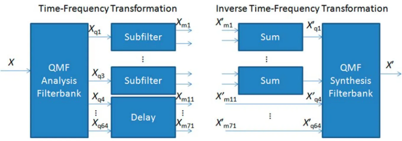
The applied filterbank is a hybrid complex‐modulated quadrature mirror filterbank (QMF). As shown in Figure 1 and Figure 2, the input signals of the encoder and decoder are passed into time/frequency analysis filterbank, which is composed by a QMF analysis filterbank, subfilters and a delay shown in the left panel of Figure 4. The signals are first fed into the QMF analysis filterbank. Since each subband of QMF analysis filterbank has the same bandwidth, the frequency resolution of QMF analysis filterbank cannot response the sense of hearing model in which the lower frequency part requires higher resolution. Therefore, subfilters are used to provide non‐uniform resolution in low frequency and the high frequency part is delayed by the delay module. In Figure 4, the input signal X is fed into the QMF analysis filterbank and turned to be the 64 QMF subband signal, Xqi with 0 ≤ i ≤ 64.
Then the 64 QMF subbands would be splitted to 71 hybrid subbands, Xmj with 0 ≤ j ≤ 71.
While calculating the spatial parameters at the mixing boxes, the 71 hybrid subbands are rearranged to 28 parameter bands, which is the basic unit of MPS, at most. The inverse time/frequency transformation is combined by the sum modules and a QMF synthesis filterbank, shown in the right panel of Figure 4. The modules of sum and QMF synthesis filterbank are corresponding to subfilters and QMF analysis filterbank respectively. Since the filterbank has the same structure as the one applied in Parametric Stereo, detailed introduction and information can be found in [2]‐ [4].
Figure 4 Structure of the time‐frequency transformation with its inversion
Framing
There are some restrictions for time resolution. There are 32 time slots in one frame with at most 8 parameter sets, which are the time slots that keep the calculated spatial parameters. The calculated parameter sets can be places at any time slot by variable framing or the time slots with equal distance by fixed framing. No matter which framing is used, at least one set of parameters are placed in the last time slot of a frame. The time slots that do not have the spatial parameters are then interpolated on the Ra matrix coefficients, which
would be introduced in the next subsection.
Figure 5 illustrates a frame example with two parameter sets of a parameter band. According to the previous paragraph in this subsection, each column indicates a time slot; the columns with gray grounding are the time slot with spatial parameters; the red line indicates the matrix coefficient value; the bold solid line indicates the frame borders; and the blue line illustrates the interpolation of matrix coefficients.
Figure 5 A MPS frame with two parameter sets of a parameter band
Elementary Building Blocks
The common coding blocks for MPEG Surround are One‐To‐Two (OTT) and Two‐To‐Three (TTT) at the decoder side, and the corresponding blocks used on the encoder side are Two‐To‐One (TTO) and Reverse TTT (R‐TTT).
z Encoder
TTO coverts a stereo input signal to a mono signal, combined with parameter extraction which represents the spatial parameters between the respective input signals. Since [1] does not detailed specified how to realize downmixing for encoder, we reference the MPS reference software provided by MPEG [5] and know that the downmixing is realized by the direct summation of the input signals as ] [ ] [ ] [n X1, n X2, n Ym = m + m , (1)
where X1,m and X2,m denotes the input signals on the hybrid subband m; Ym denotes the
output signal; n represents the time slot index.
In the appendix of [1], the power ratio of corresponding time/frequency tiles of the input signals, which would be denoted as “Channel Level Difference” or CLD, is defined as
⎟⎟ ⎟ ⎟ ⎟ ⎠ ⎞ ⎜⎜ ⎜ ⎜ ⎜ ⎝ ⎛ =
∑ ∑
∑ ∑
= − = ∗ = − = ∗ + + 31 0 1 , 2 , 2 31 0 1 , 1 , 1 10 1 1 ] [ ] [ ] [ ] [ log 10 n m m m m m n m m m m m b b b b n X n X n X n X CLD , (2) where mb is the hybrid subband boundaries of the bth parameter band.Also, a similarity measure of the corresponding time/frequency tiles of the input signals, which would be denoted as “Inter‐Channel Correlation” or ICC, is given by the cross correlation as ⎪ ⎪ ⎭ ⎪ ⎪ ⎬ ⎫ ⎪ ⎪ ⎩ ⎪ ⎪ ⎨ ⎧ =
∑ ∑
∑ ∑
∑ ∑
= − = ∗ = − = ∗ = − = ∗ + + + 31 0 1 , 2 , 2 31 0 1 , 1 , 1 31 0 1 , 2 , 1 1 1 1 ] [ ] [ ] [ ] [ ] [ ] [ Re n m m m m m n m m m m m n m m m m m b b b b b b n X n X n X n X n X n X ICC . (3)z Decoder
There are two components in an OTT. The first one is the decorrelator and the other is the Ra upmix matrix. In literature, there are many decorrelation methods [6]‐[12]. In [7], decorrelation works on simple nonlinear functions, which is simple in computations. [8] uses interleaving comb filters and frequency shifts to realize decorrelation. [9] and [10] uses time‐varying all‐pass filters. Boueri et al. [11] proposes a new random time‐shifting method on critical band to lower the cross‐correlation. A Karhunen–Loève transform based method is also mentioned in [12] for decorrelation. Despite the fact there are many approaches for decorrelation, only the approach used for MPS decorrelator is discussed in this thesis.Decorrelators are used to generate an uncorrelated signal from the input to simulate the missing channel(s) information for the upmix matrix operations. They are realized by
comprising a delay, a lattice all‐pass filter, and an energy adjustment stage shown in Figure 6. The configurations for the delay and all‐pass filter are controlled by the decorrelator configuration transmitted from encoder. For MPEG Surround, the OTT and prediction‐mode TTT have one decorrelator in both them.
Figure 6 Diagram of the original decorrelator on hybrid QMF domain signals
Let us detailed introduce how the original decorrelator operates. The delayed hybrid subband domain samples Ddelay[n] m are obtained as ⎪ ⎪ ⎩ ⎪ ⎪ ⎨ ⎧ − ∈ − − ∈ − − ∈ − − ∈ − = 71 30 , ] 1 [ 29 21 , ] 2 [ 20 8 , ] 7 [ 7 0 , ] 8 [ ] [ m n M m n M m n M m n M n D m m m m delay m , (4) where Mm[n] for n < 0 contains the buffered values of the last frame at position 32 – n. Then
the delayed hybrid subband domain samples Dmfilt[n] are filters as
⎟ ⎠ ⎞ ⎜ ⎝ ⎛ − ⋅ − − ⋅ ⋅ =
∑
∑
= = S s filt m m S s delay m m m filt m b s D n a s D n a n D 1 0 ] 1 [ ] [ ] 1 [ ] [ ] 0 [ 1 ] [ , (5) where S is the length of the lattice coefficient vector s[n] and the filter coefficients am[n] and bm[n] are derived from the lattice coefficient vector s[n], which is well‐defined in the Section 6.6 in [1].After the Dfilt[n]
m have been obtained for 0 ≤ n < 32, the following energy adjustment
procedure is applied. The powers per parameter band k of the input samples EM[n]
k and the filtered samples ED[n] k are calculated as ( )
∑
= ∈ ∀ = k m m m M k n M n E κ 2 ] [ ] [ , (6) ( )∑
= ∈ ∀ = k m m filt m D k n D n E κ 2 ] [ ] [ , (7) with κ(m) defines in Table A.31 in [1], which is a lookup table for hybridband to parameter band. Then, low‐pass filtering on the powers is applied as ] [ ) 1 ( ] 1 [ ] [ , , n E n E n E M k Smooth M k Smooth M k =α⋅ − + −α ⋅ , (8) ] [ ) 1 ( ] 1 [ ] [ , , n E n E n E D k Smooth D k Smooth D k =α⋅ − + −α ⋅ , (9)with α = 0.8. For the first slot of the first frame both EM,Smooth[n−1]
k and ] 1 [ , n− EDSmooth k with n = 0 are initialized as zero vector. For the first slots of all other frames, both EM,Smooth[n−1] k and ED,Smooth[n−1] k with n = 0 are set to the value of [ ] , n EMSmooth k and ] [ , n EDSmooth k of the previous frame at n = 31. The energy‐shaping gain vector is calculated as ⎪ ⎪ ⎪ ⎪ ⎩ ⎪ ⎪ ⎪ ⎪ ⎨ ⎧ > ⎟ ⎟ ⎠ ⎞ ⎜ ⎜ ⎝ ⎛ + > + = otherwise n E n E n E n E n E n E n E n E n g MSmooth k Smooth D k Smooth D k Smooth M k Smooth M k Smooth D k Smooth D k Smooth M k k , 1 ] [ ] [ , 2 , ] [ ] [ min ] [ ] [ , ] [ ] [ ] [ , , , , , , , , γ ε γ γ ε γ , (10)
with γ = 1.5 and ε = 1e ‐9. Finally, the decorrelator outputs are constructed as ] [ ] [ ] [n g ( ) n D n D filt m m m = κ ⋅ . (11)
The OTT matrix operation in Figure 2 is represented as ⎥ ⎦ ⎤ ⎢ ⎣ ⎡ = ⎥ ⎦ ⎤ ⎢ ⎣ ⎡ ] [ ] [ ] [ ] [ , ' , 2 ' , 1 n D n M R n X n X m m m n a m m , (12)
where Mm[n] is the downmixed hybrid subband signal; Dm[n] is the output signal of the
decorrelator for Mm[n]; X’1,m[n] and X’2,m[n] are the upmixed signals. According to the
parameters ICC and CLD, MPS standard specifies Ra as
(
)
(
)
(
)
(
)
⎥⎦⎤ ⎢ ⎣ ⎡ + − + − + + = ⎥ ⎦ ⎤ ⎢ ⎣ ⎡ = β α λ β α λ β α λ β α λ sin cos sin cos 22 21 12 11 2 2 1 1 , H H H H Rlm a , (13) where(
ICC)
arccos 2 1 = α , (14)( )
⎟⎟ ⎠ ⎞ ⎜⎜ ⎝ ⎛ + − = α λ λ λ λ β tan arctan 1 2 1 2 , (15) 10 / 10 / 1 10 1 10 CLD CLD + = λ , (16) 10 / 2 10 1 1 CLD + = λ , (17) and( )
(
( )
)
( )
( )
(
( )
)
( )
( )
⎪⎩ ⎪ ⎨ ⎧ < ≤ ≤ ≤ − − + = ≤ ≤ − + = − − L l l n l R l n l n R l l n R l n l n R R m l a m l a m a m l a m n a 1 , 1 , , 1 , 0 , 0 , , 1 , , 1 , , 1 , , t t t α α α α (18) for 0 ≤ l < L where( )
( )
( )
( ) ( )
⎪ ⎪ ⎩ ⎪⎪ ⎨ ⎧ ∀ − − − − = ∀ + + = otherwise l n l l l n l n l n l n : ; , 1 t t 1 t 0 ; , 1 t 1 , α , (19) and where L denotes the number of parameter sets, and t(l) denotes the time slot of parameter set l.The matrix operations used for TTT have different modes, prediction mode and energy reconstruction mode, which are fully introduced in [3].
Tree Structures
The common coding blocks for MPEG Surround mentioned in the previous subsection can be cascaded to form the desired spatial coding tree, depending on the specified numbers of inputs and outputs, and additional features. Though MPS can deal with the sequences with 7.1 channels, only the most common tree structures for 5.1 channel input would be described in this subsection.
The first type of tree structures for 5.1 channel input is 5151 and 5152, which supports a mono downmixed signal. Both 5151 and 5152 are shown in Figure 7a and Figure 7b respectively. The six input channels, left front (L), right front (R), left surround (Ls), right surround (Rs), center (C), and low frequency enhancement (LFE) are fed into TTO box pairwisely until a mono downmixed signal is obtained.
To downmix the inputs to the stereo signal, the second type of tree structures is provided, which is commonly known as 525. Figure 8 shows the preferred tree structure for stereo downmix. L and Ls, R and Rs, and C and LFE are processed by R‐OTT box separately and then the outputs of the three TTO boxes are fed into a R‐TTT box to generate a stereo downmixed signal.
To upmix the downmixed signal, the decoding tree structures are the inversion of the encoding one, which would give the most similar results. For detailed information, please refer to [1]‐[3].
Figure 7 Tree configurations for mono downmix [2] Figure 8 Preferred tree configuration for stereo downmix [2] (a) 5151 configuration (b) 5152 configuration
Chapter 3 The Objectives of MPS Coding
In order to let the perceptual feeling of decoded output to be the same as the feeling to the original input, there exist some objectives based on the statistical properties between channels. In this chapter, we introduce the objectives which are set for the upmix matrix in an OTT box and derive how they would be held.
Let Xm be a column vector representing a complex hybrid subband signal Xm[n] in a
processing frame, for n = n0, n0+1,…, n1, i.e., Xm = [Xm[n0], Xm[n0+1], Xm[n0+2]…, Xm[n1]]T,
where superscript T means the transpose operation and n0 = 0 and n1 = 31. An ideal
decorrelator should generate an uncorrelated signal with the same energy of its input, i.e. Re{<Mm, Dm>} = 0 and ||Mm||2 = ||Dm||2, where Re{‧} takes the real part of an input; <‧>
means the inner product and ||‧|| means the vector norm. From (12) to (17), if all the
CLDs and ICCs are the same for the time slot n = n0, n0+1,…, n1, the energy of the upmixed signal X’1,m[n], with an ideal decorrelator, can be derived as ( ) ( ) ( ) ( ) 2 2 1 2 2 2 2 2 1 2 λ , β α β α 2 β α β α λ m m m m m m 1, M D M D M X' ⋅ = ⎟ ⎟ ⎠ ⎞ ⎜ ⎜ ⎝ ⎛ > < + + + + + + ⋅ = } { Re sin cos sin cos . (20) Likewise, the energy of the upmixed signal X’2,m[n] is reduced to 2 2 2 2 , 2m Mm X' =λ ⋅ . (21) The correlation of the upmixed signals is derived as
(
) (
)
(
) (
)
(
) (
)
(
) (
)
. ) 2 cos( sin sin , cos sin , sin cos cos cos Re } , Re{ 2 2 1 2 2 2 1 2 1 m m m m m m m ,m ,m M D M D D M M X' X' ⋅ ⋅ = ⎪ ⎪ ⎭ ⎪ ⎪ ⎬ ⎫ ⎪ ⎪ ⎩ ⎪ ⎪ ⎨ ⎧ ⋅ + − + + > < ⋅ + − + + > < ⋅ + − + + ⋅ + − + ⋅ = > < α λ λ β α β α β α β α β α β α β α β α λ λ . (22)Objective I—
The correlations among the upmixed signals from multiple channels are the same as the correlations of the original signals. According to the definition of the ICC parameter in the MPS standard, the ICC value of the two upmixed signals in a parameter band is calculated as ⎟ ⎟ ⎟ ⎟ ⎟ ⎠ ⎞ ⎜ ⎜ ⎜ ⎜ ⎜ ⎝ ⎛ ⋅ > < = Φ
∑
∑
∑
− = − = − = + + + 1 2 2 1 2 1 1 2 1 1 1 1 2 1 , Re b b b b b b m m m ,m m m m ,m m m m ,m ,m X X X' X' X' X' , (23) From (20)‐(22), under a ideal decorrelator, (23) can be reduced to ). 2 cos( 2 1 = α ΦX X (24) Comparing (24) with (14) shows that Objective I holds with an ideal decorrelator. Objective II— The power ratios among the upmixed signals from different channels are the same as those of the original audio signals. According to the definition of the CLD parameter in MPS standard, the CLD value of the two upmixed signals in a parameter band is calculated as ⎟⎟ ⎟ ⎟ ⎟ ⎠ ⎞ ⎜⎜ ⎜ ⎜ ⎜ ⎝ ⎛ = Δ∑
∑
− = − = + + 1 2 2 1 2 1 10 1 1 2 1 10log b b b b m m m ,m m m m ,m X X L X' X' . (25) By (20) and (21), with an ideal decorrelator, (25) can be reduced as ⎟ ⎟ ⎠ ⎞ ⎜ ⎜ ⎝ ⎛ = Δ 2 2 2 1 10 log 10 2 1 λ λ X X L . (26) From (16) and (17), this result shows that Objective II holds with an ideal decorrelator.Objective III— The sum of the energies of the upmixed signals from multiple channels must be equal to the energy of the input signals. From (16) to (17) and (20) to (21), the energy of the two upmixed signals in a parameter band is calculated as . 1 2 1 2 2 1 2 1 1 1 1
∑
∑
∑
− = − = − = + + + = + b b b b b b m m m m m m m ,m m m m ,m X' M X' (27)This means that, if the encoder generates an energy‐preserved downmixed signal, Objective III holds with an ideal decorrelator. The above three objectives are held under the circumstances that Re{<Mm, Dm>} = 0 and ||Mm||2 = ||Dm||2 and all the CLDs (2) and ICCs (3) are kept the same for the time slot n = n0, n0+1, …, n1 while doing (12).
Chapter 4 Design of Downmixer and Decorrelator based on
GramSchmidt Orthogonal Process
As shown in the previous chapter, to preserve the objectives of MPS coding, it is essential that a decorrelator generates an uncorrelated signal with the same energy of its input. An energy‐preserved encoder is also important. We would demonstrate the limits of the current decorrelator and encoder, and then propose our methods based on Gram‐Schmidt orthogonal process.
4.1 Decorrelator Issue in Decoder
In this subsection, we analyze the effect of the decorrelator, which is a cascaded all‐pass filters in MPS standard, on the basis of [13]. A general subband signal can be approximated as ] [ ) exp( ] [ 1 0 n N a n j a n x M n k k k + =∑
− =ω
, (28)where the subband signal contains M sinusoid signals and an AWGN component N[n]. The cross power spectral density of x[n] and the output signal y[n] from the all‐pass filters can be derived as ⎥ ⎦ ⎤ ⎢ ⎣ ⎡ − + = =
∑
− = 2 1 0 2 ) ( ) ( ) ( ) ( ) ( N n M k k k XX YX a a D S D S σ ω ω δ ω ω ω ω , (29) where δ(ω) is the Dirac delta function, σ is the variance of the AWGN noise signal N[n], N2 and D(ω) is the frequency response of the decorrelator. The cross correlation at zero lag is calculated as⎥ ⎦ ⎤ ⎢ ⎣ ⎡ + = ⎥ ⎦ ⎤ ⎢ ⎣ ⎡ − + =
∫
∑
∫
∑
− = − = π π ω ω σ ω π ω σ ω ω δ ω π 2 0 2 1 0 2 2 0 2 1 0 2 ) ( ) ( 2 1 ) ( ) ( 2 1 ] 0 [ d D a D a d a a D R N n M k k k N n M k k k yx (30) We can consider (30) from two extreme cases. If the input signal is noise‐like (ak = 0 for all k), the cross correlation value can be approximated as[ ]
0 ) ( 2 ] 0 [ 2 2 0 2 d a d D a R n N n N yx ≈ π ⋅∫
ω ω = σ ⋅ σ π . (31) where d[0] is the impulse response of the all‐pass filters at n = 0. The value can be controlled to be zero for the all‐pass filters. Hence, the cross correlation value can be zero if the input signal is white. However, if the input signal is purely tonal (an = 0 for all n), the crosscorrelation value is
∑
− = ≈ 1 0 2 ) ( 2 1 ] 0 [ M k k k yx a D Rω
π
. (32) Thus, we can expect that the output signal of the decorrelator can be highly correlated to the original tonal signal. In other words, the effect of the all‐pass filters defined in MPS standard has the decorrelating effect varying with the tonal components in the subband signals.4.2 Downmixer Issue in Encoder
Most of the current downmix methods, such as the direct summation of the input signals, cannot guarantee that the energy of the output is the same as that of the input. This inconsistent makes the energy summation of the decoded output signals different than that of the original input signals. One straightforward way is to directly adjust the downmixed signals, but unexpected artifacts might arise due to the possible amplification of the noise.
4.3 Gram‐Schmidt Orthogonalization Process
Gram‐Schmidt[14][15] is a method to construct an orthonormal basis in a k‐dimensional inner product space. This process takes a finite, linearly independent set {v1, v2, …, vj} for j ≤ k
and generates an orthogonal set {u1, u2, …, uj}.
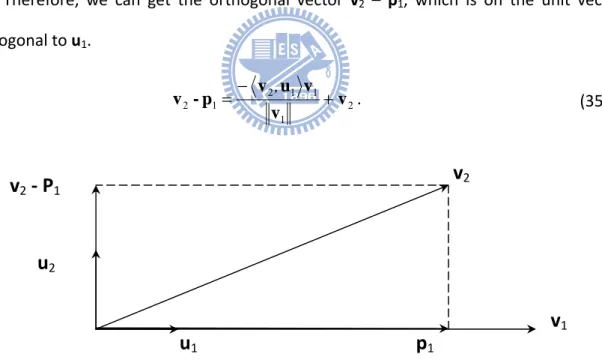
Figure 9 shows the first two steps of Gram‐Schmidt process. We can consider u1 as the normalized vector of v1. 1 1 1 v v u ⎟⎟ ⎠ ⎞ ⎜ ⎜ ⎝ ⎛ = 1 (33)
Let p1 denote the projection of v2 onto v1.
1 1 2
1 v u u
p = , . (34)
Therefore, we can get the orthogonal vector v2 – p1, which is on the unit vector u2
orthogonal to u1. 2 1 1 1 2 1 2 v v v u v p -v = − , + . (35) Figure 9 The first two steps of Gram‐Schmidt process
The idea of Gram‐Schmidt is explained by the first two steps of the process. We can repeat the idea and calculations shown from (33) to (35) to reach the desired k‐dimension inner product space.
v
1u
1u
2v
2p
1v
2‐ P
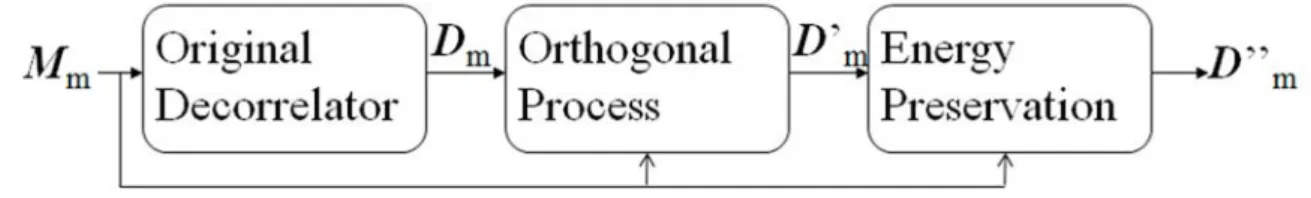
14.4 The GS‐based Decorrelator
To ensure the uncorrelation between the decorrelated signal and the downmixed signal, a Gram‐Schmidt based decorrelator (see Figure 10) is proposed to modify the output signal.
Figure 10 Flowchart of the proposed method to generate proper decorrelated signals
By applying the Gram‐Schmidt orthogonalization process to { Mm , Dm }, Dm can be
decomposed as m m m m m m m m m , V P V M M M M D D =< >⋅ + = 1 + . (36)
Although Vm is uncorrelated to Mm, the projection part of Dm is correlated to Mm, which
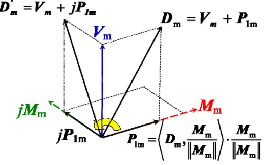
leads to the decorrelation defect. On second thought that the original decorrelator process changes the phase of the signal to realize orthogonality and only the real‐part decorrelation is required, a modified decorrelated vector can be constructed by multiplying scale j, which means another 90∘shift on the signal, to the projection part: m m m m m m m j , V M M M M D D′ = < >⋅ + . (37)
The real part of the inner product of Mm and D’m is given by
(
,)
Re(
,)
0Re < Dm′ Mm > = <Vm Mm > = , (38) and thus we confirm that D’m is uncorrelated to Mm. (see Figure 11)
Figure 11 Illustration of the orthogonal process in the GS‐based decorrelator On the other hand, the energy of D’m is given by 2 2 2 2 m m m m m m , V M M D D D′ = = < > + . (39)
The energy of D’m is not guaranteed to be the same as the energy of Mm since jP1m is
correlated to Vm. Energy adjustment is required to ensure the equality of the energies of the
decorrelated and downmixed signals. From the decoder’s point of view, Mm is transmitted
from the encoder, which can be considered as the signal similar with the original input signals. Therefore, jP1m can be amplified without the risk of other artifacts if the energy of
D’m is less than the energy of Mm. In the opposite case, if the energy of D’m is larger than the
energy of Mm, keeping the same relation of jP1m and Vm which is generated by original
decorrelator, is important since reduction can be consider as a suppression on the component.
We verify our thoughts by different method combinations of increasing or decreasing the energy. The two ways to increase the energy, called Increase A and B, and two ways of decrease the energy, called Reduction A and B, are listed below:
z Increase A: ⎟ ⎟ ⎠ ⎞ ⎜ ⎜ ⎝ ⎛ + ⋅ > < = ′′ m m m m m m m j , V M M M M D D ρ , (40) with m m D M = ρ . (41) z Increase B: m m m m m m m j V M M M M , D D′′= ρ< >⋅ + , (42) with > < − = m m m m m , M M D V M 2 2 ρ . (43) z Reduction A: ⎟ ⎟ ⎠ ⎞ ⎜ ⎜ ⎝ ⎛ + ⋅ > < = ′′ m m m m m m m j , V M M M M D D ρ , (44) with m m D M = ρ . (45) z Reduction B: m m m m m m m V M M M M D D′′ = j< , >⋅ + ρ , (46) with m m m m m D M M V M 2 2 2 , 1 ρ= ⎜⎝⎛ − ⎟⎠⎞ . (47) If ρ in (47) is not in the range of 0 to 1, the surplus energy would be reduced from the projection part only as m m m m m m M M M M D D′′ = jρ< , >⋅ , (48) with
2 1 m m m M M D , ρ= . (49) The best combination is the one using Increase B for increasing energy and Reduction A for decreasing energy, which agrees our primary thought on energy adjustment, after we compare the improvements of averages objective quality measurements (ODG) of different combinations, listed in Table 1. Table 1 ODG improvements of different combinations for GS‐based decorrelator Increase A + Reduction A Increase A + Reduction B Increase B + Reduction A Increase B + Reduction B ODG Improvement 0.04 ‐0.4 0.18 ‐0.28
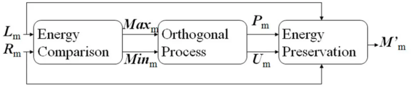
4.5 The GS‐based Downmixer
The advantages of direct summation of the input signals are trivial, but this method does not guarantee that the energy of the output is the same as that of the input. From (1), the energy of Ym can be derived as > < + + = 1,m 2,m 1,m 2,m m X X X X Y 2 2 2 2 , . (50)
If the correlation exists among X1,m and X2,m, the term 2<X1,m, X2,m> exists and the
energy of Ym is not equal to the sum of energies of X1,m and X2,m. Therefore, a Gram‐Schmidt
based downmix method, based on direct summation of the input signals, is proposed. The flowchart of the proposed downmix method is depicted in Figure 12, where Maxm is the
input signal with larger energy, Minm is the input signal with smaller energy, Pm is the sum of
projection part of Minm and Maxm, and Um is the orthogonal part of Minm. Based on the
same idea of GS‐based decorrelator, the Gram‐Schmidt process can be applied to the input vector set {Lm, Rm}.
Combinations Comparison
Figure 12 Flowchart of the proposed downmix method
In the beginning, we simply made Rm as the projection basis and decomposed Lm. For
most of the test sequences, the ODGs improved. However, there were some results of test sequences, like sm01.wav, were even worse than the one processed by the original encoder. After analyzing the spectrogram of sm01.wav shown in Figure 13, we discovered that the choice of the basis to project on is crucial. The right channel has less energy than the left channel, so the Gram‐Schmidt process would decompose the channel with more energy, which might lead to information loss for downmixing. Therefore, the first stage is to compare the energies of two input hybrid subbands and choose the one with larger energy to be the basis of projection. The average improvements for different strategies of projection are listed in Table 2, which is based on the encoder method published in [16]. Table 2 ODG improvements on different strategies of projection Right Channel Channel with More Energy ODG Improvement 0.22 0.3
After comparing the energies of Lm and Rm, let Maxm represents the one with larger
energy and Minm represents the other one.
The second stage (see Figure 14) perform the Gram‐Schmidt process to decompose
Minm as
Proj. Stgy. Comparison
m m m m m m Max U Max Max Min Min =< , > + , (51) where Um is the uncorrelated with respect to the projection basis. Therefore, the downmixed signal Mm can be expressed as m m m m m m m m m , Max U P U Max Max Min Max M = +< > + = + . (52) Figure 13 Spectrogram of unprocessed sm01.wav Figure 14 Illustration of the orthogonal process in the GS‐based downmixer Left Channel Right Channel
The energy of Mm is not guaranteed to be the same as the summation of the energies of
Lm and Rm, which is shown in (50). Energy adjustment is required to ensure the equality of
the energies of the downmixed and inputs signals. If the energy of Mm is less than the
summation of the energies of Lm and Rm, amplifying their same component is a better way
for energy adjustment, which is based on the idea that it is important to keep most of the common component in both inputs. If the energy of Mm is more than the summation of the
energies of Lm and Rm, keeping the different component without losing the same one is
better.
We verify the different method combinations for energy adjustment. The ways for increasing the energy of Mm, called Increase 1 and 2, and decreasing the energy of Mm, called
Reduction 1 and 2, are listed below: z Increase 1: the insufficient energy is adjusted by the entire Mm
(
m m)
m P U M' =ρ + , (53) with 2 2 2 m m m R M L + = ρ . (54) z Increase 2: the insufficient energy is adjusted by Pm m m m P U M' = ρ + , (55) with 2 2 2 2 m m m m R U P L + − = ρ . (56) z Reduction 1: the surplus energy would be reduced from the entire Mm as(
m m)
m P U M' =ρ + , (57) with 2 2 2 m m m R M L + = ρ . (58)m m m P U M' = +ρ , (59) with 2 2 2 2 m m m m R P U L + − = ρ . (60) If ρ in (58) is not in the range of 0 to 1, the surplus energy would be reduced from Pm only as m m P M' = ρ , (61) with 2 2 2 m m m R P L + = ρ . (62)
After comparing with the improvements of average ODGs shown in Table 3, the combination of Increase 2 and Reduction 1 gives the best result, which fits the energy adjustment principle. Table 3 ODG improvements of different reduction method for GS‐based downmixer Increase 1 + Reduction 1 Increase 1 + Reduction 2 Increase 2 + Reduction 1 Increase 2 + Reduction 2 ODG Improvement 0.32 0.3 0.45 0.42 Combinations Comparison
Chapter 5 Experiments and Results
The proposed methods in chapter 4 are implemented on the MPEG Surround reference software and evaluated through the objective and subjective quality tests by plenty of stereo and surround test sequences. In this chapter, we introduce the software, list the test sequences we use, show the differences we observe, and experiment through quality tests in this chapter.
5.1 MPEG Surround Reference Software
The MPEG Surround committee provides a reference software for MPEG Surround [5]. The software is developed in Microsoft Visual Studio environment and is written in the programming language of C. Because the specification defines the MPEG Surround decoding processes, the decoding reference software is supposed to be fully normative with the standard. However, the encoding process is not specified by the standard, so the encoder in the reference software only provides the simplest method that fits the required syntax on the specifications. There are only three downmix tree structures provided: 5151, 5152, and 525. The outputs of the encoder and decoder are not further compressed nor decompressed by any rate control.
5.2 Test tracks
Since the proposed methods are used for the OTT and TTO boxes, creating a stereo condition is also feasible for confirming the effect. We use twelve stereo test tracks recommended by MPEG and listed in Table 4. These tracks include the critical music balancing on the percussion, string, wind instruments, and human vocal. To simplify the effective tree structure to only one pair of TTO and OTT box, the stereo test tracks are extended to six‐channel sequences by padding zeros in the C, Ls, Rs, and LFE channels, which would give the same results conducted by Parametric Stereo. There are also four surround
test tracks from the MPEG.
Table 4 The twelve tracks recommended by MPEG [4][17]
Tracks
Signal Description
Signals Mode Time (sec) Remark
1 es01 Vocal (Suzan Vega) stereo 10 (c)
2 es02 German speech stereo 8 (c)
3 es03 English speech stereo 7 (c)
4 sc01 Trumpet solo and orchestra stereo 10 (b) (d)
5 sc02 Orchestral piece stereo 12 (d)
6 sc03 Contemporary pop music stereo 11 (d)
7 si01 Harpsichord stereo 7 (b)
8 si02 Castanets stereo 7 (a)
9 si03 pitch pipe stereo 27 (b)
10 sm01 Bagpipes stereo 11 (b)
11 sm02 Glockenspiel stereo 10 (a) (b)
12 sm03 Plucked strings stereo 13 (a) (b)
Remark: (a) Transients. (b) Tonal/Harmonic structure. (c) Natural vocal (critical combination of tonal parts and attacks). (d) Complex sound.
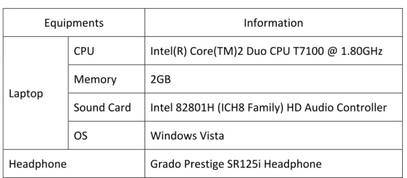
Table 5 Detail information of the equipments Equipments Information Laptop CPU Intel(R) Core(TM)2 Duo CPU T7100 @ 1.80GHz Memory 2GB Sound Card Intel 82801H (ICH8 Family) HD Audio Controller OS Windows Vista Headphone Grado Prestige SR125i Headphone
5.3 Quality Measurements
The objective quality experiments in this thesis are evaluated by EAQUAL (Evaluation of Audio Quality) which simulates the perception by human ears. It is the realization of BS.1387 [18], recommended by ITU Radio Communication Sector. The range of the objective difference grade (ODG) is from -4 to 0 with 0 the best quality. To evaluate the performance of the proposed methods, four kinds of combinations are compared: Original Encoder (OE) + Original Decoder (OD), OE + Modified Decoder (MD), Modified Encoder (ME) + OD, and ME + MD. However, EAQUAL only takes one‐channel or two‐channel inputs. Therefore, after the surround tracks are processed, they are separated into stereo/mono tracks, except LFE, to calculate the ODG.PsyTel Multiple Codec Evaluation Software [19], which follows the test method and impairment scale recommended by ITU‐R BS. 1116 [20], is used for subjective listening test. The system allows blind comparison of multiple audio files. Subjects with proper assessment training could give grades in the range from 1 to 5 with 5 means imperceptible difference. This test includes 12 stereo test sequences. Also, the same laptop and earphone (see Table 5) are provided for all the subjects in the stereo condition.
5.4 Proposed Method Verification
It is obvious that the Ra upmix matrix works on every time slots and dissatisfies the
requirement that all the CLDs and ICCs are the same for the time slot n = n0, n0+1,…, n1. Since
not all the prerequisites are satisfied, the actual three objectives cannot be held.
To verify whether the objectives mentioned in Chapter 3 would be kept under the proposed method, the interpolation method (18) has to be modified as
( )
l l L n R R lm a m n a, = , ,0≤ ≤t ,0≤ < (63)Figure 15 shows the CLD and ICC difference percentage between the transmitted parameters and the ones calculated from the upmixed signals. Figure 16 shows the energy ratio between the original inputs and the upmixed outputs. The energy ratios of MEMD are all close to 100%. The reason for not exactly 100% is that the energy loss caused by time‐frequency transformation after testing the energy ratios before and after the Ra upmix
procedure and the ones from the output and input files. Table 6 shows the energy ratios of the sc02.wav, which losses the most energy in the stereo test sequences. Therefore, both of Figures 15 and 16 tell that using our proposed methods can satisfy the objectives mentioned in Chapter 3. Also, Figure 17 shows after satisfying the objectives, objective quality measurement gives better results for our proposed method.
Table 6 Energy ratios for sc02.wav
Proposed Encoder Proposed Decoder
Hybridband Entire File Hybridband Entire File
sc02.wav 99.6% 100.0% 99.6% 96.1%
We also test the objective quality measurements of the stereo test sequences by using the original Ra interpolation method, showing in Figure 18. The ODGs show our proposed
methods still give better results comparing with the original downmixer and decorrelator. Ratio
Domain Test
Figure 15 Parameter difference percentage before and after the upmix procedure
Figure 17 ODGs for stereo sequences by using the same parameter
5.5 Waveform Example
Figures 19‐21 show the waveform of the frame, which gives the most energy ratio difference by 201.1%, of es03.wav under different circumstances. Figure 20 shows obvious amplification on the waveform by using the original methods. On the contrary, the waveform shown in Figure 21, which is processed by the GS‐based methods, is much similar with Figure 20 with the energy ratio of 100.6% in this frame.
5.6 Spectrogram Example
Figures 22‐24 show the spectrograms of sm02.wav under different circumstances. In Figure 23, the spectrogram by the original methods shows some discontinuities. Also, the energy of each tone decays. On the contrary, in Figure 24, the spectrogram by the GS‐based methods is smoother and preserves the energy. Figure 19 Waveform of original unprocessed es03.wav
Figure 20 Waveform of es03.wav by the CODEC in standard
Figure 21 Waveform of es03.wav based on GS‐based decorrelator and downmixer
Figure 22 Spectrogram of original unprocessed sm02.wav Figure 23 Spectrogram of sm02.wav by the CODEC in standard L Channel R Channel L Channel R Channel
Figure 24 Spectrogram of sm02.wav based on GS‐based decorrelator and downmixer
5.7 Results of Objective Quality Measure
The experiment results for the stereo condition are shown in Figure 25. In Figure 26 and Figure 27, four six‐channel test sequences are conducted based on different coding tree structure. As shown in Figures 25‐27, the proposed methods have improvements over the OE and OD in average. However, the improvement of surround sequences are much less than the ones given by stereo sequences. We erase the content by 2 channels to 4 channels in order to check whether we would get the similar results from the average improvements from the 12 stereo tracks. The corresponding average improvements are listed in Table 7. Even these MPEG four surround tracks are reduced to stereo sequences, the improvement of average ODGs is less than the one from the 12 stereo tracks, which is 0.56 on average. Therefore, these four MPEG surround tracks cannot reflect the benefit of our proposed methods.
L Channel
Table 7 Improvements of the surround tracks under different erasure (5151)
Track Type Surround Track Stereo Track
Erasure None C, and LFE Ls, Rs, C, and LFE None
ODG Improvement 0.05 0.05 0.19 0.56
From the algorithms of the proposed methods, test tracks with high correlations between different channels are the ones that could give better results. To find the appropriate test tracks, we extract the six‐channel audio from DVDs, such as operas, live concerts, and TV series, which are listed in Table 8. We also categorize the extracted audio into two categories: complex sound and natural vocal. The objective quality measurements of these two categories are shown in Figure 28 and Figure 29 with 0.18 and 0.5 ODG improvements on average correspondingly. Though these figures show better results compared with the one from MPEG surround test sequences, we still believe that we could get even better results if the sound tracks of DVD have not been post‐produced. Figures 30‐32 show the waveform of L and R of Friends.wav, which has the greatest improvement on ODG among surround cases. We also notice our proposed methods make the ODG of Ls and Rs of pops.wav worse than the one from the original CODEC by 0.03 under the coding tree structure 5151. Since the energy adjustment for either GS‐based decorrelator or GS‐based downmixer is calculated based on a period of time, we think the problem may be caused by the inconsecutive of the energy adjustment coefficients between two processing periods. We fix this problem preliminary by interpolating the coefficients in the downmixer for the first ten time slots in a processing period and we got positive improvements on ODG of the Ls and Rs of pops.wav. However, this smoothing process causes other surround tracks worse than the one processed by original downmixer, shown in Figure 33. Therefore, this issue is considered as a future work from this thesis.
![Figure 3 Multichannel encoder and decoder according to spatial audio coding concept [2]](https://thumb-ap.123doks.com/thumbv2/9libinfo/8387873.178557/13.892.198.746.863.1048/figure-multichannel-encoder-decoder-according-spatial-coding-concept.webp)

![Table 4 The twelve tracks recommended by MPEG [4][17]](https://thumb-ap.123doks.com/thumbv2/9libinfo/8387873.178557/38.892.119.805.242.895/table-the-twelve-tracks-recommended-by-mpeg.webp)