台灣半導體廠資料包絡法 Malmquist 生產力分析

國 立 交 通 大 學

工業工程與管理學系

碩 士 論 文

台灣半導體廠資料包絡法 Malmquist 生產力分析

DEA Malmquist Productivity Measure:

Taiwanese Semiconductor Companies

研 究 生：王鵬翔

指導教授：劉復華 教授

台灣半導體廠資料包絡法 Malmquist 生產力分析

DEA Malmquist Productivity Measure:

Taiwanese Semiconductor Companies

研 究 生：王鵬翔 Student：Peng-Hsiang Wang 指導教授：劉復華 Advisor：Fuh-Hwa F. Liu 國 立 交 通 大 學 工 業 工 程 與 管 理 學 系 碩 士 論 文 A Thesis

Submitted to Department of Industrial Engineering & Management National Chiao Tung University

in partial Fulfillment of the Requirements for the Degree of Master

In

Industrial Engineering & Management January 2007

Hsinchu, Taiwan, Republic of China

台灣半導體廠資料包絡法 Malmquist 生產力分析 學生：王鵬翔 指導教授：劉復華 國立交通大學工業工程與管理學系碩士班 摘 要 我們以五個指標，應用資料包絡法 (DEA)評量十五家台灣半導體封裝測試廠 從2000 年到 2003 年之間生產力的增減變化。為能更精確的量測，我們以差額式 評量之模式 (Slacks-based Measurement, SBM) 替代以放射式(Radial-based model) 評量之模式。我們更以超高效模式，達成更精確量測。本研究主要在分析每跨年 之間，各公司績效變化的情形，我們藉著摩科斯特(Malmquist) 的四項績效元素 結構可獲取下面資訊- 技術上的變化、效率前緣正向移動與負向移動的量測、公 司跨周期時的移動過程、以及綜合的生產力。我們的方法對於生產力的變化在管 理意涵上有更深入的詮釋，因此能夠解析各公司相對於其他公司競爭力變化的情 形。 關鍵字：資料包絡法；摩科斯特；差額式評量；超高效模式

DEA Malmquist Productivity Measure: Taiwanese Semiconductor Companies

Student: Peng-Hsiang Wang Advisor: Fuh-Hwa F. Liu Department of Industrial Engineering & Management

National Chiao Tung University

ABSTRACT

We use data envelopment analysis (DEA) with five indicators to measure the productivity change of 15 semiconductor packaging and testing firms in Taiwan between years 2000 to 2003. Instead of radial-based model, we use slacks-based measurement (SBM) to have more accurate measurement. Furthermore, super-SBM model is employed to measure the super efficiency. We employ Malmquist productivity measurement to analyze four events for each firm- the technical change, the frontier forward/backward shift, the productivity shift, and comprehensive productivity. Our approach excavates the deeper management implication and provides some new interpretations. Therefore, competitiveness of each firm against others would be realized.

誌謝

目錄

2. DEA Malmquist productivity index ...5

3. Insights from the Malmquist productivity approach ...12

3.1 Definition of TECo...17

4. An application...18

4.1 Data collection and index description...18

5. Comparisons of CCR and SBM measures ...32

6. Conclusions ...34

Appendix ...35

References ...37

表目錄

Table 1 The computation of ratio R1...14

Table 2 The computation of ratio R2...15

Table 3 The four possible frontier shifts for a company between two periods...15

Table 4 Profile of the firms, 2000-2003...18

Table 5 Basic Data ...19

Table 6 DEA technical efficiency from 2000 to 2003 ...21

Table 7 Technical efficiency change ...21

Table 8 Frontier shift...22

Table 9 Individual shift ...24

Table 10 Malmquist productivity...25

Table 11 Detailed Malmquist productivity change information ...27

Table 12 Detailed Malmquist productivity change information of SBM/Super-SBM.29 Table 13 Values of ( +1, t+1) o t o t _{x y} D and +1( +1, t+1) o t o t _{x y} D ...33 Tabe 14 Values of [ ( +1, ot+1) t o t _{x y} D / +1( +1, t+1) o t o t _{x y} D ] when R_{1,SBM/Super-SBM} ≤1...33

圖目錄

1. Introduction

Semiconductor manufacturing plays one of the most important roles in the global economy. Tremendous capital investment is required to build and equip a production line (Andersen et al., 1993). Also, the high reinvestment of total revenue into capital expenses is required. For competitive prices and adequate return on the investment against above two issues, the strategy to shorten order lead times with a fair degree of flexibility in the product mix and a significant periodical increase in productivity is critical. In other words, managements must make a right decision in a short time after analyzing the performance. Not only that, the performance analysis can help stockholders, loaners, employees, suppliers, customers, and future employees to understand the condition they possess. Thus, one of motivations is assessing the performance accurately; another is comparing their advancement and trend from management viewpoints.

DEA is a multiple input-output efficient technique that measures the relative efficiency of decision-making units (DMUs) using a linear programming based model. The technique is

non-parametric because it requires no assumption about the weights of the underlying production function. DEA was originally proposed by Charnes et al. (1978) and this model is commonly referred to as a CCR model. The DEA frontier DMUs are those with maximum

output levels for given input levels or with minimum input levels for given output levels. DEA provides efficiency score *

o

θ , a ratio efficiency of the DMUo. At the same time, the

optimal solution reveals slacks, if any of excesses in inputs and shortfalls in output exists. If

its full ratio efficiency, *

o

CCR-efficient. Otherwise (0< *

o

θ <1), the DMU has a disadvantage against the DMUs in its

reference-set.

Färe et al. (1992, 1994a) developed the DEA-based Malmquist productivity index by CCR model. The DEA-based Malmquist productivity is a combined index that can be extended to measures the productivity change of DMUs over time. It has been applied in

many ways, as described in Färe et al. (1994b), Löthgren and Tambour (1999a), Grifell-Tatjé and Lovell (1996), and Fulginiti and Perrin (1997) and others. The two components embedded in Malmquist productivity, measuring the changes in technology frontier and technical efficiency, are also further examined in this research. By the technology frontier shift (FS), the

development or decline of all DMUs is able to measure. Technical efficiency change (TEC) is

used to measure the change in technical efficiency. It is also a measure of how much closer to the frontier the company (DMU) is when crossing the two consecutive times. We define TEC

and Malmquist iproductivity as R3 and R4 respectively in Section 4.1 for the performance

measurement.

Chen and Ali (2004) applied the DEA Malmquist productivity measure to the computer industries by the CCR model to assess the four distance functions of Malmquist productivity. Moreover, they discovered more information about the two components that obscure in the Malmquist productivity index. We define them as R1 and R2 in Section 3 for the performance

patterns of productivity change and presents a new interpretation along with the managerial implication of each component, but also identifies the strategy shifts of individual DMUs in a

particular time period. They determined whether such strategy shifts were favorable and improving. However, the ratio efficiency *

o

θ by the CCR model is not able to take account of slacks. For instance, the optimal solution *

o

θ =1 might be with slacks≠0. In the DEA Malmquist productivity, the DMUo is regarded as efficient but actually, it should be regarded

as inefficient. Therefore, it is important to observe both the ratio efficiency and the slacks. Some attempts have been made to unify *

o

θ and slacks into a scalar measure.

Charnes et al. (1985) developed the additive model of DEA, which deals directly with input excess and output shortfalls. But this model has no scalar measure (ratio efficiency) per se. Thus, although this model can discriminate between efficient and inefficient DMUs by the

existence of slacks, it has no means of gauging the depth of inefficiency, similar to *

o

θ in the CCR model.

Tone (2001) developed a slack-based measure (SBM) of efficiency in DEA, which takes account of scalar measure and slacks. Further, Tone (2002) developed a slack-based measure of super efficiency (Super-SBM) in DEA for discriminating between efficient DMUs. Super

efficiency measures the degree of superiority that efficient DMUo possesses against other

DMUs.

employing the slacks-based measurement. Using the SBM/Super-SBM model to measure Malmquist productivity is an unprecedented approach. The method could attain more accurate and complete results. Liu and Yang (2004) applied the CCR model to assess the performance of Semiconductor’s packaging and testing firms in Taiwan from 2000 to 2003. Instead, we employ the SBM measurement and the Super-SBM model in this research. In addition to TEC

(R3) and Malmquist productivity (R4) which existed in the traditional Malmquist productivity

measurement, we also investigate the two components- R1 and R2 proposed by Chen and Ali

(2004) to interpret a more detailed management implication.

The next section reviews how the DEA-based Malmquist productivity index works. We also present the Malmquist productivity approach.

2. DEA Malmquist productivity index

Färe et al. (1992) construct the DEA-based Malmquist productivity index as the geometric mean of the two Malmquist productivity indices of Caves et al. (1982): one measures the change in efficiency and the other measures the change in the frontier technology. The frontier technology, determined by the efficient frontier, is estimated using DEA for a set of DMUs.

There are n DMUs under comparison for their performance. Let x_ij and y_rj denote the

value of the i-th input (i=1,…, m) and the r-th output (r=1,…, s) of DMUj (j=1,…, n),

respectively. The slack variables for the i-th input and the r-th output are respectively

represented by s−

i and s+r, which indicate the input excess and output shortfall, respectively.

The variable λj denotes the weight of DMUj while assessing the performance θo of the object

DMUo.

Instead of a radial-based model, we now use the slacks-based measuring (SBM) model and explain the reason for the substitution. The following contents show the definition of SBM. . ) 1 ( 1 ) 1 ( 1 1 1 *

∑

∑

to be maximized. Therefore, * o

ρ is to be minimized as the objective of SBM taking slacks into accounts directly. Constraints of the SBM model are as follows. Firstly, using the reference-set Ro is Ro= {j |λ*_j >0}, j=1, 2,…, n, (2) we can express (xio, yro) by x_io =

∑

∑

where the set of indices corresponding to positive *

j

λ is called the reference-set to (xio, yro).

From the equations (1) to (4), the SBM prototype is established. It is easy to see * o

ρ does take slacks into account.

Because the CCR score is a radical measure, it takes no account of slacks, the particular

DMUo may have an efficiency score θ_o* =1 although its total slacks,

∑

∑

s r 1sr

* _{0(notations with ‘*’ in superscript indicates it is the optimal solution). But an} inefficiency score *

o

ρ ≤ 1 in SBM when the factors is taken into account. In other words, using the CCR model overestimates the performance of each DMU while the SBM model does revise this weak point to attain a more accurate result. There are two theorems are proved: (I) The optimal SBM *

o

ρ is not greater than the optimal CCR * o

θ , and (II) A DMU

follows:

In this case, we can reduce the misleading result with the SBM measure. On the other hand, the SBM score *

o

ρ =1 guarantees the particular DMU has the more precise efficiency score.

Let Da(xbo,yob) denote the relative efficiency of a particular DMUo in period b against

the performance of those DMUs in period a. There are four possible pairs (a, b) for analysis of the Malmquist productivities, (t, t), (t+1, t), (t, t+1) and (t+1, t+1). Hence, there are four distance functions to be measured, ( , t)

o t o t _{x y} D , 1( , t) o t o t _{x y} D+ , ( +1, t+1) o t o t _{x y} D , and ) , ( 1 1 1 + + + t o t o t _{x y}

D , and they are denoted as the efficiency score * 1o ρ , * 2o ρ , * 3o ρ and * 4o ρ , respectively. Let xt io and y t

ro denote DMUo’s i-th input and r-th output respectively in time

period t. Employing the SBM model introduced in Tone (2001), the following model (M1) is used to measure the relative efficiency of DMUo for (a, b) = (t, t).

* 1o ρ = ( , t) o t o t _{x y} D = Min k -m 1

∑

∑

∑

∑

solutions * j

λ , k*, S_i−*, S+_r *, * 1o

ρ are obtained. Further, the excess and the shortfall can be

obtained indirectly: s_i−* = S_i−*/ k*, s+_r* = S+_r*/ k*. For instance, * 1o

ρ is the relative efficiency score. The values t

io xˆ = t io x － s−_i * (i=1~m), and t ro yˆ = t ro

y + s+_r * (r=1~s) are its projection

points on the efficient frontier constructed by the DMUs performed in period t.

If * 1o

ρ <1, then we stop computing and use this as distance function; If *

1o

ρ =1, we continue to employ the Super-SBM model (Tone, 2002) to measure the super efficiency *

1o

π , the distance of DMUo against to the frontier constructed by the other DMUs. Then the optimal

value of ( , t) o t o t _{x y} D is * 1o

π , which is substituted for * 1o

ρ . The following model (M1.1) is used to compute the distance *

1o

π . Its projection point on the frontier is obtained ( t o t o Y X , ) where t o X =(x_iot , i=1~m) and t o Y =( t ro y , r=1~s); x_iot =~t* io x /_τ*_, t ro y =~t* ro y /_τ*_.

∑

∑

∑

∑

Through (M1) and (M1.1), the first single period measure for ( , t) o t o t _{x y} D is obtained. By the similar mechanism, we can obtain the other single period measure for +1( +1, t+1)

o t o t _{x y}

D

where (a, b)=(t+1, t+1). The models (M4) and (M4.1) are shown in Appendix.

The first mixed period measures where (a, b)=(t+1, t), defined as * o

2

ρ for each DMUo,

is computed as the optimal value to the following SBM model (M2). In particular, the object

DMUo is also included in the production possibility set.

* 2o ρ = 1( , t) o t o t _{x y} D+ =Min k − m 1

∑

∑

∑

∑

ρ =1, we continue to employ the following Super-SBM model (M2.1) to obtain measure the super-efficiency score *

2o π , substituted as 1( , t) o t o t _{x y} D+ .

∑

∑

∑

∑

For the second mixed period measures * o

3

ρ and * 3o

π where (a, b) = (t, t+1), the models (M3)

and (M3.1) are shown in Appendix.

Therefore, each of four distance functions fall into one of the three ranges: >1, =1, or <1. The Malmquist productivity index (Färe et al, 1992) measures the productivity change of a particular DMUo in period t and (t+1):

Mt+1 o = 2 1 1 1 1 1 1 1 ) , ( ) , ( ) , ( ) , ( ⎥ ⎥ ⎦ ⎤ ⎢ ⎢ ⎣ ⎡ + + + + + + t o t o t t o t o t t o t o t t o t o t y x D y x D y x D y x D (5) When Mt+1

o >1, this signifies a productivity gain; when M

1 +

t

o <1, this signifies a

productivity loss; and when Mt+1

o =1, there is no change in productivity.

The above measure is actually the geometric mean of two Malmquist productivity indices: technical efficiency change (TECo) and frontier shift (FSo) (Caves et al., 1982, and

Mt+1 o = 2 1 1 1 1 1 1 1 ) , ( ) , ( ) , ( ) , ( ⎥ ⎥ ⎦ ⎤ ⎢ ⎢ ⎣ ⎡ + + + + + + t o t o t t o t o t t o t o t t o t o t y x D y x D y x D y x D = TECo×FSo. (6) TECo = ) , ( ) , ( 1 1 1 t o t o t t o t o t y x D y x D+ + + = R3. (7) FSo = 2 1 1 1 1 1 1 1 ) , ( ) , ( ) , ( ) , ( ⎥ ⎥ ⎦ ⎤ ⎢ ⎢ ⎣ ⎡ + + + + + + t o t o t t o t o t t o t o t t o t o t y x D y x D y x D y x D = (R1×R2) 2 1 (8)

TECo is used to measure the change in technical efficiency; on the other hand, it is also a

measure of how much closer to the boundary the company is in period (t+1) compared with

period t. If TECo is 1.0, the particular DMUo (maybe a company) has the same distance in

periods (t+1) and t from the respective efficient boundaries. If TECo is over 1.0, the company

has moved closer to the period (t+1) boundary than it was to the period t boundary; the

converse is the case if the TECo is under 1.0. As for FSo, it is used to measure the technology

frontier shift between time periods t and (t+1). Färe et al. (1992, 1994a) point out that a value

of FSo less than 1.0 indicates negative shift of frontier or technical regress; FSo greater than

1.0 indicates positive shift of frontier or technical progress; FSo equal to 1.0 indicates no shift

3. Insights from the Malmquist productivity approach

Chen and Ali (2004) further analyzed the properties of two ratios of FSo,

) , ( ) , ( 1 1 1 1 1 + + + + + t o t o t t o t o t y x D y x D and ) , ( ) , ( 1 + t o t o t t o t o t y x D y x D

. The former, R1, is the relative locations of DMUo in time

(t+1) to the t-frontier and (t+1)-frontier, indicating the location of DMUo whether the current

performance of all DMUs is better then before; the latter, R2, is the relative locations of DMUo

in time t to the t-frontier and (t+1)-frontier, indicating the location of DMUo whether the

future performance of all DMUs will be better than now.

If R1>1, it indicates DMUo is right in the current period that entire performance is better

than the last period; If R1<1, it indicates DMUo is right in the current period that entire

performance is worse than the last period; If R1=1, the performances over two periods even.

On the contrary, If R2 >1, it indicates DMUo is right in the current period that entire

performance will be better than now; If R2 <1, it indicates DMUo is right in the current period

that entire performance will be worse than now; If R2=1, the performances over two periods

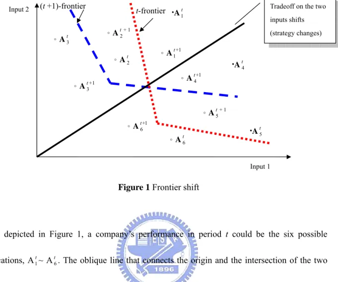
Figure 1 Frontier shift

As depicted in Figure 1, a company’s performance in period t could be the six possible

locations, At

1~ A

t

6. The oblique line that connects the origin and the intersection of the two frontiers is the tradeoff on the strategy changes. At

1, A

t

2, and A

t

3 locate on the upper part and inside the t-frontier, between the two frontiers, and outside the (t+1)-frontier respectively. The

distances of At

2 and A

t

3 to the t- and (t+1)-frontiers respectively are the measurement of super-efficiencies. Similarly, At

4, A

t

5, and A

t

6 locate on the lower part and inside the

(t+1)-frontier, between the two frontiers, and outside the t-frontier respectively. The distances

of A t

6 and A 5

t _{to the t- and (t+1)-frontiers respectively are the measurement of}

super-efficiencies. It is noticeable that the locations of the six points A +1 1 t _~A +1 6 t _{have similar} occasions. (t +1)-frontier ·A₁t t-frontier ·At₄ ·At₅ 。At₄+1 。A₁t+1 。At₂+1 。At₂ 。At₃ 。A₃t+1 。A₅t+1 。At₆+1 。At₆ Input 1

Input 2 Tradeoff on the two

inputs shifts (strategy changes)

express the efficiency measurement of each point by the ratio of distances; for instance, by drawing a line that connects the origin and point A +1

1

t _{. The line intersects with the t-frontier}

and (t+1)-frontier at points α1 and β1, respectively. The ratio of Dt(x_ot+1,yt_o+1) to

) , ( +1 +1 1 + t o t o t _{x y} D could be expressed as ₊₁ 1 1 At O α O and ₊₁ 1 1 At O β O , respectively. Thus, ) , ( ) , ( 1 + 1 + 1 + 1 + 1 + t o t o t t o t o t y x D y x D = 1 1 O O α

β . Similarly, drawing a line connects the origin and point A

t

1. The line intersects with the t-frontier and (t+1)-frontier at points γ1 and δ1, respectively. Tables 1 and 2

depict the models employed to measure the two distances. The signs of R1 and R2 in the last

columns are visible from Figure 1.

In Figure 1, a downward frontier shift (towards the origin) from period t to (t+1)

represents a positive shift. The converse situation (away from the origin) represents a negative shift. For a company, from period t to (t+1), the four possible frontier shifts are as follows in

(a)~(d). The 36 possible movements are depicted in Table 3.

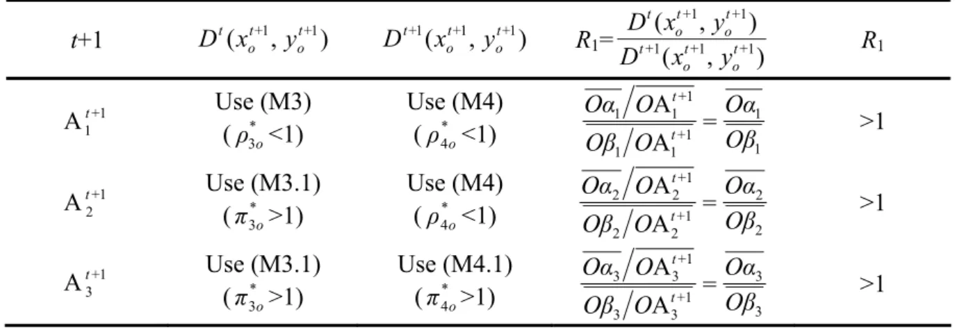
Table 1 The computation of ratio R1

t+1 ( +1, t+1) o t o t _{x y} D +1( +1, t+1) o t o t _{x y} D R1= ) , ( ) , ( 1 + 1 + 1 + 1 + 1 + t o t o t t o t o t y x D y x D R1 A +1 1 t Use (M3) ( * 3o ρ <1) Use (M4) ( * 4o ρ <1) 1 1 1 + 1 1 1 + 1 1 ₌ A A β O α O O β O O α O t t >1 A +1 2 t Use (M3.1) ( * 3o π >1) Use (M4) ( * 4o ρ <1) 2 2 1 + 2 2 1 + 2 2 ₌ A A β O α O O β O O α O t t >1 A +1 3 t Use (M3.1) (_{π >1)} * Use (M4.1) (_{π >1)} * ₊₁ 3 1 + 3 3 ₌ A A β O α O O β O O α O t t >1

A +1 4 t Use (M3) ( * 3o ρ <1) Use (M4) ( * 4o ρ <1) 4 4 1 + 4 4 1 + 4 4 = A A β O α O O β O O α O t t <1 A +1 5 t Use (M3) ( * 3o ρ <1) Use (M4.1) ( * 4o π >1) 5 5 1 + 5 5 1 + 5 5 ₌ A A β O α O O β O O α O t t <1 A +1 6 t Use (M3.1) ( * 3o π >1) Use (M4.1) ( * 4o π >1) 6 6 1 + 6 6 1 + 6 6 = A A β O α O O β O O α O t t <1

Table 2 The computation of ratio R2

t ( , t) o t o t _{x y} D +1( , t) o t o t _{x y} D R2= ) , ( ) , ( 1 + t o t o t t o t o t y x D y x D R2 At 1 Use (M1) ( * 1o ρ <1) Use (M2) ( * 2o ρ <1) 1 1 1 1 1 1 ₌ A A δ O γ O O δ O O γ O t t >1 At 2 Use (M1.1) ( * 1o π >1) Use (M2) ( * 2o ρ <1) 2 2 2 2 2 2 ₌ A A δ O γ O O δ O O γ O t t >1 At 3 Use (M1.1) ( * 1o π >1) Use (M2.1) ( * 2o π >1) ₃3 3 3 3 3 ₌ A A δ O γ O O δ O O γ O t t >1 At 4 Use (M1) ( * 1o ρ <1) Use (M2) ( * 2o ρ <1) 4 4 4 4 4 4 ₌ A A δ O γ O O δ O O γ O t t <1 At 5 Use (M1) ( * 1o ρ <1) Use (M2.1) ( * 2o π >1) 5 5 5 5 5 5 = A A δ O γ O O δ O O γ O t t <1 At 6 Use (M1.1) ( * 1o π >1) Use (M2.1) ( * 2o π >1) 6 6 6 6 6 6 ₌ A A δ O γ O O δ O O γ O t t <1

Table 3 The four possible frontier shifts for a company between two periods To period (t+1)

A₁t+1 A₂t+1 A₃t+1 A₄t+1 A₅t+1 A₆t+1 At₁

At₂ At₃

(a) R2>1 and R1>1 (d) R2>1 and R1<1

At₄ From period t

At

At₆

(a) If R2>1 and R1>1,

then the FSo must be larger then 1.0, indicating the DMUo has a positive shift and the

technology of DMUo progresses. As shown in Figure 1, the points of period t, A₁t, At₂, and At₃

in the upper part could be one of the points at period (t+1) in the upper part, A +1

1t , A2t+1, and A +1

3

t _.

(b) If R2<1 and R1<1,

then the FSo must be less then 1.0, indicating the DMUo has a negative shift and the

technology of DMUo declines. As shown in Figure 1, the points of period t, At₄, At₅, and At₆

in the lower part could be one of the points at period (t+1) in the lower part, A +1 4 t _{, A} +1 5 t _{, and} A +1 6 t _. (c) If R2<1 and R1>1,

then FSo may be larger or less then 1.0. But, certainly we can conclude DMU_o moves from a

negative shift facet towards a positive shift facet. Also, there is a change in the tradeoff between the two inputs. Furthermore, FSo <1 indicates that the change resulting from the

positive shift facet is less than that of the negative shift facet; and, on average, the technology of DMUo declines. In contrast, FSo >1 indicates that the change resulting from the positive

shift facet is lager than that of the negative shift facet; and, on average, the technology of

same. As shown in Figure 1, the points of period t, At

4, A

t

5, and A

t

6 in the lower part could be one of the points at period (t+1) in the upper part, A +1

1 t _{, A} +1 2 t _{, and A} +1 3 t _. (d) If R2>1 and R1<1,

then FSo may be greater or less then 1.0. But, we can certainly conclude DMUo moves from a

positive shift facet towards a negative shift facet. Also, there is a change in the tradeoff between the two inputs. Furthermore, FSo <1 indicates that the change resulting from the

positive shift facet is less than that of the negative shift facet; and, on average, the technology of DMUo declines. In contrast, FSo >1 indicates that the change resulting from the positive

shift facet is lager than that of the negative shift facet; and, on average, the technology of

DMUo progresses. FSo =1 indicates that on average the technology of DMUo remains the same.

As shown in Figure 1, the points of period t, At

1, A

t

2, and A

t

3 in the upper part could be one of the points at period (t+1) in the lower part, A +1

4 t _{, A} +1 5 t _{, and A} +1 6 t _. 3.1 Definition of TECo Note that Mt+1

o = TECo× FSo and TECo =Dt 1(xot 1,yot 1) Dt(xot,yot)

+ + + _{if (i) TEC} o >1, indicating +1( +1, t+1) o t o t _{x y} D > ( , t) o t o t _{x y}

D . This implies that DMUo in time (t+1) is closer to the

frontier in time t, (ii) TECo <1 implies DMUo in time (t+1) is further away from the frontier in

(t+1) than DMUo in time t to the frontier in t, and (iii) TECo=1 implies DMUo in time (t+1) is

4. An application

We employ the proposed approach to analyze the performance changes in semiconductor packaging and testing firms in Taiwan between the years 2000 and 2003. Among them, 15 companies chosen by Liu and Yang (2004) are further analyzed in this study. The calculations are based upon one input, Liability ratio, and four outputs: (i) Growth rate (%), (ii) Net profit after tax ($100 million NT dollars), (iii) Profitability ratio (%), and (iv) Output value by employee ($million/people).

4.1 Data collection and index description

In recent years, many semiconductor packaging and testing firms have been founded and their sales value has increased rapidly. This study uses the data published in the popular business magazine Common Wealth (2004) to analyze the relative performance of these firms between 2000 and 2003. The profile of the firms over these four years is listed in Table 4 and Table 5 that report the total profile of all firms in each year and the inputs/outputs of the 15 firms respectively.

Table 4 Profile of the firms, 2000-2003

2000 2001 2002 2003 Revenue ($100 million US dollars) 33.19 25.38 31.52 38.21 Total assets ($100 million US dollars) 76.13 74.12 74.20 82.00 Capital ($100 million US dollars) 27.17 32.23 32.55 34.62

Liability ($100 million US dollars) 14.08 13.55 14.33 15.39

Number of employees 34,106 31,055 34,149 42,228

The following table shows five indices in Common Wealth: (i) Y₁= Growth Rate (%), (ii) Y₂= Net profit after tax ($100 million NT dollars), (iii) Y₃= Profitability ratio (%), (iv) Y₄= Output value by employee ($million/people), and (v) X₁= Liability ratio (%). These indices have been commonly used in most of financial statements for analyzing a performance of companies or enterprises. The choice secures the reliability for the current approach in this thesis.

Table 5 Basic Data

Index DMU Firm Y1 Y2 Y3 Y4 X1 Year 2000 1 ASE 145.86 98.37 122.87 3.50 38.26 2 SIPIN 158.16 72.21 117.09 3.56 32.84 3 OSE 146.85 41.04 100.73 2.19 31.12 4 ChipMos 128.82 55.39 118.71 4.11 33.80 5 KYEC 239.66 51.78 128.17 1.41 43.37 6 ASE Chung Li 284.76 55.90 121.02 3.47 50.90 7 Sharp in Taiwan 157.53 58.19 135.43 3.31 28.55 8 Greatek 154.48 45.25 114.15 2.68 44.83 9 Lingsen 153.12 43.38 110.27 2.07 26.09 10 PowerTech 344.42 42.50 118.85 1.46 56.07 11 UTC 136.54 49.02 125.65 4.49 23.01 12 KingPak 200.28 38.75 98.05 22.27 53.41 13 Hi-Sincerity 100.75 40.25 101.68 12.37 38.89 14 Formosa 143.13 41.77 110.24 2.37 58.83 15 Sigurd 135.29 41.50 114.49 1.98 32.05 Year 2001 1 ASE 80.35 18.57 89.55 3.40 41.46 2 SIPIN 87.71 28.17 92.84 2.50 38.11 3 OSE 75.04 8.10 70.14 1.98 56.19 4 ChipMos 65.79 24.91 72.58 3.24 31.91

6 ASE Chung Li 64.80 40.57 101.16 2.66 38.12 7 Sharp in Taiwan 78.55 37.60 94.05 2.75 25.01 8 Greatek 89.43 42.48 107.48 2.74 41.80 9 Lingsen 71.17 41.25 105.34 1.87 20.73 10 PowerTech 234.47 41.73 105.56 3.57 43.30 11 UTC 38.25 31.10 33.83 2.43 24.64 12 KingPak 33.53 39.17 96.14 7.68 48.35 13 Hi-Sincerity 70.15 40.21 102.02 11.32 37.24 14 Formosa 59.51 41.22 111.86 1.76 58.27 15 Sigurd 82.70 40.08 100.93 1.91 26.29 Year 2002 1 ASE 125.00 41.29 100.50 4.20 42.50 2 SIPIN 134.90 44.25 101.91 2.79 43.28 3 OSE 119.56 7.00 74.16 2.65 64.18 4 ChipMos 118.57 27.92 81.49 3.21 44.48 5 KYEC 137.94 36.97 94.33 1.76 49.08 6 ASE Chung Li 105.22 43.66 107.09 2.29 30.66 7 Sharp in Taiwan 118.37 37.99 95.79 2.74 32.12 8 Greatek 134.67 46.34 114.19 3.36 36.48 9 Lingsen 125.40 36.33 87.51 2.13 25.67 10 PowerTech 90.74 41.87 106.63 2.80 34.86 11 UTC 159.26 36.73 84.73 3.17 22.31 12 KingPak 98.79 38.87 94.68 4.38 54.26 13 Hi-Sincerity 96.83 39.64 96.43 11.59 39.12 14 Formosa 162.59 40.92 105.50 2.51 55.16 15 Sigurd 143.22 42.38 120.12 2.31 43.77 Year 2003 1 ASE 122.85 67.43 108.71 3.11 41.08 2 SIPIN 122.80 68.39 110.37 2.99 45.06 3 OSE 105.91 5.64 74.60 2.72 66.88 4 ChipMos 129.77 48.61 110.17 3.36 39.43 5 KYEC 126.91 47.73 111.39 2.38 33.89 6 ASE Chung Li 116.65 41.83 103.04 2.08 34.23 7 Sharp in Taiwan 140.26 51.91 117.79 2.68 34.58 8 Greatek 116.10 49.27 117.88 3.42 35.63 9 Lingsen 133.22 43.69 109.43 2.43 30.28 10 PowerTech 155.44 50.40 123.72 3.21 45.67 11 UTC 107.53 39.92 99.63 2.93 19.95 12 KingPak 59.82 40.94 107.40 2.87 44.82 13 Hi-Sincerity 101.98 39.35 93.68 11.05 40.29 14 Formosa 122.77 41.91 109.30 2.90 54.62 15 Sigurd 149.37 44.18 123.66 2.47 34.16

Table 6 DEA technical efficiency from 2000 to 2003 Firms Dt(xot,yot) 2000 2001 2002 2003 ASE 1.038 0.414 0.558 0.584 SIPIN 0.762 0.504 0.518 0.530 OSE 0.525 0.174 0.156 0.114 ChipMos 0.665 0.549 0.428 0.591 KYEC 0.349 0.250 0.342 0.618 ASE Chung Li 0.490 0.533 0.642 0.548 Sharp in Taiwan 0.807 0.864 0.638 0.664 Greatek 0.423 0.532 0.668 0.651 Lingsen 0.659 1.163 0.731 0.687 PowerTech 1.009 1.101 0.562 0.546 UTC 1.185 0.479 1.246 1.345 KingPak 1.093 0.418 0.394 0.377 Hi-Sincerity 0.734 1.161 1.150 1.131 Formosa 0.288 0.269 0.401 0.390 Sigurd 0.485 0.756 0.485 0.646 Industry average 0.701 0.611 0.595 0.628

Table 7 Technical efficiency change

Firms TEC 2000 vs. 2001 2001 vs. 2002 2002 vs. 2003 ASE 0.399 1.349 1.046 SIPIN 0.662 1.028 1.022 OSE 0.331 0.897 0.728 ChipMos 0.825 0.781 1.380 KYEC 0.715 1.370 1.807 ASE Chung Li 1.088 1.206 0.853 Sharp in Taiwan 1.071 0.739 1.041 Greatek 1.256 1.257 0.975 Lingsen 1.764 0.629 0.939 PowerTech 1.091 0.510 0.972 UTC 0.404 2.601 1.080 KingPak 0.383 0.942 0.957 Hi-Sincerity 1.581 0.990 0.984 Formosa 0.934 1.489 0.972 Sigurd 1.557 0.642 1.331

Tables 6 and 7 report the DEA technical efficiency and the associated technical efficiency changes from 2000 to 2003. From Table 6, Hi-Sincerity is the only one improving its performance year after year. Figure 2 shows its technical efficiency in 2000 to be less than 1.0 but larger than 1.0 afterwards. However, the technical change for Hi-Sincerity shown in Table 7 is larger than 1.0 only between 2000 and 2001, but less than 1.0 in the remaining years, indicating an exact definition of technical efficiency progress still needs to be investigated; all technical changes larger than or equal to 1.0 would be perfect, generally. Note that, in Table 7, only KingPak and OSE do not show technical efficiency progress from 2000 to 2003; on the other hand, we can conclude that other firms show improvement and decline in technical efficiency change. For the industry average, technical efficiency declines 6.3% from 2000 to 2001, improves 9.5% from 2001 to 2002, and improves 7.3% from 2002 to 2003.

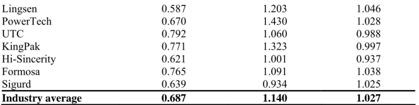
Table 8 Frontier shift

Firms FS 2000 vs. 2001 2001 vs. 2002 2002 vs. 2003 ASE 0.853 1.133 1.034 SIPIN 0.709 1.139 1.034 OSE 0.664 0.998 1.137 ChipMos 0.694 1.142 1.052 KYEC 0.521 1.041 0.996 ASE Chung Li 0.590 1.216 1.021 Sharp in Taiwan 0.708 1.214 1.041 Greatek 0.720 1.177 1.031

Lingsen 0.587 1.203 1.046 PowerTech 0.670 1.430 1.028 UTC 0.792 1.060 0.988 KingPak 0.771 1.323 0.997 Hi-Sincerity 0.621 1.001 0.937 Formosa 0.765 1.091 1.038 Sigurd 0.639 0.934 1.025 Industry average 0.687 1.140 1.027

Table 8 reports the Malmquist frontier shift component. It can be seen that on average, the industry technology frontier declines 31.3% from 2000 to 2001, improves 23.8% from 2001 to 2002, and improves 2.3% from 2002 to 2003.

As indicated by FSo in Table 8, we can see all firms show negative shift in technology

frontier from 2000 to 2001. From 2001 to 2002, only Sigurd and OSE show a negative shift in technology frontier, indicating the period has changed drastically compared with the previous period. Regarding the periods 2002 to 2003, although most of the firms declines in frontier shift compared with 2001 to 2002, they still hold a positive frontier shift (FSo>1). Over this

period, only four firms, KYEC, Hi-Sincerity, UTC, and KingPak show a negative frontier shift; the other 11 firms still show a positive shift.

In the previous section, FSo is known as a product of two ratios,

) , ( ) , ( +1 +1 +1 +1 t+1 o t o t t o t o t _{x y D x y} D and ( , ) 1( , t) o t o t t o t o t _{x y D x y}

D + . Moreover, the value of each ratio represents a different implication; thus, we still need to discuss the two components of FSo.

Note that R1=Dt(xot+1,yot+1) Dt+1(xot+1,yot+1), R2=Dt(xot,yot) Dt 1(xot,yot)

+

in the following table (Chen and Ali, 2004).

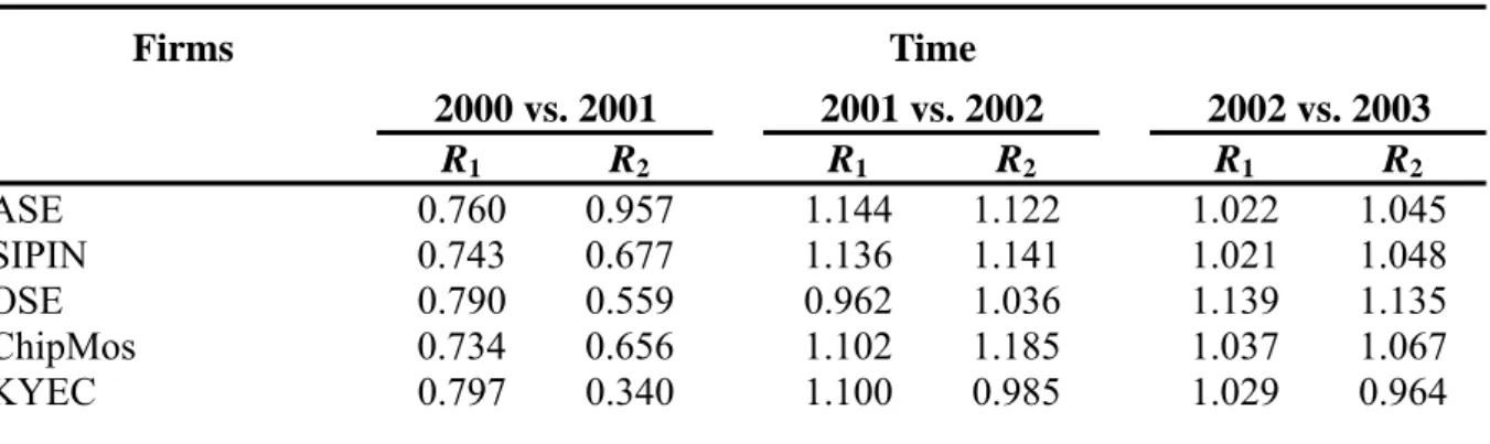
Table 9 reports the component shifts in technical frontier. We can see that no firms show a cross-frontier shift from 2000 to 2001, corresponding with the fact that no one shows a positive frontier shift in Table 8. From 2001 to 2002, take OSE, UTC, and Hi-Sincerity as examples, their R1 <1 and R2 >1 indicate they move from a positive shift facet towards a

negative shift facet. In terms of management, this situation should be avoided. However, other firms all show the pure positive shift (R1>1, R2 >1), indicating they stand for consistent

operation strategies. From 2002 to 2003, we can find out the cause of four firms’ frontier shift less than 1.0 (Table 8). Among these four firms, only the cause of KYEC’s frontier shift less than 1.0 is R1>1 can not overcome the damage from R2<1; the cause of the others’ is their

R1<1 covers the positive effect from R2>1. Except these four firms, all show the pure positive

frontier shift. For the industry average, it is worth noting there is a negative frontier shift from 2000 to 2001, but that it moves to a desirable shift from 2001 to 2003. Commonly, only a minority of the firms show that moving from a good shift facet to a bad shift facet (R1<1, R2

>1).

Table 9 Individual shift

Firms Time 2000 vs. 2001 2001 vs. 2002 2002 vs. 2003 R1 R2 R1 R2 R1 R2 ASE 0.760 0.957 1.144 1.122 1.022 1.045 SIPIN 0.743 0.677 1.136 1.141 1.021 1.048 OSE 0.790 0.559 0.962 1.036 1.139 1.135 ChipMos 0.734 0.656 1.102 1.185 1.037 1.067

ASE Chung Li 0.726 0.480 1.205 1.227 1.018 1.023 Sharp in Taiwan 0.709 0.708 1.203 1.225 1.036 1.045 Greatek 0.755 0.687 1.213 1.143 1.022 1.040 Lingsen 0.566 0.609 1.392 1.039 1.041 1.052 PowerTech 0.459 0.979 1.177 1.736 1.045 1.010 UTC 0.729 0.861 0.928 1.210 0.834 1.169 KingPak 0.631 0.942 1.168 1.499 0.968 1.028 Hi-Sincerity 0.551 0.700 0.892 1.124 0.783 1.122 Formosa 0.765 0.765 1.106 1.077 1.038 1.039 Sigurd 0.696 0.587 1.158 0.754 1.041 1.009 Industry average 0.694 0.700 1.126 1.167 1.005 1.053

Table 10 Malmquist productivity

Firms Mt_o+1 2000 vs.2001 2001 vs.2002 2002 vs.2003 ASE 0.34 1.528 1.081 SIPIN 0.469 1.170 1.057 OSE 0.220 0.895 0.828 ChipMos 0.573 0.892 1.451 KYEC 0.373 1.426 1.799 ASE Chung Li 0.642 1.467 0.871 Sharp in Taiwan 0.759 0.897 1.083 Greatek 0.904 1.480 1.005 Lingsen 1.035 0.756 0.983 PowerTech 0.732 0.729 0.999 UTC 0.320 2.757 1.067 KingPak 0.295 1.247 0.955 Hi-Sincerity 0.982 0.992 0.923 Formosa 0.715 1.625 1.009 Sigurd 0.996 0.600 1.364 Industry average 0.624 1.231 1.098

Table 10 reports the Malmquist productivity index Mt+1

o . It can be seen, on industry

average, there is about a 37.6% productivity loss from 2000 to 2001, while from 2001 to 2002 there is about a 23.1% productivity gain and from 2002 to 2003 there is about a 9.8% productivity gain.

is, Mt+1

o = TECo×FSo. In order to analyze the performances of these firms more precisely, the

information in Tables 7 and 8 is not only helpful, but essential. Fortunately, Mt+1

o is consistent

with TECo and FSo here. However, if we see that the Malmquist productivity index is larger

than 1.0 on average in a certain case, this is maybe a combined effect of an average improvement in technology frontier and an average declining technical efficiency. Such a situation does not appear in this case, but it would be absolutely necessary for management to make a detailed investigation to find the real cause of productivity gains or losses.

Therefore, for the conclusion regarding productivity change of each firm, we must refer to FSo and TECo. In addition, Table 11 is derived comprehensively as follows.

Next, let us examine the detailed Malmquist change information. Here, we denote R1

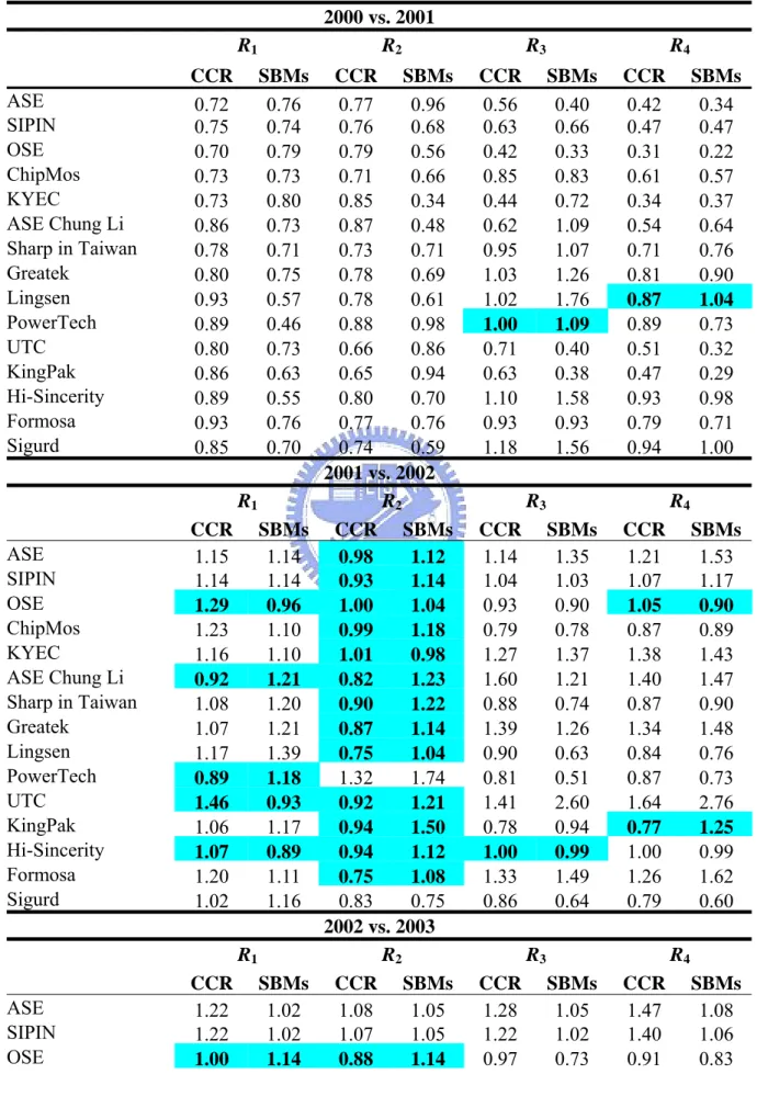
(first component of FS) = ( +1, +1) +1( +1, t+1) o t o t t o t o t _{x y D x y} D , R2 (second component of FS) = ( , ) 1( , t) o t o t t o t o t _{x y D x y} D + , R3 (TEC) = Dt+1(x_ot+1,y_ot+1) Dt(x_ot,y_ot) , R4 (M t_o+1 ) = 2 1 1 1 1 1 1 1 ) , ( ) , ( ) , ( ) , ( ⎥ ⎥ ⎦ ⎤ ⎢ ⎢ ⎣ ⎡ + + + + + + t o t o t t o t o t t o t o t t o t o t y x D y x D y x D y x D .

Table 11 reports the component information associated with productivity change. Contents include results of CCR models and SBM/Super-SBM models. In the previous instruction, the value of each ratio presents different management implication when >1, =1, <1. Thus, differences are highlighted for readers to note them easily. “SBMs” denotes the results of SBM/Super-SBM models.

Table 11 Detailed Malmquist productivity change information 2000 vs. 2001 R1 R2 R3 R4 CCR SBMs CCR SBMs CCR SBMs CCR SBMs ASE _{0.72 0.76 0.77 0.96 0.56 0.40 0.42 0.34} SIPIN 0.75 0.74 0.76 0.68 0.63 0.66 0.47 0.47 OSE 0.70 0.79 0.79 0.56 0.42 0.33 0.31 0.22 ChipMos 0.73 0.73 0.71 0.66 0.85 0.83 0.61 0.57 KYEC 0.73 0.80 0.85 0.34 0.44 0.72 0.34 0.37 ASE Chung Li 0.86 0.73 0.87 0.48 0.62 1.09 0.54 0.64 Sharp in Taiwan 0.78 0.71 0.73 0.71 0.95 1.07 0.71 0.76 Greatek 0.80 0.75 0.78 0.69 1.03 1.26 0.81 0.90 Lingsen 0.93 0.57 0.78 0.61 1.02 1.76 0.87 1.04 PowerTech 0.89 0.46 0.88 0.98 1.00 1.09 0.89 0.73 UTC 0.80 0.73 0.66 0.86 0.71 0.40 0.51 0.32 KingPak 0.86 0.63 0.65 0.94 0.63 0.38 0.47 0.29 Hi-Sincerity 0.89 0.55 0.80 0.70 1.10 1.58 0.93 0.98 Formosa 0.93 0.76 0.77 0.76 0.93 0.93 0.79 0.71 Sigurd 0.85 0.70 0.74 0.59 1.18 1.56 0.94 1.00 2001 vs. 2002 R1 R2 R3 R4 CCR SBMs CCR SBMs CCR SBMs CCR SBMs ASE 1.15 1.14 0.98 1.12 1.14 1.35 1.21 1.53 SIPIN 1.14 1.14 0.93 1.14 1.04 1.03 1.07 1.17 OSE 1.29 0.96 1.00 1.04 0.93 0.90 1.05 0.90 ChipMos 1.23 1.10 0.99 1.18 0.79 0.78 0.87 0.89 KYEC 1.16 1.10 1.01 0.98 1.27 1.37 1.38 1.43 ASE Chung Li 0.92 1.21 0.82 1.23 1.60 1.21 1.40 1.47 Sharp in Taiwan 1.08 1.20 0.90 1.22 0.88 0.74 0.87 0.90 Greatek 1.07 1.21 0.87 1.14 1.39 1.26 1.34 1.48 Lingsen 1.17 1.39 0.75 1.04 0.90 0.63 0.84 0.76 PowerTech 0.89 1.18 1.32 1.74 0.81 0.51 0.87 0.73 UTC 1.46 0.93 0.92 1.21 1.41 2.60 1.64 2.76 KingPak 1.06 1.17 0.94 1.50 0.78 0.94 0.77 1.25 Hi-Sincerity 1.07 0.89 0.94 1.12 1.00 0.99 1.00 0.99 Formosa 1.20 1.11 0.75 1.08 1.33 1.49 1.26 1.62 Sigurd 1.02 1.16 0.83 0.75 0.86 0.64 0.79 0.60 2002 vs. 2003 R1 R2 R3 R4 CCR SBMs CCR SBMs CCR SBMs CCR SBMs ASE 1.22 1.02 1.08 1.05 1.28 1.05 1.47 1.08 SIPIN 1.22 1.02 1.07 1.05 1.22 1.02 1.40 1.06

ChipMos 1.22 1.04 0.99 1.07 1.26 1.38 1.38 1.45 KYEC 1.23 1.03 0.97 0.96 1.39 1.81 1.52 1.80 ASE Chung Li 1.25 1.02 1.29 1.02 0.69 0.85 0.88 0.87 Sharp in Taiwan 1.21 1.04 1.15 1.05 0.96 1.04 1.13 1.08 Greatek 1.26 1.02 1.20 1.04 0.84 0.97 1.03 1.00 Lingsen 1.17 1.04 0.99 1.05 0.91 0.94 0.98 0.98 PowerTech 1.13 1.05 1.31 1.01 0.78 0.97 0.96 1.00 UTC 1.31 0.83 0.76 1.17 1.00 1.08 1.00 1.07 KingPak 1.31 0.97 1.13 1.03 0.99 0.96 1.20 0.96 Hi-Sincerity 0.95 0.78 0.93 1.12 1.00 0.98 0.94 0.92 Formosa 1.26 1.04 0.92 1.04 0.83 0.97 0.89 1.01 Sigurd 1.17 1.04 1.19 1.01 1.12 1.33 1.33 1.36

“ , the blue highlighted or the boldface”: indicates the different between radial- and slacks-based models.

In Table 11, among the 180 comparisons of two measurement methods, 39 (21.7%) are in different signs, a large percentage of total. This proves the current SBM-based approach indeed revises the weak points of the radial-based measure, leading to an appropriate result. It is obvious that applying the current approach leads to a different managerial interpretation. Theoretically, SBM/Super-SBM models have a truly specific interpretation in these 15 firms. One of the major reasons for the difference is that previous study did not measure the super-efficiency of DMUo in a single period t or (t+1). The more explicit explanation is in

Section 5. The following table shows the extracted results of SBM/Super-SBM from Table 11. (a)~(d) denote the four definitions cases of R1 and R2 in Section 3; D denotes “Decline”; P

Table 12 Detailed Malmquist productivity change information of SBM/Super-SBM

2000 vs. 2001 2001 vs. 2002 2002 vs. 2003

R1, R2 R3 R4 R1, R2 R3 R4 R1, R2 R3 R4

ASE (b) D D (a) P P (a) P P

SIPIN (b) D D (a) P P (a) P P

OSE (b) D D (d) D D (a) D D

ChipMos (b) D D (a) D D (a) P P

KYEC (b) D D (c) P P (c) P P

ASE Chung Li (b) P D (a) P P (a) D D

Sharp in Taiwan (b) P D (a) D D (a) P P

Greatek (b) P D (a) P P (a) D P

Lingsen (b) P P (a) D D (a) D D

PowerTech (b) P D (a) D D (a) D D

UTC (b) D D (d) P P (d) P P

KingPak (b) D D (a) D P (d) D D

Hi-Sincerity (b) P D (d) D D (d) D D

Formosa (b) D D (a) P P (a) D P

Sigurd (b) P D (c) D D (a) P P

We will first expand on the managerial purpose concerning the results of SBM and Super-SBM measures in Table 12. We advice that referring to the definitions of (a) ~(d) in Section 3 and signs D and P in Table 12 could be more understandable for the following analysis. By analyzing some meaningful cases, we will determine the essential factor of each productivity result. First, the Malmquist productivity of PowerTech are both decline in two periods – from 2000 to 2001 and from 2001 to 2002 – yet the contents of R1, R2 and R3 in

each period are contrary. From 2000 to 2001, the components of FSo display a pure negative

technical efficiency progress, while the components of FSo reveal purely positive.

Secondly, PowerTech shows a productivity loss from 2002 to 2003 due to improvement in FSo where R1 and R2 are both >1 (case(a)), and the only decline in technical efficiency,

representing the positive frontier shift cannot overtake the harm from technical efficiency decline. In terms of chasing a good performance, management strategy should focus on this issue.

UTC shows productivity gain with an improvement in technical efficiency from 2001 to

2002. Actually, the firm is moving to a negative shift facet because the R1<1 and R2 >1. The

implication of these two ratios has been discussed previously. Therefore, UTC demonstrates an unfavorable strategy in this period.

Hi-Sincerity from 2001 to 2002 shows the least favorable strategy for change under the

scenario R1 and R2 performing inconsistently, case (c) and (d). Since its R4 progresses, R3

declines, the performance of R1, R2 corresponds to case (d), we can conclude that it also

suffers productivity loss, technical efficiency change decline, and has moved from a positive shift facet towards a negative shift facet. This situation must be discussed because every company or industry may encounter such potential danger, and it is easily ignored.

Among the current set of performance assessments of semiconductor packaging and testing firms in Taiwan, KYEC is the polar opposite of Hi-Sincerity. It is significant to know that the most favorable strategy change occurs when R4>1, R3>1, the performance of R1, R2

correspond to case (c) under the scenario that R1 and R2 perform inconsistently. In other words,

the conditions demonstrate that besides the particular company showing productivity gain and progress in technical efficiency, its strategy moves from a negative shift facet towards a positive shift facet.

The last two simple cases are (i) R4 >1, R3>1, and R1>1, R2 >1(case(a)), which indicates

the best result of all, and (ii) R4 <1, R3 <1, and R1<1, R2<1 (case(b)), which indicates the

worst result of all. The above discussion shows that by further analyzing the Malmquist components, more insights into productivity changes can be obtained.

5. Comparisons of CCR and SBM measures

We compare our results and the results obtained by Chen and Ali (2004) employing the CCR model. As noted earlier in this thesis, *

o

θ , *

o

ρ , and *

o

π are the optimal efficiency scores of CCR, SBM, and Super-SBM models respectively. When measuring the distances

) , ( t o t o t _{x y} D and +1( +1, t+1) o t o t _{x y}

D , if the object company is inefficient, the CCR score *

o

θ is greater or equal to the SBM score. If the object company is efficient, we further measure its distance to the frontier constructed by the other companies; the Super-SBM efficiency scores are greater than 1.0 and greater than the CCR scores, 1.0. In the other case, we measure the distances across two periods of +1( , t)

o t o t _{x y} D and )( +1, t+1 o t o t _{x y}

D ; if the object company is inefficient, the CCR score *

o

θ is greater or equal to the SBM score. If the object company is efficient, we further measure its distance to the frontier constructed by all the companies in other periods; the Super-SBM efficiency scores are greater than 1.0 and greater than the CCR scores, 1.0.

Chen and Ali (2004) do not measure the Super-CCR efficiency score (Andersen & Petersen, 1993) of DMUo in a single period t or (t+1); therefore, πo*≧1, θo*≦1 and verified

that *

o

π ≧θ_o*. As a result, the changes in optimal efficiency score for the three models might

affect the ratios R1, R2, R3, and R4.

Take R1 for example, measuring the two distance functions of R1

model could be inefficient or efficient. Their values are depicted in Table 13. The ratio R1

could be obtained by the three possible combinations as shown in Table 14, where I and E denote inefficient and efficient, respectively. Given the ratio R1 is less than 1.0 for the

SBM/Super-SBM models (R1, SBMs), the ratio R1 for the CCR model (R1, CCR) could be inferred.

The first and second combinations have different outcomes in two models. One could perform similar analysis for the ratios R2, R3, and R4 under the two models. The current thesis provides

measurement different from the CCR measure proposed by Chen and Ali (2004).

Table 13 Values of Dt(xt_o+1,y_ot+1) and Dt+1(x_ot+1,y_ot+1)

SBM/Super-SBM CCR Inefficient Efficient Inefficient Efficient ) , ( +1 t+1 o t o t _{x y} D ≦1 ≧1 ≦1 ≧1 ) , ( +1 +1 1 + t o t o t _{x y} D ≦1 ≧1 ≦1 1

Tabe 14 Values of [Dt(x_ot+1,y_ot+1) / Dt+1(x_ot+1,y_ot+1)] when R_{1,SBM/Super-SBM} ≤ 1

No. Combination R1,SBMs≤ 1 R1,CCR

1 I _I ≦1 ≦1

or 1≧

2 E _E ≦1 ≧1

6. Conclusions

We benefited from use of the DEA Malmquist productivity approach employed by Chen and Ali (2004) to discover that in-depth information could be obtained by analyzing each individual component of the Malmquist productivity index. Further, the result is more precise using the SBM/Super-SBM measures. According to the comparison with CCR, there are numbers of differences at the end. Such analyses not only help revise the weak points in the CCR model but also provide a more in-depth management implication. It is very critical to capturing a firm’s performance through an analysis of the components of the Malmquist productivity index to reveal the managerial implications of each component and limit misleading information. As a result, a firm will be aware of what kind of weaknesses they should watch out for and remedy. Furthermore, in terms of industrial management, this method allows judgments to be made concerning whether or not the strategic shift is favorable and promising.

Appendix

The relative efficiency of DMUo for (a, b) = (t, t+1).

* 3o ρ = ( +1, t+1) o t o t _{x y} D =Min k − m 1

∑

∑

∑

∑

The relative super efficiency of DMUo for (a, b) = (t, t+1).

∑

∑

∑

∑