利用熵選取門檻之自動彩色邊緣偵測

國 立 交 通 大 學

電 機 與 控 制 工 程 研 究 所

碩 士 論 文

利用熵選取門檻之自動彩色邊緣偵測

Automatic Color Edge Detection by Entropic Thresholding

研 究 生 ： 江宇洋

指 導 教 授： 張 志 永

利用熵選取門檻之自動彩色邊緣偵測

Automatic Color Edge Detection by Entropic Thresholding

學 生 : 江宇洋 Student : Yu-Yang Jiang

指導教授 : 張志永 Advisor : Jyh-Yeong Chang

國立交通大學

電機與控制工程學系

碩士論文

A Thesis

Submitted to Department of Electrical and Control Engineering

College of Electrical Engineering and Computer Science

National Chiao Tung University

in Partial Fulfillment of the Requirements

for the Degree of Master in

Electrical and Control Engineering

June 2009

Hsinchu, Taiwan, Republic of China

利用熵選取門檻之自動彩色邊緣偵測

學生: 江宇洋 指導教授: 張志永博士

國立交通大學電機與控制工程研究所

摘要

由於邊緣偵測被廣泛應用在許多不同的影像處理上，例如: 影像分割、物體 辨識追蹤、立體分析等；這些影像處理任務的效能受到邊緣偵測結果好壞的巨大 影響，所以邊緣偵測是個重要且不可忽視的基礎影像處理技術。為了得到更真實 的邊緣，彩色邊緣偵測已經受到越來越多的重視。過去影像處理著重黑白影像邊 緣偵測，不過灰階影像偵測邊緣時，往往不能偵測出具有相近灰階值但不同色彩 的邊緣，同時也因為人類的視覺能區分出數千個不同的顏色卻只能區分出大約二 十種的灰階，所以灰階影像失去許多彩色影像的邊緣資訊;近年來有越來越多關 於彩色邊緣偵測的研究，不過這些彩色邊緣的研究的結果也只達到一定程度的效 果，所以我們希望能夠提供比較有效的彩色邊緣偵測的方法。 本論文，我們提出基於向量階層統計與主要成分分析的彩色邊緣偵測技術， 並且利用熵達到自動選取門檻的自動彩色邊緣偵測。利用我們提出的自動彩色邊 緣偵測，不僅可以偵測到當相鄰物體具有相近的灰階值但不同色彩的邊緣，且門 檻是依據影像內容所自動最佳調整，而不需要手動選取，增加使用者的方便性與 信賴度。

Automatic Color Edge Detection by Entropic

Thresholding

STUDENT:Yu-Yang Jiang ADVISOR: Dr. Jyh-Yeong Chang

Institute of Electrical and Control Engineering National Chiao-Tung University

ABSTRACT

Edge detection is an important process in low level image processing because of its wide use in various tasks, including segmentation, object recognition, tracking, stereo analysis, image coding and many others. The performance of various subsequent image or video processing tasks is therefore greatly affected by the goodness of edge detection. To obtain the genuine edges, there has been an increased interest in color edge detection. Humans can differentiate thousands of colors compared to about two dozen shades of gray; hence, grayscale images do not carry all the edge information that human visual system (HVS) can detect.

In this thesis, we propose automatic color edge detection techniques based on vector order statistics and principal component analysis by entropic thresholding. Both methods employed improved entropic thresholding to determine the edge threshold. Our color edge detection techniques can detect edges when neighboring objects have different hues but with similar intensities, which cannot be detected by known grayscale or color edge detectors. Furthermore, by using entropic thresholding we can automatically determine an optimal threshold which is adaptive to different image contents without manual intervention. Edge detection by our proposed scheme is very user friendly and confident.

ACKNOWLEDGEMENTS

I would like to express my sincere gratitude to my advisor, Dr. Jyh-Yeong Chang for valuable suggestions, guidance, support and inspiration he provided. Without his advice, it is impossible to complete this research. Thanks are also given to all of my lab members for their suggestion and discussion.

Finally, I would like to express my deepest gratitude to my family for their concern, supports and encouragements.

Contents

摘要 ...………... i

ABSTRACT ……….…... ii

ACKNOWLEDGEMENTS ………. iii

Contents ………...……iv

List of Figures ……….. vii

List of Tables ………. xi

Chapter 1 Introduction ………1

1.1 Motivation ………1

1.2 Color Edge Detection ………2

1.3 Automatic Thresholding Technique ………3

1.4 Thesis Outline ………4

Chapter 2 Introduction to Vector Order Statistics and Princicipal Component Analysis ………5

2.1 Vector Order Statistics ………5

2.1.1 Vector Order Statistics Review ………5

2.2 Principal Component Analysis ………8

2.2.1 Principal Component Analysis Review ………8

2.2.2 Characteristics of Principal Components ………9

2.2.3 Principal Component Vectors Computation ………11

Chapter 3 Color Edge Detection and Entropic Thresholding ………13

3.1 Vector Order Statistics based Color Edge Detection ………13

3.1.1 Confined Window Case ………13

3.1.2 Local Window Case ………16

3.2 PCA Based Edge Detection ………19

3.2.1 YC C Color Space ………19 _{b r} 3.2.2 Eigencolor Image Construction ………20

3.2.3 Edge Response Calculation ………21

3.3 Entropic Thresholding ………23

3.3.1 Entropic Thresholding for Vector Order Statistics based Edge Detection ………23

Chapter 4 Experimental Results ...27

4.1 Vector Order Statistics based Edge Detection ………27

4.2 PCA based Edge Detection ………40

4.3 Comparing the Experimental Results ………47

Chapter 5 Conclusion and Future Work ………62

List of Figures

Fig. 3.1. A simple edge example. (a) single edge image, (b) R-component values in

edge area, (c) the aggregate distances, and (d) sorted pixels vectors corresponding to

the same ordering of the aggregate distances, (e) the local sum of distances, and (f)

Sorted pixels vectors corresponding to the same ordering of the local sum of

distances ………. 18

Fig. 3.2. Sobel operator. (a) horizontal derivative approximation (b) vertical

derivative approximation ………..22 , i h g i v g

Fig. 4.1. Edge detection results of a color image with the same intensity. (a) original image, (b) edge detection by VMD, (c) edge detection by VDD, (d) edge detection by MD ………. 28 Fig. 4.2. The corresponding histograms of local optimal threshold to Fig. 4.1(a).

(a) histogram of

l

T∗

l

T∗ using VMD, (b) histogram of T_l∗ using VDD, (c) histogram of using MD.………29

l

T∗

Fig. 4.3. Edge detection results of a color image with different intensities. (a)

original image, (b) edge detection by VMD, (c) edge detection by VDD, (d) edge

detection by MD. ……… 31

Fig. 4.4. The corresponding histograms of local optimal threshold to Fig. 4.3(a).

(a) histogram of

l

T∗

l

l

T∗ using MD. ……… 32 Fig. 4.5. Edge detection results of a color image with different intensities. (a)

original image, (b) edge detection by VMD, (c) edge detection by VDD, (d) edge

detection by MD. ……… 33

Fig. 4.6. The corresponding histograms of local optimal threshold to Fig. 4.5(a).

(a) histogram of

l

T∗

l

T∗ using VMD, (b) histogram of T_l∗ using VDD, (c) histogram of using MD. ……… 34

l

T∗

Fig. 4.7. Edge detection results of a color image with diagonal edges. (a) original

image, (b) edge detection by VMD, (c) edge detection by VDD, (d) edge detection by

MD. ……… 36

Fig. 4.8. The corresponding histograms of local optimal threshold to Fig. 4.7(a).

(a) histogram of

l

T∗

l

T∗ using VMD, (b) histogram of T_l∗ using VDD, (c) histogram of using MD. ……… 37

l

T∗

Fig. 4.9. Edge detection results of a real world image. (a) original image, (b) edge

detection by VMD, (c) edge detection by VDD, (d) edge detection by MD.….…… 38

Fig. 4.10. Edge detection results of a human face image. (a) original image, (b) edge

detection by VMD, (c) edge detection by VDD, (d) edge detection by MD.………. 39

Fig. 4.11. Edge detection result of a color image with the same intensity. (a) original

Fig. 4.12. Edge detection result of a color image with the different intensities. (a)

original image, (b) the eigencolor image in RGB color space, (c) the edge detection

result.………... 42

Fig. 4.13. Edge detection result of a color image with diagonal edges. (a) original

image, (b) the eigencolor image in RGB color space, (c) the edge detection result... 43

Fig. 4.14. Fig. 4.14. The PDF and CDF of T_g∗ of the color image with diagonal edges. (a) PDF of Y, (b) CDF of Y (CDF of T_g∗=0.499), (c) PDF of C , (d) CDF of _b

b

C (CDF of T_g∗=0.504), (e) PDF of C_r, (f) CDF of C_r (CDF of T_g∗=0.501)…. 44 Fig. 4.15. Edge detection result of a real world image. (a) original image, (b) the

eigencolor image in RGB color space, (c) the edge detection result.…………..…... 45

Fig. 4.16. Edge detection result of a human face image. (a) original image, (b) the

eigencolor image in RGB color space, (c) the edge detection result.………. 46

Fig. 4.17. Edge detection result of a color image with the same intensity. (a) original

image, (b) VMD, (c) VDD, (d) MD, (e) eigencolor, (f) color Canny, (g) MVD, (h)

directional operator, (i) Dikbas et al. [18], (j) automatic isotropic color edge

detector.………...…. 50−51 Fig. 4.18. Edge detection result of a color image with the different intensities. (a)

original image, (b) VMD, (c) VDD, (d) MD, (e) eigencolor, (f) color Canny, (g) MVD,

detector.………..………...……... 52−53 Fig. 4.19. Edge detection result of a synthetic color image. (a) original image, (b)

VMD, (c) VDD, (d) MD, (e) eigencolor, (f) color Canny, (g) MVD, (h) directional

operator, (i) Dikbas et al. [18], (j) automatic isotropic color edge detector.….... 54 55 −

−

−

Fig. 4.20. Edge detection result of a real world image. (a) original image, (b) VMD, (c)

VDD, (d) MD, (e) eigencolor, (f) color Canny, (g) MVD, (h) directional operator, (i)

Dikbas et al. [18], (j) automatic isotropic color edge detector. .…………..…… 56 57

Fig. 4.21. Edge detection result of a real world image. (a) original image, (b) VMD, (c)

VDD, (d) MD, (e) eigencolor, (f) color Canny, (g) MVD, (h) directional operator, (i)

List of Tables

TABLE I. EVALUATION RESULT OF FOM, TPR, TNR, ACC AND NACC OF FIG.

4.17...60

TABLE II. EVALUATION RESULT OF FOM, TPR, TNR, ACC AND NACC OF FIG.

4.18...60

TABLE III. EVALUATION RESULT OF FOM, TPR, TNR, ACC AND NACC OF FIG. 4.19...…61

Chapter 1 Introduction

1.1 Motivation

Edge detection is an important process in low level image processing because of its wide use in several tasks such as segmentation, object recognition, tracking, stereo analysis, and image coding. The performance of these tasks is therefore tremendously affected by the goodness of edge detection. Conventionally, edge detectors use luminance component and locate changes in the intensity function. Pursuit of good edge detection algorithm led to such grayscale edge detectors as Canny, Cumani, and Compass [1]–[3]. Edges will not be detected in grayscale images when neighboring objects have different hues but equal intensities since the color cue is lost during grayscale conversion. Such objects cannot be distinguished in grayscale images. They are treated like one big object in the scene. This is not significant if the obstacle avoidance is the task of the vision system. Opposed to this, the capability of distinguishing between one big object and two (or several) objects may become crucial for the task of object grasping or even in 2-D image segmentation. Additionally, edge detection is sometimes difficult in low contrast images but rather sufficient results can be obtained in color images.

To obtain more meaningful edges, there has been an increased interest in color edge detection. Humans can differentiate thousands of colors compared to about two dozen shades of gray; hence, grayscale images do not carry all the edge information that human visual system (HVS) can detect. In [4], it is stated that luminance component makes up 90% of all edge points in a color image but the remaining 10% can be crucial for subsequent techniques that rely on edges in an image; in some cases the additional information provided by color is of utmost importance.

Multi-dimensional nature of color makes it more challenging to detect edges in color images, and often increases the computational complexity threefold compared to gray scale edge detection. Hence, color edge detection algorithms accept from the beginning that all of the efforts are to find the remaining 10% of the edges. Importance of color edge detection also becomes more apparent in low contrast images [5].

In this thesis, we propose two different approaches to the problem of color edge detection. The first approach is based on vector order statistics [13]–[15], [17]. In this approach, we calculate the local maximum edge response for every pixel, and threshold the local maximum edge response adaptively to the image content. The second approach is based on principal component analysis [18], [19]. In this approach, we keep the low frequency part and the high frequency part of the image, and we utilize Sobel operator to each of three color components separately to find edges.

1.2 Color Edge Detection

Color edge detection techniques fall into two main categories. Techniques in the first group [6]–[10] calculate gradients in each color component separately, and either fuses the gradients immediately or detect edges in each component separately before fusing to detect color edges. Techniques in the second group [2], [3], [11]–[15] treat each pixel as a tree-tuple vector and apply vector processing techniques without decoupling color components to obtain the edge map. A comprehensive analysis of color edge detectors can be found in [5], [16].

There is no universally accepted “color edge” definition. Literatures in this field suggest the following three definitions: (1) an edge exists if there is an edge in the corresponding grayscale image, (2) an edges exists if at least one of the color

components has an edge, (3) an edge exists if some norm (generally L , ₁ L , or L_{2 ∞}) of the gradient from each color component exceeds a threshold value.

1.3 Automatic Thresholding Technique

In practice, edge detection is often done in an ad hoc- manner, frequently requiring user tuning of parameters. To enable the building of robust machine vision systems, it would be preferable to automate the edge thresholding process which is adaptive to different image contents without manual intervention.

The thresholding of edge detection involves the basic assumption that edges and non-edges pixels in the digital image have distinct edge response distributions. In [9], a fast entropic thresholding technique is used and shown to be highly efficient for the two-class classification problem. In [22], Joharmsen and Bille proposed a method using the entropy of the gray-level histrogram. This method divides the set of gray levels into two parts so as to minimize the interdependence (in information theoretic sense) between them. In [23], Wong and Sahoo proposed a thresholding method based on maximum entropy principle. The optimal threshold value is determined by maximizing the a posteriori entropy subject to certain inequality constraints which are derived by means of special measures characterizing uniformity and the shape of the regions in the image. For this purpose, the authors use both the gray-level distribution and the spatial information of an image.

When applying entropy to the thresholding of edge detection, the problem is that most pixels in an image are not edge pixels causing an erroneous bias to entropic thresholding. Therefore, we introduce a simple method to alleviate this bias to facilitate our automatic thresholding technique based on maximizing entropy.

1.4 Thesis Outline

The thesis is organized as follows. Before introducing the technique of our edge detection and entropic thresholding techniques, the basic concepts concerning the vector order statistics and principal component analysis are introduced in Chapter 2. Chapter 3 describes in details our vector-order statistics based and principal component analysis based edge detection techniques to calculate the edge response. Also, we describe in details our automatic thresholding techniques for these two detection techniques in Chapter 3. In Chapter 4, the experiment results of our automatic color edge detection techniques are shown and compared. At last, we conclude this thesis with a discussion in Chapter 5.

Chapter 2 Introduction to Vector Order Statistics

and Principal Component Analysis

In this chapter, we briefly explain the basic concepts of vector order statistics and principal component analysis.

2.1 Vector Order Statistics

2.1.1 Vector Order Statistics Review

Scalar order statistics have played an important role in the design of robust signal analysis techniques. This is due to the fact that any outliers will be located in the extreme ranks in the sorted data. Consequently, these outliers can be isolated and filtered out before the signal is further processed. Ordering of univariate data is well defined and has been extensively studied [20]. Let the n random variables X , _i i =

1, 2, …, n, be arranged in ascending order of magnitude as

X₍₁₎ ≤ X₍₂₎ ≤ ... ≤ X_{( )n} (1) Then the ith random variable X_{( )i} is the so-called ith order statistic. The minimum X₍₁₎, the maximum X_{( )n} , and the median X_(n2) are among the most important order statistics, resulting the min, the max, and the median filters, respectively.

The concepts are, however, not straightforwardly expanded to multivariate data since there is not any universal way of defining an ordering in multivariate data. There has been a number of ways proposed to perform multivariate data ordering that

are generally classified into [17]: marginal ordering (M-ordering), reduced or aggregate ordering (R-ordering), partial ordering (P-ordering), and conditional ordering (C-ordering).

2.1.2 Characteristics of Vector Order Statistics

Let X represent a -dimensionalp multivariate X =[ ₁, ₂,..., ]T p

X X X where ,

l

X l =1, 2, …, p are random variables and let X i, i = 1, 2, …, n be an observation of X. Each i

X is a -dimensionalp vector i

X =[ ₁i, ₂i,..., i] .T p

X X X

In M-ordering, the multivariate samples are ordered along each one of the -dimensions

p independently. For color signals, this is equivalent to the separable method where each one of the colors is processed independently. The ith marginal order statistic is the vector X( )i = [X₁( )i ,X₂( )i ,...,X_p( )i ] ,T where X_r( )i is the ith

largest element in the rth channel. The marginal order statistic X( )i may not correspond to any of the original samples X1,X2,...,Xn as it does in one dimension.

In R-ordering, each multivariate observation Xi is reduced to a scalar value d_i

according to a distance criterion. A metric that is often used is the generalized distance to some point x. The samples are often arranged in ascending order of magnitude of the associated metric value d_i.

In P-ordering, the objective is to partition the data into groups or sets of samples, such that the groups can be distinguished with respect to order, rank, or extremeness. This type of ordering can be accomplished by using the notion of convex hulls. However, the determination of the convex hull is difficult to do in more than two dimensions. Other ways to achieve P-ordering are ad hoc partitioning procedures and

thus are not preferred. Another drawback associated with P-ordering is that there is no ordering within the groups and thus it is not easily expressed in analytical terms. These properties make P-ordering infeasible for implementation in digital image processing.

In C-ordering, the multivariate samples are ordered conditionally on one of the marginal sets of observations. This has the disadvantage in digital image processing that only the information in one component (channel) is used.

From the above, it is evident that R-ordering is more appropriate for color image processing than the other vector ordering methods. If we employ as a distance metric the aggregate distance of i

X to the set of vectors 1 2

, ,..., n X X X , then 1 , n i k i k d X X = =

∑

− i =1, 2, ..., n (2) where ⋅ represents an appropriate vector norm. The arrangement of the d s in _i

ascending order

(

d₍₁₎ ≤ d₍₂₎ ≤...≤ d_{( )n}

)

, associates the same ordering to the multivariate X s. i

X(1) ≤ X(2) ≤ ...≤ X( )n (3) In the ordered sequence, X(1)is the vector median of the data samples [21]. It is defined as the vector contained in the given set whose distance to all other vectors is a minimum. Moreover, vectors appearing in low ranks in the ordered sequence are vectors centrally located in the population, whereas vectors appearing in high ranks are vectors that diverge mostly from the data population. These samples are generally called “outliers.” It follows that this ordering scheme gives a natural definition of the median of a population and of the outliers of a population.

2.2 Principal Component Analysis

2.2.1

Principal Component Analysis Review

Principal Component Analysis (PCA) is a useful statistical technique that has found application in fields such as face recognition and image compression, and is a common technique for finding patterns in data of high dimension. It is a way of identifying patterns in data, and expressing the data in such a way as to highlight their similarities and differences. Since patterns in data can be hard to find in data of high dimension, where the luxury of graphical representation is not available, PCA is a powerful tool for analyzing data. The other main advantage of PCA is that once you have found these patterns in the data, and you compress the data by reducing the number of dimensions without much loss of information. This technique used in the field of image compression.

PCA involves a mathematical procedure that transforms a number of possibly correlated variables into a smaller number of uncorrelated variables called principal components. The first principal component accounts for as much of the variability in the data as possible, and each succeeding component accounts for as much of the remaining variability as possible.

PCA transforms the data to a new coordinate system such that the greatest variance by any projection of the data comes to lie on the first coordinate (called the first principal component), the second greatest variance on the second coordinate, and so on. PCA is theoretically the optimum transform for given data in least square terms.

In [18], the transformation that preserves chrominance edges and effectively reduces the dimensionality of color space from three to one for detecting color edges

is based on PCA method. This transformation generates monochrome images that carry the color edge information to facilitate the performances of conventional grayscale edge detectors.

In [19], in order to generate a set of eigenfaces, a large set of digitized images of human faces, taken under the same lighting conditions, are normalized to line up the eyes and mouths. They are then all re-sampled at the same pixel resolution. Eigenfaces is extracted by means of PCA. The eigenfaces that are created will appear as light and dark areas that are arranged in a specific pattern. This pattern is how different features of a face are singled out to be evaluated and scored.

2.2.2

Characteristics of Principal Components

The first component extracted in a principal component analysis accounts for a maximal amount of total variance in the observed variables. Under typical conditions, this means that the first component will be correlated with at least some of the observed variables. It may be correlated with many.

The second component extracted will have two important characteristics. First, this component will account for a maximal amount of variance in the data set that was not accounted for by the first component. Again under typical conditions, this means that the second component will be correlated with some of the observed variables that did not display strong correlations with component one.

The second characteristic of the second component is that it will be uncorrelated with the first component. Literally, if you were to compute the correlation between components 1 and 2, that correlation would be zero.

The remaining components that are extracted in the analysis display the same two characteristics: each component accounts for a maximal amount of variance in the

observed variables that was not accounted for by the preceding components, and is uncorrelated with all of the preceding components. A principal component analysis proceeds in this fashion, with each new component accounting for progressively smaller and smaller amounts of variance (this is why only the first few components are usually retained and interpreted). When the analysis is complete, the resulting components will display varying degrees of correlation with the observed variables, but are completely uncorrelated with one another.

Principal component analysis is sometimes confused with factor analysis, and this is understandable, because there are many important similarities between the two procedures: both are variable reduction methods that can be used to identify groups of observed variables that tend to hang together empirically. Both procedures can be performed with the SAS System’s FACTOR procedure, and they sometimes even provide very similar results.

Nonetheless, there are some important conceptual differences between principal component analysis and factor analysis that should be understood at the outset. Perhaps the most important deals with the assumption of an underlying causal structure: factor analysis assumes that the co-variation in the observed variables is due to the presence of one or more latent variables (factors) that exert causal influence on these observed variables.

In contrast, principal component analysis makes no assumption about an underlying causal model. Principal component analysis is simply a variable reduction procedure that (typically) results in a relatively small number of components that account for most of the variance in a set of observed variables.

2.2.3 Principal Component Vectors Computation

Here, we demonstrate how to compute the principal components by a simple example.

Principal component analysis is based on the statistical representation of a random variable. Suppose we have a random vector population X =

(

x x₁, ₂,...,x_n

)

T,

and the mean of that population is denoted by μ_x = E X

{ }

. The covariance matrix of the same data set C is _x

C_x = E

{

(

X − μ_x

)(

X − μ_x

)

T

}

(4) The components of C , denoted by _x c_ij, represent the covariances between the random variable components x and _i x_j. The component c is the variance of the _ii

component .x The variance of a component indicates the spread of the component _i

values around its mean value. If two components x and _i x_j of the data are uncorrelated, their covariances c_ij and c_ji are zero. The covariance matrix is, by definition, always symmetric. From a symmetric matrix such as the covariance matrix, we can calculate an orthogonal basis by finding its eigenvalues and eigenvectors. The eigenvectors V and the corresponding eigenvalues _i λ_i are the solutions of the equation

C V_{x i} = λ_iV_i, i =1, 2, ..., n (5) These values can be found, for example, by finding the solutions of the characteristic equation

C_x −λ_iI = 0, i =1, 2, ..., n (6) where I is the identity matrix having the same order of C and _x ⋅ denotes the determinant of the matrix. If the data vector has n components, the characteristic equation becomes of order n.

By ordering the eigenvectors in the order of descending eigenvalues (largest first), one can create an ordered orthogonal basis with the first eigenvector having the direction of the largest variance of the data. In this way, we can find directions in which the data set has the most significant amounts of energy.

Chapter 3 Color Edge Detection and Entropic

Thresholding

3.1 Vector-Order Statistics based Color Edge detection

3.1.1 Confined Window Case

For a color image F of size M × N, each pixel location

(

m n,

)

is represented by a three-tuple color vector F m n

(

,

)

=

(

F m n₁

(

,

)

, F m n₂

(

,

)

, F m n₃

(

,

)

)

, in which F m n_i

(

,

)

denoting the i-th component of a color space, for

1, 2, ...,

m = M and n =1, 2, ..., .N For each pixel location

(

m n,

)

, by using a

3×3 window, we confine the pixel vectors in the window be the vectors

1 2 9

, , ..., .

X X X We employ the aggregate distance of i

X as a distance metric to

the set of vectors X1,X2, ...,X9, then 9 1 , i k i k d X X = =

∑

− i =1, 2, ..., 9 (7)

where ⋅ represents a 2-norm. After we have computed the aggregate distances , we sort the distance values in ascending order d₍₁₎ ≤ d₍₂₎ ≤ ... ≤ d₍₉₎. d₍₁₎and d₍₉₎

correspond to the minimum and the maximum of the nine distance values respectively.

By the concept of R-ordering, the ordering of d₍₁₎ ≤ d₍₂₎ ≤ ... ≤ d₍₉₎ associates the same ordering to the pixel vectors, (1) (2) (9)

... ,

(1)

X is the vector median of vectors in the window and X(9) is the outlier of vectors in the window. Although we now obtain the information on the vector median and the outlier, the information contained among vectors X(1), , X(2) ..., X(9) should also be captured and be useful for edge detection. The maximal variation among vectors is an indication of the distribution of the nine vectors. Since that vectors

(1) (2) (9)

, , ...,

X X X correspond to the ordering of the aggregate distances, the confined maximal variation MV among these vectors can be simply defined as _c

MV_c = max

(

X( )i − Xi+1

)

, i =1, 2, ..., 8 (8) When the value MV is determined, we can also determine the exact two _c

vectors X( )i and X(i+1) which correspond to MV . _c X( )i and X(i+1) further suggest that X(1), , X(2) ..., X(9) can be classified into two clusters: (1) vectors,

(1) (2) ( )

, , ..., ,i

X X X from larger side of the edge, and (2) vectors,

( 1) ( 2) (9)

, , ..., ,

i i

X + X + X from smaller side of the edge. Let M and _s M be the _l

mean vector of the vectors X(1), , X(2) ..., ,X( )i and the vectors

( 1) ( 2) (9)

, , ...,

i i

X + X + X respectively. An edge detector can defined as a

Vector Mean Distance (VMD) edge detector

VMD = M_l − M_s (9) VMD detect the variation between two sides of edge (larger and smaller side) by a distance measure. Consequently, in a uniform area, where all vector values are close to each other, the output of VMD will be small. On the other hand, the output of VMD will be large since M and _s M are the mean vectors of two sides of the edge. By _l

thresholding the output of VMD, the actual edge can be obtained. Since the distribution of vectors X(1), , X(2) ..., X(9) is an important source of information for

calculating the variation between two sides of an edge, a more discreet method for capturing the distribution of the vectors should be applied.

To capture the distribution of the vectors, we assume that vectors

(1) (2) (9)

, , ...,

X X X can be classified into two clusters. Because that (9)

X

corresponds to the outlier of the vectors and could be affected, most probably one among the nine pixels in the window, by noise, X(9) should be discarded for a clearer analysis of the distribution of the vectors. We first take X(1) and X(8) as the representatives of two sides (larger side and smaller side) of an edge. Let d denote _is

the distance between vector X( )i and X(1), and d denote the distance between _il

( )i

X and X(8). If d_is <d , _il X( )i belongs larger side of the edge. Otherwise, X( )i

belongs to smaller side of the edge. After this procedure, we have a clear view of the distribution of vectors (1) (2) (8)

, , ..., .

X X X

Since we know the distribution of vectors X(1), , X(2) ..., ,X(8) the difference between two sides can reflect the variation of this area. We denote the mean vector of the smaller side of the edge as M and the mean vector of the larger side of the edge _ss

as .M_ls Similar to VMD edge detector, an edge detector which capture the distribution of the vectors can be defined as a Vector Distribution Difference (VDD)

edge detector

VDD = M_ls − M_ss (10) VDD detect the variation between two sides of an edge (larger and smaller side) in a similar way to VMD and capture the distribution of the vectors by a discreet method. Also by discarding the outlier X(9), VDD is more capable of alleviating the influence of noise.

vector X diverges from the other vectors in the window. If we modify the i

aggregate distance d to reflect the variation of every pixel vector to its _i

corresponding neighboring area, we should be able to have a clear insight for the distribution of the vectors. This concept leads us to the following edge detection method.

3.1.2 Local Window Case

For each pixel location

(

m n,

)

, by using a 3×3 window, we compute the local sum of distances to describe the relationship between the current pixel vector

(

,

)

F m n and its neighboring pixel vectors. Let d m n_l

(

,

)

be the local sum of distances for the current pixel vector F m n

(

,

)

, then

(

)

(

)

( )

1 1 1 1 , , , m n l i m j n d m n F m n F i j + + = − = − =

∑ ∑

− (11)

where ⋅ represents a 2-norm. After we have computed the local sum of distances

(

,

)

l

d m n of the current pixel location

(

m n,

)

, we sort the distance values in the neighboring area in ascending order d_l(1) ≤ d_l(2) ≤ ... ≤ d_l(9). The distance values

(1)

l

d and d_l(9) correspond to the minimum and the maximum of the nine distance values, respectively.

By the concept of R-ordering, the ordering of d_l(1) ≤ d_l(2) ≤ ... ≤ d_l(9)

associates the same ordering to the pixel vectors, X_l(1) ≤ X_l(2) ≤ ...≤ X_l(9),which means that X_l(1) is the pixel vector having the smallest local sum of distances and

(9)

l

X is the pixel vector having the largest local sum of distances. If the current pixel location

(

m n,

)

has an edge, the vector F m n

(

,

)

must have a larger response of d m n

(

,

)

. Therefore, the subsequent edge detection process executes when the vector F m n

(

,

)

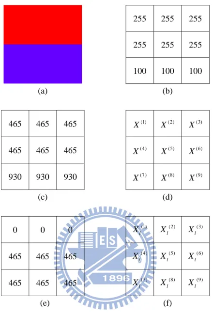
belongs to one of the vectors X_l(4) − X_l(9). Fig. 3.1 illustrates a simple edge example of the orderings of vectors based on the aggregate distances and the local sum of distances by the R-component only. Notice that the pixel in the center of the window has a smaller response of the aggregate distance in Fig. 3.1(c) denoted as X(5) in Fig. 3.1(d), and has a larger response of d m n_l

(

,

)

in Fig. 3.1(e) denoted as X_l(5) in Fig. 3.1(f).

255 255 255 255 255 255 100 100 100 (a) (b) 465 465 465 465 465 465 930 930 930 (1) X X(2) X(3) (4) X X(5) X(6) (7) X X(8) X(9) (c) (d) 0 0 0 465 465 465 465 465 465 (1) l X (2) l X (3) l X (4) l X X_l(5) X_l(6) (7) l X X_l(8) X_l(9) (e) (f)

Fig. 3.1. A simple edge example. (a) single edge image, (b) R-component values in edge area, (c) the aggregate distances, and (d) sorted pixels vectors corresponding to the same ordering of the aggregate distances, (e) the local sum of distances, and (f) Sorted pixels vectors corresponding to the same ordering of the local sum of distances.

Next, the edge detector Maximal Delta (MD) is defined as

(

)

(

( )

)

max , _l j ,

MD = F m n − X 4 ≤ j ≤ (12) 9

distances d i j_l

( )

, , the positions of these ordered vectors could also be edge candidates. Because that an edge is two pixels wide in nature, it suggests that we can find the maximum variation existent in the two pixels of edge bank by utilizing MD edge detector.

3.2 PCA based Color Edge Detection

3.2.1 YCbCr Color Space

Before we introduce our PCA based color edge detection, we now briefly introduce YC C color space. _{b r}

The color space of YC C can divided into luminance component (Y), and two _{b r} chromatic blueness component (C ), redness component (_b C ). _r C and _b C are the _r difference of blue and the difference of red chromatic components. The following conversion matrix is used to convert RGB color space into YC C color space. _{b r}

⎪ ⎩ ⎪ ⎨ ⎧ − × = − × = × + × + × = ) ( 7132 . 0 ) ( 5674 . 0 1145 . 0 5866 . 0 2989 . 0 Y R C Y B C B G R Y r b (13)

For a color edge detector, the goal is to detect edges that have changes in luminance or in chrominance. Our PCA based edge detection involves the reconstruction of the input image. We have to retain both chrominance and luminance information via the essential principal components of input image. Therefore, YC C _{b r} color space is selected in our PCA based color edge detection theme.

3.2.2 Eigencolor Image Construction

For an input image F of size M × N, each pixel location

(

m n,

)

is represented by a three-tuple color space vector F m n

(

,

)

for m =1, 2,...,M and

1, 2,..., .

n = N Each component of the color space in pixel location

(

m n,

)

can be represented as F m n_i

(

,

)

, for i =1, 2, 3. A color component of input image F is

denoted as F Then, for the color component_i. F the estimate of the mean is _i, calculated as

(

)

1 1 1 , M N i i m n M F m n M N = = = ×

∑∑

(14) For i =1, 2, and 3, M_i is expanded to a matrix F_i of size M × N having the value of M_i for every entry of matrix F_i. The covariance matrix estimate for the color component is

(

)(

)

T

i i i i i

C = F − F F − F (15) Next, we compute for matrix C eigenvalues _i's λ with _ij, V_ij being the corresponding eigenvectors such that λ_i1 ≥ λ_i2 ≥ ... ≥ λ_ij, for j =1, 2, ..., ,L where

(

)

min , .

L = M N We select the first k terms and the last _i k terms of eigenvectors _i

ij

v to retain the low frequency and the high frequency contents of the color image

.

F To obtain the compressed image for edge detection, we have to keep not only the low frequency principal components but also the high frequency components for detail and edge preservation, which is quite different from the conventional image

data compression approach. These eigenvectors are arranged in a matrix

1, 2, ..., _i, ( _i), ( _i 1), ..., .

i i i ik i L k i L k iL

E = ⎣⎡V V V V ₋ V _{− +} V ⎤_⎦

After obtaining the eigenvectors, we are now constructing an image called “eigencolor” image. First, the matrix F of the color component i is obtained by _i'

F_i' = F_i − F_i (16) And the weighting coefficients matrix W of selected eigenvectors can be computed _i

by

W_i = E F_iT _i' (17) The i-th color component is then constructed by

Eigen_i = E W_{i i} + F_i (18) The other two color components are also constructed in the same procedure.

Finally, the eigencolor image can be obtained by combining three constructed color components Eigen with the corresponding dimension order. _i

3.2.3 Edge Response Calculation

To obtain the edge response of the compressed eigencolor image, we simply apply the Sobel operator, as shown in Fig. 2, to each color component of eigencolor image, Eigen , and calculate the magnitude of edge response for each pixel location _i

( , )

(

,

)

2

(

,

)

2, 1, 2, ..., , 1, 2, ..., i i i h v ME m n = g m n + g m n m = M n = N (19) where ( , ) i h g m n and ( , ) i v

g m n are respectively the horizontal and vertical responses of the Sobel operator, shown in Fig. 3.2, in pixel location

(

m n,

)

for the i-th

component. +1 0 -1 +2 0 -2 +1 0 -1 +1 +2 +1 0 0 0 -1 -2 -1 (a) (b) Fig. 3.2. Sobel operator. (a) horizontal derivative approximation ,

i h g (b) vertical derivative approximation . i v g

By using a threshold T the _i, E function classifies the _i ME pixels into two _i

classes: edge pixels and non edge pixels as - ,

(

)

(

)

(

)

1 (edge pixel), if , , 0 (nonedge pixel), if , i i i i i ME m n T E m n ME m n T ⎧ ≥ ⎪ = ⎨ _< ⎪⎩ (20)

The edge image is obtained by a majority vote fusion rule on the detected edge of three color components. Let count denote the number that E m n_i

(

,

)

classifies pixel

(

m n,

)

as an edge for i =1, 2, and 3. Namely pixel

(

m n,

)

is classified as an edge if it is classified as an edge by at least two of its three color components, shown in (20). Otherwise, it is classified as a non-edge pixel and E m n

(

,

)

is set to 0.

(

,

)

1 (edge pixel), if 2 0 (nonedge pixel), otherwise

count E m n = ⎨⎧ ≥

⎩ (21)

3.3 Entropic Thresholding

To automatically obtain an optimal threshold that is adaptive to the image contents, the entropic thresholding technique is adopted. In the following, we illustrate how to apply entropic thresholding technique to the vector-order statistics based and the PCA based edge detections.

3.3.1 Entropic Thresholding for Vector-Order Statistics based Edge Detection

We are now introducing the entropic thresholding technique. Given a threshold, e.g., ,T the probability distributions for the edge and non-edge pixel classes can be

defined, respectively. As they are to be regarded as independent distributions, the probability for the non-edge pixels in a S ×S window having S pixels 2 P i_n

( )

can be defined as ( ) n₂ n l P i S = (22) where l indicates the number of pixels in the window that have the edge responses _n

smaller than or equal to threshold T . The probability for the edge pixels P i_e

( )

can be defined as ( ) e₂ e l P i S = (23)

where l indicates the number of pixels in the window that have the edge responses _e

greater than threshold T . The entropies for these two pixel classes are then given as

H_n

( )

T = −P i_n( ) logP i_n( ) (24)

H T_e

( )

= −P i_e( ) logP i_e( ) (25) The local optimal threshold T_l∗ selected for performing the non-edge and edge pixel classification has to satisfy the following criterion function:

( )

(

( )

( )

)

1, , 2 ..., max L l _{T T T T} n e H T∗ H T H T = = + (26) where T T₁, , ₂ ..., T are the proportional ratio constants with respect to the norm of _L

the mean vector of two sides (larger and smaller side) of the edge. In this way, the local optimal threshold T_l∗ reflects the relative magnitude variation with respect to the mean magnitude of current processing area. In our experiments, we select

1, , 2 ..., L

T T T to be 0.2, 0.3, ..., 0.9.

3.3.2 Entropic Thresholding for PCA based Edge Detection

After obtaining the magnitude of edge response E Sec. 3.2.2, of each color _i, component for pixels in the image, we introduce the entropic thresholding technique globally. We utilize all the Sobel edge response values of pixels in the input image as the possible choices of the global optimal threshold T_g∗ for each components .i For the i-th component of the color space, let the edge responses of the pixels have the range [0, ]h (the possible choices of the global optimal threshold), the probability _n

for the non-edge pixels in a M × N image P i_n

( )

can be defined as ( ) n , n l P i M N = × (27)

where l indicates the number of pixels in the input image that have the edge _n

responses smaller than or equal to threshold T. The probability for the edge pixels

( )

e P i can be defined as ( ) e , e l P i M N = × (28)

where l indicates the number of pixels in the input image that have the edge _e

responses greater than threshold T.

The entropies H_n

( )

T and H T_e

( )

for these two pixel classes can be computed according to Eqs. (23) and (24). The global optimal threshold T_g∗ selected for performing the non-edge and edge pixel classification has to satisfy the following criterion function:

( )

(

( )

( )

)

1 0, , max..., _n g _{T h h} n e H T∗ H T H T = = + (29)

However, the global optimal threshold T_g∗ will be too small and too sensitive for edge detection because that most pixels in the input image are non-edge pixels causing a bias leaning to the non-edge pixels’ edge strength. From Eq. (28), it is clear that maximum entropy occurs when the numbers of pixels in edge class and non-edge class are equal. Since most pixels are non-edge pixels, which have small magnitudes of edge response, T_g∗ naturally is tuned to a small value among the pixels’ edge response, which results in an erroneous edge/non-edge threshold selection. Therefore, we need to discard the pixels with small magnitudes of edge response in order to

alleviate the bias caused from the usual uneven distribution between edge pixels and non-edge ones. To solve this, we introduce a sensitivity parameter γ, which is automatically calculated from the input image content. The pixels which have the magnitudes of edge response smaller than the sensitivity parameter γ are the

obvious non-edge pixels and are discarded when applying our global entropic thresholding technique. On testing various images, we have found that the Sobel edge responses of obvious non-edge pixels usually have strengths smaller than five. To this end, we calculate the histograms of the edge response in the following ten intervals:

(

0, 0.5 , 0.5, 1 , ..., 4.5, 5 .

]

(

]

(

]

The value of γ is chosen to be the larger boundary of the interval that has the largest drop in histogram value, which could be the boundary for the obvious non-edge pixels and possible non-edge pixels. This is because that the majority of pixels in an image belong to non-edge regions and these pixels have small yet compact magnitudes of edge response. Therefore, we can assume that the intervals with maximal drop in histogram values represent the possible boundary between obvious non-edge pixels and possible non-edge pixels and we set γ to be the right boundary value of this interval. For example, if the maximal drop in histogram values of pixels’ edge strength occurs between

(

2, 2.5

]

and

Chapter 4 Experimental Results

In chapter 4, we test our vector-order statistics based and PCA based edge detection techniques on synthetic images and real world images. The synthetic images include one image that contains nine different color blocks with the same intensity. These synthetic images are generated for assessing the performance comparison. For all the real world images are smoothed by the Gaussian filter with σ =1 to alleviate the interference from noises. In the end of this chapter, we evaluate our edge detection techniques quantitatively by using Pratt’s Figure Of Merit (FOM) [24] and TPR, TNR and ACC of Receiver Operating Characteristic (ROC) [25].

4.1 Vector-Order Statistics based Edge Detection

We utilize our vector-order statistics based edge detectors to compute edge response and entropic thresholding technique to determine a local optimal threshold

.

l

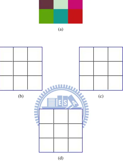
T∗ The first image we test on is a image consisting of 9 different color blocks with the same intensity as shown in Fig. 4.1(a). This image is applied to verify that our edge detection techniques works when objects in image has the same intensity but different hues. Figs. 4.1(b)−(d) show the edge detection results obtained by VMD, VDD and MD, and proves that our edge detection techniques can work under this circumstance. Fig. 4.2 gives the corresponding histograms of local optimal threshold

l

T∗ of VMD, VDD and MD to Fig. 4.1(a), where the X-axis is the proportional ratio constants described in Sec. 3.1.1.

(a)

(b) (c)

(d)

Fig. 4.1. Edge detection results of a color image with the same intensity. (a) original image, (b) edge detection by VMD, (c) edge detection by VDD, (d) edge detection by MD.

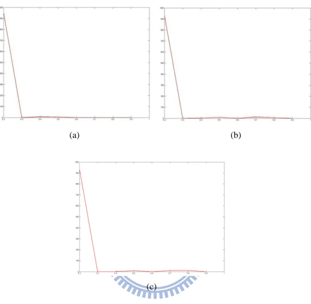
(a) (b)

(c)

Fig. 4.2. The corresponding histograms of local optimal threshold T_l∗ to Fig. 4.1(a). (a) histogram of T_l∗ using VMD, (b) histogram of T_l∗ using VDD, (c) histogram of

l

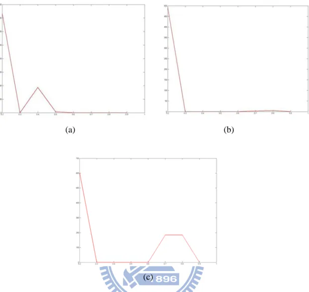
Next, we apply our edge detection techniques to images similar to Fig. 4.1(a) but with different intensities as shown in Fig. 4.3(a) and Fig. 4.5(a). Figs. 4.3(b)−(d) and Figs. 4.5(b)−(d) illustrate the edge detection result applying VMD, VDD and MD to Fig. 4.3(a). Fig. 4.4 and Fig. 4.5 give the corresponding histograms of local optimal threshold T_l∗ of VMD, VDD and MD to Fig. 4.3(a) and Fig. 4.5(a) respectively.

(a)

(b) (c)

(d)

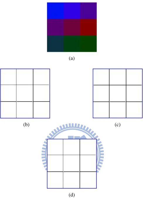
Fig. 4.3. Edge detection results of a color image with different intensities. (a) original image, (b) edge detection by VMD, (c) edge detection by VDD, (d) edge detection by MD.

(a) (b)

(c)

Fig. 4.4. The corresponding histograms of local optimal threshold T_l∗ to Fig. 4.3(a). (a) histogram of T_l∗ using VMD, (b) histogram of T_l∗ using VDD, (c) histogram of

l

(a)

(b) (c)

(d)

Fig. 4.5. Edge detection results of a color image with different intensities. (a) original image, (b) edge detection by VMD, (c) edge detection by VDD, (d) edge detection by MD.

(a) (b)

(c)

Fig. 4.6. The corresponding histograms of local optimal threshold T_l∗ to Fig. 4.5(a). (a) histogram of T_l∗ using VMD, (b) histogram of T_l∗ using VDD, (c) histogram of

l

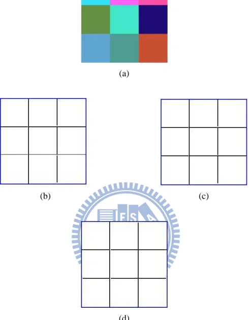
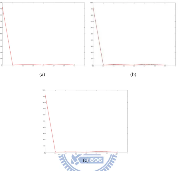
From the above results, our vector-order statistics based edge detection techniques are capable of detecting vertical and horizontal edges. Therefore, we are interested in their ability to detect diagonal edges. Fig. 4.7 shows the result of applying our edge detection techniques to an image with diagonal edges. Fig. 4.8 shows the corresponding histograms of local optimal threshold T_l∗ of VMD, VDD and MD to Fig. 4.7(a). At last, we apply our techniques to real world images, as shown in Fig. 4.9(a) and Fig. 4.10(a). The edge detection results are given in Figs. 4.9(b)−(d) and Figs. 4.10(b)−(d).

(a)

(b) (c)

(d)

Fig. 4.7. Edge detection results of a color image with diagonal edges. (a) original image, (b) edge detection by VMD, (c) edge detection by VDD, (d) edge detection by MD.

(a) (b)

(c)

Fig. 4.8. The corresponding histograms of local optimal threshold T_l∗ to Fig. 4.7(a). (a) histogram of T_l∗ using VMD, (b) histogram of T_l∗ using VDD, (c) histogram of

l

(a)

(b) (c)

(d)

Fig. 4.9. Edge detection results of a real world image. (a) original image, (b) edge detection by VMD, (c) edge detection by VDD, (d) edge detection by MD.

(a)

(b) (c)

(d)

Fig. 4.10. Edge detection results of a human face image. (a) original image, (b) edge detection by VMD, (c) edge detection by VDD, (d) edge detection by MD.

4.2 PCA based Edge Detection

Here, we test our PCA based edge detection technique. If an input image has size ,

M × N we select the minimum between M and N, as mentioned in Sec. 3.2.2., to be L. We select k_i to be 16% of L for Y color component and 8% of L for

b

C and C components. In Sec. 3.2.2., _r k_i represents how many eigenvectors we select to retain the low and high frequency contents of an input image. After we obtained the eigencolor image, Sobel operator is applied to obtain edge responses. The global entropic thresholding technique is then applied to generate the global optimal threshold T_g∗. The sensitivity parameter γ is generated automatically to facilitate the global entropic thresholding technique.

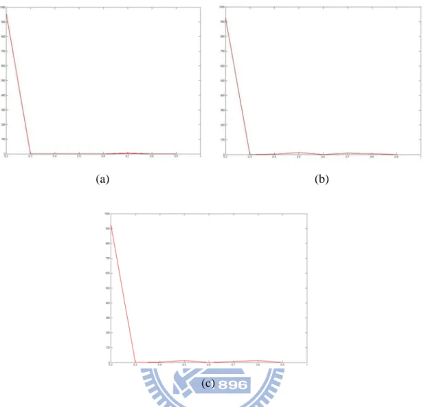
We first apply the image in Fig. 4.1(a) to test our PCA based edge detection technique, as shown in Fig. 4.11(a). Fig. 4.11(b) shows the corresponding eigencolor image in RGB color space. Fig. 4.11(c) is the corresponding edge detection result. From Fig. 4.11(b), we can observe that PCA can capture the low and high frequency image contents. Fig. 4.12 and Fig. 4.13 show the results of applying PCA based edge detection techniques to the color images in Fig. 4.5(a) and Fig. 4.7(a). Fig. 4.14 shows the probability density function (PDF) plots and cumulative distribution function (CDF) plots of T_g∗ taking the image with diagonal edges as an example. We can observe clearly that the maximum of entropy occurs when the numbers of pixels in edge class and in non-edge class are equal.

At last, we apply our techniques to real world images, as shown in Fig. 4.15(a) and Fig. 4.16(a). Fig. 4.15(b) and Fig. 4.16(b) show the corresponding eigencolor images in RGB color space. Fig. 4.15(c) and Fig. 4.16(c) are the corresponding edge detection results.

(a)

(b) (c) Fig. 4.11. Edge detection result of a color image with the same intensity. (a) original

(a)

(b) (c) Fig. 4.12. Edge detection result of a color image with the different intensities. (a)

original image, (b) the eigencolor image in RGB color space, (c) the edge detection result.

(a)

(b) (c)

Fig. 4.13. Edge detection result of a color image with diagonal edges. (a) original image, (b) the eigencolor image in RGB color space, (c) the edge detection result.

(a) (b)

(c) (d)

(e) (f) Fig. 4.14. The PDF and CDF of T_g∗ of the color image with diagonal edges. (a) PDF

of Y, (b) CDF of Y (CDF of T_g∗=0.499), (c) PDF of C , (d) CDF of _b C (CDF of _b

g

(a)

(b) (c) Fig. 4.15. Edge detection result of a real world image. (a) original image, (b) the

(a)

(b) (c) Fig. 4.16. Edge detection result of a human face image. (a) original image, (b) the

4.3 Comparing the Experimental results

First, we would like to introduce Pratt’s Figure Of Merit (FOM) and TPR, TNR and ACC of Receiver Operating Characteristic (ROC) as performance measures. FOM is defined as

{

}

_{( )}

2 1 1 1 100% max , ₁ D I i D I _i FOM I I = α _d = × +

∑

(30) where I and _D I are the number of detected and number of ideal edge points _I

respectively, α >0

( )

is a calibration constant, and d is the edge deviation for the _i th

i detected edge pixel. In all cases 0 < FOM ≤ for a perfect match between the 1; detected and the ideal edges FOM =1 whereas the detected edges deviate more and more from the ideal ones FOM goes to zero. The scaling constant α = 1₉ proposed in [14] has been adopted. Next, True Positive Rate (TPR) is defined as

(

TP

)

100%

TPR

TP FN

= ×

+ (31)

where TP (true positive) represents the number of pixels which are detected as an edge pixel and belong to an ideal edge pixel, and FN (false negative) represents the number of pixels which are detected as an non-edge pixel but belong to an ideal edge pixel.

On the other hand, true negative rate (TNR) is defined as

100% TN TNR TN FP = × + (32)

where TN (true negative) represents the number of pixels which are detected as an non-edge pixel and belong to an ideal non-edge pixel, and FP (false positive) represents the number of pixels which are detected as an edge pixel but belong to an

ideal non-edge pixel.

At last, accuracy (ACC) is defined as

100% TP TN ACC P N + = × + (33)

where P (positive) represents the total number of ideal edge pixels, and N (negative) represents the total number of ideal non-edge pixels. We also calculate the normalized

accuracy by

100% 2

TPR TNR

NACC = + × (34) The performance of our automatic color edge detection techniques are compared to those by color Canny edge detector [1], MVD edge detector [14], directional operator [15], Dikbas et al. [18], and automatic isotropic color edge detector [9]. Figs. 4.17−4.19 show the edge detection results of synthetic images for comparison. Tables I−III show the corresponding FOM, TPR, TNR, ACC and NACC of various edge detection schemes, with the script representing the rank of the method, of Figs. 4.17−4.19. From Tables I−III, we can see that our edge detection techniques perform well compared to other edge detection techniques. Figs. 4.20 and 4.21 show the edge detection results of real world images for comparison.

From the above results, we can see that our techniques perform consistently well compared to other edge detection techniques. Comparing the results by our PCA based technique with the results by automatic isotropic color edge detector, we can see that our global entropic thresholding technique performs better because that the sensitivity parameter γ alleviates the bias leaning to the non-edge pixels’ edge strength, which is mentioned in Sec. 3.3.2. The results of automatic isotropic color edge detector are too sensitive because that the edge detector utilizes all the pixels’ edge responses to determine the optimal threshold without alleviating the bias caused

from dominant non-edge pixels in number. From the results of our vector-statistics based edge detectors, VDD edge detector is more capable of alleviating the influence from noises but is too insensitive to real edges because that VDD detector discards the outlier X(9) while calculating the edge response. In general, MD detector is sensitive to small texture variation since it detects the genuine local maximal variance within the processing area.

(a)

(b) (c)

(d) (e)

(h) (i)

(j)

Fig. 4.17. Edge detection result of a color image with the same intensity. (a) original image, (b) VMD, (c) VDD, (d) MD, (e) eigencolor, (f) color Canny, (g) MVD, (h) directional operator, (i) Dikbas et al. [18], (j) automatic isotropic color edge detector.

(a)

(b) (c)

(d) (e)

(h) (i)

(j)

Fig. 4.18. Edge detection result of a color image with the different intensities. (a) original image, (b) VMD, (c) VDD, (d) MD, (e) eigencolor, (f) color Canny, (g) MVD, (h) directional operator, (i) Dikbas et al. [18], (j) automatic isotropic color edge

(a)

(b) (c)

(d) (e)

(h) (i)

(j)

Fig. 4.19. Edge detection result of a synthetic color image. (a) original image, (b) VMD, (c) VDD, (d) MD, (e) eigencolor, (f) color Canny, (g) MVD, (h) directional operator, (i) Dikbas et al. [18], (j) automatic isotropic color edge detector.

(a)

(b) (c)

(d) (e)

(h) (i)

(j)

Fig. 4.20. Edge detection result of a real world image. (a) original image, (b) VMD, (c) VDD, (d) MD, (e) eigencolor, (f) color Canny, (g) MVD, (h) directional operator, (i) Dikbas et al. [18], (j) automatic isotropic color edge detector.

(a)

(b) (c)

(d) (e)