職業及產業特性對台灣勞工長工時選擇的影響

行政院國家科學委員會補助專題研究計畫成果報告

期末報告

職業及產業特性對台灣勞工長工時選擇的影響

計 畫 類 別 ： 個別型計畫 計 畫 編 號 ： NSC 101-2410-H-004-029- 執 行 期 間 ： 101 年 08 月 01 日至 102 年 10 月 31 日 執 行 單 位 ： 國立政治大學經濟學系 計 畫 主 持 人 ： 李浩仲 計畫參與人員： 博士後研究：陳晏羚 報 告 附 件 ： 出席國際會議研究心得報告及發表論文 處 理 方 式 ： 1.公開資訊：本計畫可公開查詢 2.「本研究」是否已有嚴重損及公共利益之發現：否 3.「本報告」是否建議提供政府單位施政參考：否

中 華 民 國 103 年 01 月 29 日

中 文 摘 要 ： 不同的產業及地區其勞工的工時選擇有很大的差異，因此本 研究計畫所要問的問題是：為什麼不同產業或不同地區間的 勞工其有不同的工時決策？這是否是因為各產業（地區）有 不同的發展軌跡，導致其內的勞工工時選擇有所不同？為了 解答以上的問題，我們建構了五項產業（地區）特性指標： 長工時溢酬、所得不均度、雇用人數成長率、平均薪資、及 部份工時勞工比例，並分別探討其對工時的影響。 我們的結果顯示，產業（地區）所得不均度對於長工時有顯 著的正向影響，此一結論符合 Bell and Freeman (1995)的 看法：由於勞工預期增加工時有助於其未來前景，薪資不均 度擴大會使工時增加的邊際利益上升，進而鼓勵勞工增加工 時；概念相似地，我們亦發現地區長工時溢酬會增加工時， 但產業長工時溢酬的影響卻為負向或不顯著，我們認為這可 能是由於有勞工流動性問題使從產業的角度分析有其侷限 性。我們同時發現部份工時勞工比例和工時有顯著負向關 係，我們推論高部份工時勞工可能反應著該產業或地區允許 較彈性的工作型態，因此其勞工不需大量投入時間在工作 上；我們尚看到部份證據顯示雇用人數成長率和工時呈負相 關，我們認為這反應工作保障為讓勞工不需要超時工作；最 後，亦有證據顯示平均薪資和工時呈正相關，這意味著薪資 上升的替代效果大過所得效果。考量多數勞工薪資並不算 高，這樣的結果符合預期。 中文關鍵詞： 工時, 長工時溢酬, 不均度, 部份工時勞工比例 英 文 摘 要 ： 英文關鍵詞：

1

國科會計畫期末報告：職業及產業特性對台灣勞工長工時選擇的影響

計畫編號：NSC 101-2410-H-004-029

計畫主持人：政治大學經濟系李浩仲

論文題目：

產業及地區特性對台灣勞工長工時選擇的影響

1

I. 序論

台灣勞工的長工時問題在近年來愈發受到社會矚目，勞工過勞發生不幸的消息 也屢屢成為新聞議題。根據主計總處以及勞委會統計顯示，台灣 2012 年平均每名勞工 工作 2140.8 小時，工時全球第 3 高，和許多東亞國家一樣均屬於長工時國家。 然而另一方面，台灣勞工的平均工時在過去三十多年來其實是下降的。例如， 根據行政院主計處人力資源調查顯示，台灣就業者在 2000 年時每人每週平均工時是 46.09 小時，但在 2010 年卻是 43.60 小時。這當中一個重要因素，就是在 2001 年時台 灣全面實施週休二日。或許職是之故，台灣經濟學界近年的文獻主要討論的反而是 “縮短”工時所帶來的各種層面影響，或是台灣近年非典型就業或是失業的問題。2 _相 對來說，對於台灣勞工為什麼會需要那麼長的工時，以及那些外在環境因子會影響勞 工的工時選擇，文獻上卻少有討論。本計劃的目的即是從此一重要的面向進行探討， 希望能對台灣勞工工時的研究有所補充。 本文想要嘗試回答的問題是：為什麼不同產業或不同地區間的勞工其有不同的 工時決策？這主要是來自於各產業（地區）勞工本身特質的差異，抑或是因為各產業 （地區）有不同的發展軌跡，導致各產業（地區）工時的不同？ 近期國外文獻強調， 人們的工時選擇不只著眼於工時長短對現在所得的影響，亦重視現在工時對未來所得 的影響。因此各產業或地區間如果其工時所帶來的未來報酬不同，則其勞工的平均工 時亦可能不同。奠基於此一觀點，本計畫建構了三個不同的產業（地區）特性的指標 來衡量各產業（地區）間當下工時所可能帶來的未來報酬差異：產業（地區）長工時 溢酬；產業（地區）內所得不均度；和產業（地區）內雇用人數成長率。在這三項指 標當中，前兩項指標的建立主要立基於 Bell and Freeman (1995)和 Kuhn and Lozano

1 _{原申請題目為職業及產業特性對台灣勞工長工時選擇的影響。在研究過程中本研究發}

現地區特性扮演更重要角色，故將主要視角轉向地區及產業特性。

2 _{關於縮短工時問題，如徐美、陳明郎(2011)。關於非典型就業問題，如江豐富}

2 (2008)的看法：在勞工預期提高工時會幫助其未來薪資前景的狀況下，產業（地區） 內的薪資不均度擴大意味著工時增加的邊際利益會上升，進而鼓勵勞工增加工時；最 後一項指標則是試圖衡量勞工所面對的工作不穩定程度之負面指標。我們想瞭解當勞 工感受到其工作有不穩定的情況下，其可能的工時選擇改變。然而在此需理解的是， 儘管當工作不穩定程度提高時勞工或有意願增加工時以避免遭到裁員，但廠商不一定 願意讓勞工超時工作，因此工作不穩定程度和工時之間在理論上並沒有確切的關聯。 除了從長期所得的角度探討不同產業（地區）其長工時的成因，本計劃另外探 討兩種產業（地區）特性對工時的影響：產業（地區）平均薪資及部份工時勞工比例。 薪資和工時之間的關係是傳統勞動供給理論的核心，其中薪資所造成的所得及替代效 果對工時的影響相反，因此兩者之間的關聯主要是一個實證問題。部份工時勞工比例 和工時之間的關係從理論上也難以界定。一方面高比例的部份工時勞工可能反應著該 產業（地區）允許較彈性的工作型態，因此不需要勞工投入大量工時在工作上，另一 方面也可能意味著該產業（地區）面臨衰退，原本全職勞工轉成兼職勞工，因此勞工 反而可能增加工時以保障其工作。我們將嘗試透過資料瞭解其實際影響。 我們的結果發現，從歷史趨勢而言台灣長工時的比例在 1978-2012 年間是下降的， 但自 2001 年後此一比例反而略有緩步向上的情形。我們亦發現不同教育程度者，不同 產業，及不同地區的勞工，其長工時比例變化明顯不同。例如說，我們發現低教育程 度、傳統製造業、鄉鎮地區的勞工其工時是快速下降的，但高教育程度、電子、金融、 法律服務業、及大都會地區勞工其工時反而自 1990 年代後有上升的情形。如何解釋這 些產業及地區間的差異？透過我們建構前述產業及地區性特性指標，我們發現產業 （地區）所得不均度對於長工時有顯著的正向影響，而地區內長工時溢酬也會增加工 時；此外，我們亦有證據顯示平均薪資和工時呈正相關，這意味著薪資上升的替代效 果大過所得效果。最後，我們發現部份工時勞工比例和雇用人數成長率皆與工時有顯 著的負相關性。 本結果報告接下來的安排如下：第二節我將進行文獻回顧；第三節將介紹台灣 勞工工時的演進；接下來第四節我將依序提出資料的建構、實證模型、及實證結果和 討論；最後一節我將為本報告做一總結並探討接下來研究的方向。

3

II. 文獻回顧

在傳統經濟學模型裡，勞工面對的勞動－休閒之間的抉擇主要取決於兩大要素。 首先，勞工對於勞動有其特殊偏好：有些勞工可能視工作為人生樂事，有些勞工則視 工作為畏途；其二，勞工的勞動（工時）選擇也可能取決於其他外在的誘因，例如薪 資等。一般認為，勞工對於勞動的偏好和其教育程度、年齡、性別，或擁有的非薪資 所得等個人因素相關；而薪資對於勞工工時的選擇則同時存在替代及所得效果。替代 效果意味著勞工願意因為薪資提高而花更多時間工作，而所得效果則意味著當薪資 （所得）提高時勞工希望會多休閒（因為休閒為正常財）而減少工作。實證結果大致 上認為替代效果在低所得狀況下較明顯，而所得效果會在所得提高的過程中愈顯重要 (Drago, Black, and Wooden, 2005)。

然而除了上述傳統的經濟學模型從偏好及薪資誘因等面向解釋工時，近年來的 工時研究則嘗試尋找其他解釋。首先，有些文獻強調“當下”工時的長短對“未來”薪資 的高低會有影響，因此勞工在選擇工時時會將這些長期因素一併考量。例如說， Michelacci and Pijoan-Mas (2007)認為勞工可能選擇較長工作時間是因為工時提升會提 高其人力資本，幫助其在未來取得升遷的機會。另一方面，Akerlof (1976)則強調勞工 可能寧願長時間待在工作崗位上以顯示(signal)其較高的生產力；例如在實證上， Landers et al (1996)發現在美國律師事務所資深律師會以工作時間來評斷年輕律師的適 任性，而年輕律師會因而選擇長時間的工作；類似的，Rosenthal and Strange (2008)利 用美國 1990 年橫斷面各職業的資料發現年輕專業人士會因為有競爭對手的存在而提高 其工作時間，而這在人口眾多的大城市裡尤其明顯。3_{此外，Bluestone and Rose (1998)}

則認為當勞工認為其所進行的工作是不穩定的時候，其會較長時的工作以減少被裁員 或減薪的可能性。

奠基於上述的看法，有部份研究則進一步探究勞動市場特性如何影響工時的選 擇。Bell and Freeman (1995)認為薪資不均會使得勞工增加其工時，這是因為勞工增加 工時會提高其未來薪資前景，而這個未來薪資的提高量會因為薪資不均程度的提高而 增加。Bell and Freeman (2001)研究德國和美國長期追踪資料發現，無論是在德國或美 國，薪資不均程度越高的職業其工時越長，且長工時對未來薪資及升遷都有正向影響。 另外，由於自 1970 至 1997 年這三十年間美國的不均度增加情形遠超過德國，所以他 3 _{相反地，他們發現非專業人士沒有這種現象－當做同類型工作人數眾多時，非專業人} 士的工時會減少。他們認為這是因為非專業人士之間較沒有競爭關係，所以在同類型 工作人數眾多時會選擇工作分攤而降低工時。

4

們觀察到同一段時間內德國勞工的工時減少，但美國勞工的工時卻增加。類似地， Kuhn and Lozano (2008)利用美國 Current Population Survey 發現美國自 1970 至 2006 年 間美國的高薪、高教育、及年長的領固定薪水勞工其工時增加愈多，而其主因是在於 這些勞工服務的產業及從事的職業其不均度提升且長工時的溢酬(premium)較高；至於 Michelacci and Pijoan-Mas (2007) 則是研究美國和歐盟的資料。他們除了同樣發現不均 度提高會增加工時外，亦發現當勞動市場愈擁擠(tight)、生產力對人力資本的彈性愈大 時，工時愈會增加。這些結果均呼應前面所提文獻的看法。

前述各研究主要是從工時所帶來的長短期所得來探討勞工工時的決策。然而， 另有研究是從 “消費主義＂的觀點來探討工時的選擇。Schor(1999)認為隨著新產品和 服務的出現，美國人，尤其是高社經地位的人，逐漸擴大維持最低生活水準的消費需 求，因此他們就必須要工作更長的時間，賺取更多的金錢支撐消費。Drago, Black, and Wooden (2005)觀察澳洲的資料發現這種消費主義是澳洲長工時工作人口增加最重要的 原因。Bowles and Park (2005)調查 OECD 國家 1963-1998 的資料發現在此樣本的國家

中，所得不均程度越高時，平均工時越長。他們的結果非常顯著且強健。4_{他們解釋他}

們的結果印證了 Veblen Effect：一個人的效用其中有一部份是根據個人和比較對象 (reference group)相對的消費水準決定的，而比較的對象則是社會裡社經地位高的人； 當所得不均程度越高，消費能力不均程度越高，而人們會為了達到更高的消費能力， 因此更加賣力的工作。另一個有趣的研究是 Carlsson, Johansson-Stenman, and

Martinsson (2007)，他們根據瑞典資料衡量人們對相對所得或某些商品的相對消費的感 覺。結果發現，人們會以所得高低來彰顯其地位，但不會以休閒時間來顯示地位－這 兩者都意味著人們願意為其社會地位投入較長的工時。 以上提到的各種觀點均是從勞動供給的角度來探討工時長短的問題，而不是從 勞動需求的角度來探討此一議題。其主要的原因是認為至少就長期而言勞動需求者需 配合勞工本身的工作意願來安排其工作(Golden, 2009)。然而，如果考量到雇用員工有 眾多固定成本（例如招募、訓練等成本），公司可能會選擇利用調整工時長短來因應 經濟景氣循環 (Golden, 1990)。 國內近年來探討工時議題的文獻主要著重在兩方面。第一，部份文獻主要在探 討在西元 2001 年週休二日工時縮短政策實施後，台灣經濟成長狀況及廠商行為是否有

4 _{Bowles and Park (2005)衡量的是一個國家的總體不均度指標（例如吉尼係數），而前}

面所提論文如 Bell and Freeman (1995)、Kuhn and Lozano (2008)等則是衡量“職業內＂ 或“產業內＂的不均度。

5 所改變。例如徐美、陳明郎(2010) 透過分量迴歸模型，以台灣整體產業和製造業中分 類資料，探討全面實施週休二日政策縮短工時對於各產業勞動生產力分配的影響。5_第 二，亦有部份文獻著重在探討台灣近年來非典型就業或工時彈性化問題，例如江豐富 (2011) 採用 2008 年 5 月行政院主計處「人力資源調查」暨附帶之「人力運用調查」的 個體資料, 並以兩階段估計法估計勞工從事典型與非典型工作的機率與工資率。6_這兩 類型的研究都探討了近來工時趨勢的重要面向，但對於長工時何以形成以及各職業或 各產業工時狀況的差異則較少觸及。部份文獻如陳淑芳(2007)將工時長短和個人特質 進行連結，然而其亦未探討產業、職業、甚至總體情勢對工時選擇是否有所影響。一 個例外是林向愷、岳俊豪(2009) ，他們利用 EGARCH-X 模型發現顯台灣自 2000 年每 人平均工時變異數增加，而貿易自由化可能是其背後成因。7 5_{徐美、陳明郎(2010)的結果顯示在週休二日工時縮短政策實施後，整體製造業相對服} 務業的勞動生產力顯著地提升，但其增加效果在勞動生產力分配各分量上是不一的， 而各製造業中分類產業所受到的效果也不一。另一方面，營造業相對於服務業之勞動 生產力在工時縮短政策實施後顯著減少，且在各分量減少的程度幾乎呈現一致。 6_{江豐富(2011)發現具有以下特徵的勞工，較可能選擇非典型就業：較低低教育程度} 者、各學歷的肄業者、女性青少年、一般市場經驗水準愈高者、主要工作場所的行業 不是製造業或營造業、受雇者、曾退休再重返勞動市場者 , 以及女性勞工、或男性且 是未婚或單親者、 女性且是已婚且配偶存在者。 7 _{變異數增加可能是因為長工時工作者增多，也可能是短工時工作者增多；這一部份他} 們沒有特別觸及。

6

III. 台灣勞工工時趨勢

全體受雇者樣本 下圖為 1978 年至 2012 年間一週工時超過 50 或 55 小時者的百分比，其樣本資料 來自行政院主計處人力資源調查，僅觀察受雇者，且一週工時大於 30 小時以上之樣 本。從下圖中，我們發現無論定義一週工時大於 50 或 55 小時為長工時，其趨勢皆非 常類似，因此接下來本文皆將以 50 小時定義為長工時。整體而言，我們觀察到長工時 者的比例在趨勢上是遞減的，然而這當中以在 1995 年以前減少的速度是最快的，而在 2001 年左右達到最低點。在 2001-2012 年間，長工時工作者的比例其實略有緩步增 加，於 2012 年長工時工作者約占整體受雇勞工的 13%。我國自 1998 年 1 月 1 日起施 行隔週休兩日，2001 年 1 月 1 日開始實施週休兩日，但觀察長工時者比例的變化趨勢， 我們並未觀察到這些政策實施對於長工時比例的減少有太大的助益。 性別 女性勞動參與率大幅提升是台灣勞動市場近三十年重要的變化之一，對於性 別間長工時比例之差異有討論的必要性，故我們於下圖再區分為男性樣本與女性樣 本進行觀察。以圖二的時間趨勢圖形觀察，男性長工時比例大於女性長工時比例， 並且男性與女性長工時者比百分比大致上時間變勢類似， 1978 年至 2001 年大致是 下滑的情況，而於 2001 年後是有回升的趨勢。有趣的是，我們看到男性與女性長 工時比例差異由 1978 年至 2001 年間逐漸縮小，2001 年兩者比例差距僅 2%，但 2001 年後兩者比例差距又再度提高，於 2012 年達 3.5%。

7 教育 在下圖中我們再依教育程度來區分觀察長工時者時間變化趨勢。我們發現國中以 下、高中與大專以上三種教育程度長工時者之百分比時間趨勢有著相當大的不同。國 中以下者，其長工時比例由 1978 年至 1997 年有著大幅下跌的趨勢，1998 年後則是略 有上升；高中程度者在 1978 年至 1997 年亦有著下跌的趨勢，惟其降幅明顯較國中以 下者較緩。高中程度者之長工時比例於 1978 年至 1997 年間明顯小於國中以下教育程 度者，但差異幅度是逐漸縮小，而於民國 1998 年後兩者比例差異微小，惟 2007 年後 其比例明顯超過國中程度以下者。大專以上教育程度者則與前兩者的時間趨勢有著明 顯之差異，其於 1991 年前大致上有微幅下降情況，並百分比明顯低於國中以下、高中 教育程度者，惟差距漸減。而在 1991 年後大專以上教育程度者長工時比例時間反而是 緩步上升，並於 2009 年超過國中程度以下者。 產業 接下來我們將討論產業間長工時比例的差異。圖四中我們區分產業，觀察成衣及 服飾品業、電子及電子業、金融業與法律及工商服務業長工時變化時間趨勢。我們發 現，不同產業其長工時比例有很明顯的改變趨勢。首先，成衣及服飾品產業偏向傳統 產業性質，發現其長工時比例較類似全體樣本的時間趨勢，大致呈現下滑的趨勢；其 次，電子及電力業的長工時比例在 2001 年之前也呈現下跌的趨勢，但之後便呈現長工 時者比例上升的情況，這應是近十數年多電子業興盛帶來之影響。金融業與法律及工

8

商服務業其長工時比例大略由 1991 年後即呈現上升的趨勢，但以法律及工商服務業成 長幅度較大。以這個項產業而言，金融業近三十多年的長工時比例變化幅度最小，另 外，近年法律及工商服務業與電子及電力產業之長工時比例有明顯上揚的趨勢。

9 地區 除了從產業別進行比例，我們於下圖針對不同縣市進行比較。有趣的是，我們發 現不同縣市其長工時比例軌跡有明顯不同的趨勢。比較南投縣及台北市，我們看到南 投縣長工時比例和全國的趨勢類似，但台北市則明顯不同。我們發現，從 1982 至 2012 年間台北市的長工時比例其實是長期緩和上升的，於 2012 年時達 16%，遠高於 全國平均的 13%。 小結 從以上的結果，我們看到整體而言台灣長工時的比例是下降的，但隨不同教育程 度者，不同產業，及不同地區，我們看到其趨勢變化明顯不同。因此一個自然而升的 問題，這些的差異根源是什麼？在接下來的實證分析裡，我們將特別著重討論產業及 地區特性業長工時差異的影響。

10

IV. 實證分析

IV.1 產業（地區）特性指標的建構 本計畫的主要重點是在探討產業及地區特性對於勞工工時選擇的影響。在本小節 中，我將依序說明我所探討的五個特性指標的意涵及建構方式。這些指標包含：產業 （地區）的長工時溢酬、所得不均度、雇用人數成長率、平均薪資、及部份工時勞工 比例等。建構特性指標的資料來源有二，首先是主計總處所進行的人力資源調查 1978-2012 的調查資料，其調查項目包括家戶內人口與就業相關的資訊，例如勞動狀態、工 時、職業別、行業別，及各項基本資訊 ，例如婚姻狀態、性別、年齡、教育、居住地 等。其次我將使用於每年五月進行人力運用調查，其原為一人力資源調查的附加調 查，但進一步提供了勞工薪資等相關資訊。我們所使用的樣本包含所有 15-64 歲之未 全時就學勞工。有鑑於台灣的產業類別分類曾有九次的修訂，為求理解各產業長時間 特性的演變，本研究有先將歷次產業編碼進行調合的動作，總計得 49 個產業。另外我 們亦有針對五都的形成調合行政區的編碼，總計 20 個縣市。 1. 長工時溢酬 我建構的第一項的指標是產業（地區）的長工時溢酬，此一指標主要是希望能捕 捉長工時所帶來的長期性效益，諸如較佳的升遷機會、較多的受訓機會等。理想上此 一指標的建立需要利用追蹤資料，然而由於台灣最主要的追蹤資料－華人家庭動態調 查於 1999 年後才展開，且樣本數不足以在較細的產業層級上進行分析，因此我的建構 方式主要是參照 Kuhn and Lozano (2008)透過橫斷面的人力運用調查來進行。接下來的 敍述將以產業長工時溢酬指標為例，地區長工時溢酬的計算和其類似，故不贅述。 針對於在 t 年於產業 j 工作的樣本 i 我們首先針對每一產業 j 分別進行下列迴歸： log⁡(rwage)_𝑖𝑗𝑡 = 𝛽_1𝑡𝑗ℎ𝑜𝑢𝑟_𝑖𝑡+ 𝛽_2𝑡𝑗 (ℎ𝑜𝑢𝑟_𝑖𝑡)2_{+ 𝛿}′_𝑿 𝒊𝒕+ 𝜽𝒕 其中，rwage為工作於 j 職業的個人 i 在 t 時間時的實質月薪，ℎ𝑜𝑢𝑟𝑖𝑡為每周平均 工作時間、(ℎ𝑜𝑢𝑟_𝑖𝑡)2_{為每周平工時平方、𝑿} 𝒊𝒕包含一系列個人控制變數，諸如年齡及其 平方、教育程度、年資及其平方、婚姻狀態等、而𝜽_𝒕為時間固定效果。根據上述迴歸 式，係數𝛽_1𝑡𝑗及𝛽_2𝑡𝑗 可以告訴我們薪資和工時之間的横斷面關係，我將如原本 Kuhn and Lozano (2008)論文定義職業內長工時溢酬為工作 55 小時的平均估算薪資和工作 40 小

11 時的平均估算薪資之間的差異。 在此要說明的是，雖然原則上我們可以針對每一產業每一年資料分別進行迴歸以 得到不同的𝛽_1𝑡𝑗及𝛽_2𝑡𝑗 計算長工時溢酬，實際在資料處理時考量樣本數問題針對每一年 的迴歸我將前後兩年的所有同一產業之樣本納入迴歸分析，並加上時間虛擬變數控制 不同年度景氣差異。例如說，如果要計算 1995 年的溢酬，我將 1993-1997 的資料納入 迴歸，而在計算 1996 年的溢酬時我則將 1994-1998 的資料納入迴歸。 2. 所得不均度

本計畫中測量產業（地區）所得不均度的指標是依照 Bell and Freeman (2001)的 方式來衡量 ，以產業（地區）內的實質薪資標準差來衡量。由於人力運用調查原為一 抽樣調查資料，我有依樣本的權重回推母體的所得不均度。此一指標同樣是希望能捕 捉長工時所帶來的長期性效益。如 Kuhn and Lozano (2008)所說，較大的所得不均度可 能源於獎勵方式的改變，也可能來自於不同廠商之間的給薪差異，這些皆會誘使勞工 增加工時以達到較好的地位。 3. 雇用人數成長率 此一指標的資料來源是人力資源調查，我先計算歷年各產業（地區）的勞工數， 再計算其成長率。此一指標的建立主要是希望捕捉一位勞工在職業上所面對的工作穩 定度：當此指標較高時，意味著該產業（地區）有在新增勞工，因此原本的勞工較沒 有失去工作的風險。 4. 平均薪資 此一指標的資料來源是人力運用調查，以產業（地區）內的平均實質薪資來衡 量。薪資的上升對工時選擇可能帶來負向的所得效果及正向的替代效果，是固我們將 觀察兩者之間的重要性差異。 5. 部份工時勞工比例 此一指標的資料來源是人力資源調查，我計算歷年各產業（地區）的部份工時勞 工佔全體勞工的比例。我定義部份工時勞工為每周工作不足 30 小時之勞工。高比例的 部份工時勞工可能反應著該產業（地區）允許較彈性的工作型態，也可能意味著該產

12 業（地區）面臨衰退，將原本全職勞工轉成兼職勞工。因此理論上我們無法推知其影 響方向。

IV.2 實證模型

本研究中，我首先將分別在產業（地區）層級探討產業（地區）對平均工時的 影響。我會先如上面所述計算產業（地區）的特性變數，並且算出各產業（地區）長 工時工作（我們在此定義 50 小時會長工時）勞工的比例，最後再觀察各特性變數和長 工時比例之間的關聯。具體而言，我將使用下列迴歸式進行分析： longhr_ratio_𝑗𝑡 = 𝛽′_𝑿 𝒋𝒕+ 𝜽𝒋+ 𝜽𝒕 在上式中，longhr_ratio𝑗𝑡代表產業（地區）j 在 t 年的長工時比例，𝑿𝒋𝒕代表產業 （地區）j 在 t 年的特性變數，𝜽_𝒋代表產業（地區）j 的固定效果，而𝜽_𝒕代表時間 t 的固 定效果。要注意的是，由於我們加了產業（地區）j 的固定效果，我們所估計的係數能 解釋同一產業（地區）其各年度長工時比例變化的原因，而非僅是橫斷面的關聯性分 析。 在此我們先探討此一迴歸式和文獻回顧所提到之影響工時因子間的對應關係。 從文獻中我們知道有許多因素可能影響工時決策，包含個人對工作的偏好、薪資的所 得及替代效果、增加工時的長期報酬、消費主義、景氣循環、以及其他總體環境因素 （例如全面執行週休二日、派遣及彈性工時的普及等）。在上述迴歸式中，加入主要 解釋變數𝑿_𝒋𝒕即為了從不同層面觀察增加工時的長期報酬可能對工時選擇的影響。針對 個人工作偏好以及薪資的所得和替代效果，我會對不同教育程度的子樣本分別進行迴 歸分析來進行控制。此外，為了考量消費主義、景氣循環、及政府政策等總體環境因 子的可能影響，我用時間固定效果加以考量。89 使用類似上式的產業（地區）分析是文獻上探討工時議題的常見做法，其主要 好處有二：第一，我們主要的解釋變數本身就是在產業（地區）層級上建構，因此在 8 _{徐美、陳明郎(2010)指出全面周休二日的實施對於服務業的影響較製造業的影響低，} 這意味著一個單純時間固定效果無法捕捉這一個現象。一個可行方法是讓服務業及製 造業有不同的時間固定效果。 9 _{加入縣市固定效果的另一個理由是能控制各縣市的物價差距。由於在迴歸模型中我無} 法加入（實質）薪資資訊，所以考慮縣市固定效果能部份控制生活成本對工時選擇的 影響。

13 同一層級進行迴歸分析也是一個自然的選擇。第二，如 Borjas (1980)所提出，在個人層 級討論勞動供給問題常面對 division bias 的問題，也就是說，由於問卷中的工時時數經 常有誤，因此估計結果亦會偏誤。另一方面，在產業（地區）層級上進行分析的缺點 在於其對於勞工特質未能仔細掌握，因此我亦進行下列個人層級的迴歸以進行比較。 我考慮以下個人層級的迴歸模型以探討產業（地區）特性和個人工時之間的關 聯。對一個在 t 時間、在 j 產業（地區）工作的 i 樣本而言，使用的迴歸式如下： log⁡(hour)𝑖𝑗𝑡 = 𝛽′𝑿𝒋𝒕+ 𝜹′𝒁𝒊𝒕+ 𝜽𝒋+ 𝜽𝒕+ 𝜺𝒊𝒋𝒕 . 其中，應變數log⁡(hour)_𝑖𝑗𝑡是 i 樣本每周主要工作時數的對數；𝑿_𝒋𝒕如前是產業 （地區）特性指標；𝒁𝒊𝒕為對每周主要工作時數有影響的個人特質變數，包括個人的年 齡及其平方、教育程度、婚姻狀況等；𝜽𝒋和𝜽𝒕如前代表產業（地區）及時間的固定效 果，𝜺_𝒊𝒋𝒕為誤差項。和前面產業（地區）分析比較，最主要的差異在我們可透過𝒁_𝒊𝒕對 個人特質進行控制，但可能要付出的代價在於會有 division bias 的疑慮。

IV.3 實證模型迴歸結果

產業層級迴歸結果分析 在表一中我們呈現了在產業層級上的迴歸結果分析，在第 (1)-(4)列我們呈現了 當定義長工時為 50 小時的結果，而在第 (5)-(8)列我們呈現了當定義長工時為 55 小時的 結果。先從第 (1)列觀察全體樣本的結果，我們有以下發現。首先，我們發現產業雇用 人數成長率對工時的影響是負向的，這和我們的期待一致。由於較高的雇用人數成長 率意味著原本業內的勞工的工作保障程度較高，因此其較沒有誘因特定從事長時間工 作。其次，我們發現部份工時勞工比例亦對工時的影響是負向的。從我們前面的討論， 這可能源於高部份工時勞工可能反應著該產業允許較彈性的工作型態，因此勞工不被 期待投入大量工時在工作上。第三，我們發現平均薪資和長工時呈正向關聯，這意味 著平均而言薪資上升所帶來的替代效果大過所得效果。考量台灣勞工薪資並不算高， 這樣的結果頗符合預期。第四，我們發現當產業內薪資標準差提高時，工時會上升。 這一個結果和 Bell and Freeman (2001)及 Kuhn and Lozano (2008)針對美國及德國資料所 做的分析一致，這意味著當所得不均度提高時，差異化的薪資會促使勞工更長時間的 工作。第五，和我們原本不一致的，我們發現長工時溢酬反而和工時呈負向關聯。這

14

一個結果和 Kuhn and Lozano (2008)的發現相類似，而我們將在後面地區層級分析及個 人層級分析時再特別討論其可能的因素。 如果我們針對不同教育水準的勞工進行比較，我們發現其結果和全體勞工的結果 非常類似，唯一的例外是產業雇用人數成長率對工時的影響不再顯著。此外一個有趣 的結果是所得不均度提高時對於低教育程度之勞工工時影響最大、中等教育程度者次 之、而高教育程度者最少。最後，如果比較第 (1)-(4)列及第(5)-(8)列，我們發現長工時 的定義對於我們的結果沒有差異。 地區層級迴歸結果分析 在產業層級上的分析時我們遇到兩個難以理解的結果。首先，我們發現長工時溢 酬和工時呈負向關聯。其次，我們發現當針對不同教育水準的勞工分別進行分析時， 產業雇用人數成長率對工時的影響不再顯著。這樣的結果其實可能反應著在產業層級 上進行勞動現象分析可能有其侷限之處。台灣的勞動市場是一個流動性高的勞動市場， 勞工可能會因為認定本身所處產業不具發展前景，或不滿意其工作條件而轉換工作， 因此如果當我們將分析層級定義在產業上，可能結果會因勞工的流動而有所失真。這 樣的論點在近期國際貿易對於勞動市場影響的研究逐漸受到重視，例如 Ebenstein et al. (2013)强調應當從職業層級進行分析，Autor, Dorn, and Hanson (2013)則强調應當從地區 層級進行分析。選擇職業或地區層級主要是著眼勞工不太容易轉換職業或居住地，因 此如果有任何的衝擊，其難以透過工作移動躲避衝擊。職是之故，我們於表二在地區 層級進行迴歸分析。 比較表一和表二，我們發現大部份的結果都維持不變，這意味著我們前面的結論 具有強健性。然而，就如我們期待的，當我們從地區層級進行迴歸分析時，我們發現 長工時溢酬和工時轉而呈正向關聯，雇用人數成長率對工時的影響除了高教育樣本外 也出現了期待中的負向顯著性，這些結果皆符合原本理論上的預期。 個人層級迴歸結果分析 如前所述，文獻裡對工時的分析主要是從產業或職業層級分析，較少從個人層級 探討，這主要是擔心 division bias 的問題。但另一方面，從個人層級探討較能針對個人

15 特質進行控制，因此我們利用表三及表四分別探討產業及地區特性對於工時選擇的影 響。和表一和表二略有不同的，我們現在的應變數是勞工的實際工時取其對數。 從表三及表四我們發現我們在之前觀察到的結論沒有太多改變，但顯著性有明顯 的差別。比較表一和表三，我們發現當我們探討產業特性的影響時，如果從個人層級 出發雇用人數成長率及平均薪資對工時的影響皆轉為不顯著，但所得不均度及產業部 份工時勞工比例的影響皆維持顯著性。比較表二和表四，我們發現當我們探討地區特 性的影響時，所有係數皆維持相同的影響方向，但顯著性上雇用人數成長率及平均薪 資的影響再次轉為不顯著，而長工時溢酬、所得不均度、及產業部份工時勞工比例仍 維持顯著性。 從上面的結果來看，有鑑於個人層級分析本身就有 division bias 的問題，且我們所 得到影響方向無論其顯著性和表一和表二非常類似，我們認為我們主要的結論仍成立。

V. 結論

從實際資料中我們發現不同的產業及地區其勞工的工時選擇有很大的差異，因此 本研究計畫所要問的問題是：為什麼不同產業或不同地區間的勞工其有不同的工時決 策？這主要是來自於勞工本身特質的差異，抑或是因為各產業（地區）有不同的發展 軌跡，導致其內的勞工工時選擇有所不同？為了解答以上的問題，我們建構了以下產 業（地區）特性指標：長工時溢酬、所得不均度、雇用人數成長率、平均薪資、及部 份工時勞工比例，並分別探討其對工時的影響。 我們的結果顯示，產業（地區）所得不均度對於長工時有顯著的正向影響，此一 結論符合 Bell and Freeman (1995)的看法：由於勞工預期增加工時有助於其未來前景， 薪資不均度擴大會使工時增加的邊際利益上升，進而鼓勵勞工增加工時；概念相似地， 我們亦發現地區長工時溢酬會增加工時，但產業長工時溢酬的影響卻為負向或不顯著， 我們認為這可能是由於有勞工流動性問題使從產業的角度分析有其侷限性。我們同時 發現部份工時勞工比例和工時有顯著負向關係，我們推論高部份工時勞工可能反應著 該產業或地區允許較彈性的工作型態，因此其勞工不需大量投入時間在工作上；我們 尚看到部份證據顯示雇用人數成長率和工時呈負相關，我們認為這反應工作保障為讓 勞工不需要超時工作；最後，亦有證據顯示平均薪資和工時呈正相關，這意味著薪資 上升的替代效果大過所得效果。考量多數勞工薪資並不算高，這樣的結果符合預期。

16 本研究仍有許多值得延伸之處，例如我們的結果顯示薪資不均度的重要性，但為 何薪資不均度會擴大，在台灣仍少有研究提出全面的實證結論；其次，其實薪資不均 可以源於所得上半部的不均度擴大，也可能源於所得下半部的不均度擴大。這兩者的 對勞工的意涵差距很大，因此未來也能就這個層面進行延伸研究；除此之外，本研究 尚未就部份工時勞工所帶來的影響進行深入探討，考量這一逐漸成一普遍現象，探討 其對工時的影響機制亦是未來研究的可行方向。 參考文獻 [1] 江豐富 (2011) 失業、非典型就業的人口組成與工資率分析，臺灣經濟預測與政 策，42:1，75-118 [2] 林向愷、岳俊豪 (2009) 政經結構變遷與景氣波動－台灣的實證研究， 經濟論文叢 刊，411-456 [3] 徐美、陳明郎 (2010) 縮短工時對產業勞動生產力變動之影響—分量迴歸模型之應 用， 經濟論文叢刊，38:4, 523-559. [4] 陳淑芳 (2007) 台灣就業人口工時偏好的研究，碩士論文，中央大學人力資源管理 研究所。 [5] 劉芳如 (2005) 產業結構轉型與台灣勞動市場的內部分化：製造業與服務業部門的 差異，碩士論文，中正大學社會福利所

[6] Akerlof, G.A. (1976), "The economics of caste and of the rat race and other woeful tales," Quarterly Journal of Economics 90(4), 599-617.

[7] Bell, L., and R. Freeman (1995). “Why do Americans and Germans work different hours?,” in Institutional frameworks and labor market performance: Comparative views on the U.S. and German economies, ed. by F. Buttler, W. Franz, R. Schettkat, and D. Soskice, pp. 101–31. Routledge, London and New York.

[8] Bell, L., and R. Freeman (2001). “The incentive for working hard: explaining hours

worked differences in the US and Germany,” Labour Economics, 8(2), 181–202. [9] Bluestone, B. and S. Rose (1998), “Macroeconomics of Work Time”, Review of Social

Economy 56, 425–441.

[10] Bowles, S. and Y. Park (2005), ‘Emulation, inequality, and work hours: Was Thorsten Veblen right?’, The Economic Journal 115(507), F397–F412.

[11] Carlsson, F., O. Johansson-Stenman and P. Martinsson (2007), “Do you enjoy having more than others? Survey evidence of positional goods”, Economica 74(296), 586–598. [12] Drago, R., D. Black and M. Wooden (2005), “The existence and persistence of long

hours.” IZA Discussion Paper No. 1720, Bonn Germany, August.

[13] Golden, L. (1990) “The insensitive workweek: trends and determinants of average hours in U.S. manufacturing, 1929–1987”, Journal of Post Keynesian Economics 13(1), 79– 110.

17

[14] Golden, L. (2009). “A brief history of long work time and the contemporary sources of overwork,” Journal of Business Ethics (2009), 84, 217-227.

[15] Kahn, S. and K. Lang (1991), "The effects of hours constraints on labor supply estimates," Review of Economics and Statistics 73(4), 605-611.

[16] Kuhn, P. and F. Lozano (2008). “The expanding workweek? Understanding trends in long work hours among U.S. men, 1979-2006.” Journal of Labor Economics, 26(2), 311-343.

[17] Landers, R.M., J.B. Rebitzer, and L.J. Taylor (1996), "Rat race redux: adverse selection in the determination of work hours in law firms," American Economic Review 86(4), 329-348.

[18] Michelacci, C. and J. Pijoan-Mas (2007), “The effects of labor market conditions on working time: the US-EU experience.” CEMFI Working Paper 0705, June.

[19] Rosenthal, S. and W. Strange (2008), “Agglomeration and hours worked.” The Review of Economics and Statistics 90(1), 105-118.

[20] Schor, J. (1999), The Overspent American: Upscaling Downshifting and the New Consumer (Basic Books, New York).

[21] Sousa-Poza, A. and A. Ziegler (2003), “Asymmetric information about workers’ productivity as a cause for inefficient long working hours”, Labour Economics 10(6) December, 727–747.

18

表一：產業平均工時與產業特性

註：1) Robust standard errors in parentheses, *** p<0.01, ** p<0.05, * p<0.1

(1) (2) (3) (4) (5) (6) (7) (8) 全體樣本 低教育樣本 中教育樣本 高教育樣本 全體樣本 低教育樣本 中教育樣本 高教育樣本 應變數：長工時比例 50小時 50小時 50小時 50小時 55小時 55小時 55小時 55小時 雇用人數成長率（產 業） -0.0288*** 0.00106 -0.00419 -0.00633 -0.0202** -0.00148 -0.00110 -0.00366 (0.0105) (0.0114) (0.00832) (0.00416) (0.00823) (0.00950) (0.00748) (0.00223) 兼職比例（產業） -1.253*** -0.791*** -0.913*** -0.452*** -0.923*** -0.544*** -0.653*** -0.339*** (0.111) (0.0726) (0.0931) (0.0778) (0.0922) (0.0588) (0.0781) (0.0609) 長工時溢酬 -0.0874*** -0.0825*** -0.124*** -0.0443** -0.117*** -0.102*** -0.148*** -0.0504*** （產業, 40-55小時） (0.0329) (0.0276) (0.0291) (0.0216) (0.0280) (0.0276) (0.0248) (0.0154) 薪資標準差（產業） 0.192*** 0.143*** 0.140*** 0.0424* 0.165*** 0.118*** 0.121*** 0.0494*** (0.0393) (0.0427) (0.0309) (0.0226) (0.0322) (0.0346) (0.0260) (0.0163) 平均薪資（產業） 0.110*** 0.0594** 0.0815*** 0.0888*** 0.0814*** 0.0518** 0.0713*** 0.0614*** (0.0233) (0.0272) (0.0164) (0.0139) (0.0190) (0.0227) (0.0140) (0.0103) 常數項 -0.722*** -0.184 -0.535*** -0.702*** -0.533** -0.206 -0.512*** -0.494*** (0.259) (0.303) (0.182) (0.150) (0.211) (0.252) (0.152) (0.111) Year Dummies Y Y Y Y Y Y Y Y Industry Dummies Y Y Y Y Y Y Y Y 樣本數 1,308 1,308 1,308 1,303 1,308 1,308 1,308 1,303 R-squared 0.912 0.949 0.919 0.832 0.899 0.937 0.894 0.812

19

表二：地區平均工時與地區特性

註：1) Robust standard errors in parentheses, *** p<0.01, ** p<0.05, * p<0.1

(1) (2) (3) (4) (5) (6) (7) (8) 全體樣本 低教育樣本 中教育樣本 高教育樣本 全體樣本 低教育樣本 中教育樣本 高教育樣本 應變數：長工時比例 50小時 50小時 50小時 50小時 55小時 55小時 55小時 55小時 雇用人數成長率（縣 市） -0.0438*** -0.0477*** -0.0244** -0.00647 -0.0249* -0.0241 -0.0173* -0.00972*** (0.0168) (0.0174) (0.0113) (0.00609) (0.0142) (0.0156) (0.00914) (0.00356) 兼職比例（縣市） -0.187* -0.234*** 0.744*** 0.829*** -0.00390 -0.0950 0.740*** 0.521*** (0.112) (0.0786) (0.138) (0.0669) (0.0864) (0.0673) (0.104) (0.0376) 長工時溢酬 0.258*** 0.188*** 0.242*** 0.188*** 0.0947*** 0.0290 0.0861*** 0.0725*** （縣市, 40-55小時） (0.0321) (0.0439) (0.0296) (0.0201) (0.0249) (0.0378) (0.0215) (0.0104) 薪資標準差（縣市） 0.462*** 0.419*** 0.362*** 0.217*** 0.339*** 0.351*** 0.295*** 0.106*** (0.0311) (0.0370) (0.0310) (0.0206) (0.0206) (0.0285) (0.0218) (0.00979) 平均薪資（縣市） 0.143*** 0.0989*** 0.160*** 0.125*** 0.112*** 0.0838*** 0.126*** 0.0925*** (0.0222) (0.0261) (0.0214) (0.0143) (0.0151) (0.0209) (0.0149) (0.00664) 常數項 -1.415*** -0.824*** -1.612*** -1.316*** -1.097*** -0.724*** -1.283*** -0.944*** (0.230) (0.267) (0.221) (0.147) (0.152) (0.208) (0.152) (0.0674) Year Dummies Y Y Y Y Y Y Y Y County Dummies Y Y Y Y Y Y Y Y 樣本數 2,488 2,488 2,488 2,488 2,488 2,488 2,488 2,488 R-squared 0.779 0.824 0.636 0.709 0.799 0.815 0.670 0.638

20

表三：個人工時決策與產業特性

註：1) Robust standard errors in parentheses, *** p<0.01, ** p<0.05, * p<0.1

2) 以上迴歸同時包含以下個人特質控制變數：年齡及其平方、教育水準虛擬變數、 婚姻狀態。 (1) (2) (3) (4) 應變數：ln(每周工時) 全體樣本 低教育樣本 中教育樣本 高教育樣本 雇用人數成長率（產業） 0.000484 0.00824** 0.00144 -0.00180 (0.00289) (0.00394) (0.00154) (0.00168) 兼職比例（產業） -1.263*** -1.139*** -1.216*** -1.106*** (0.0510) (0.0444) (0.0455) (0.0624) 長工時溢酬（產業, 40-55小 時） -0.000196 0.000674 -0.000823 0.00167 (0.00246) (0.00130) (0.00387) (0.00281) 薪資標準差（產業） 0.0466** 0.0385* 0.0378* 0.0418* (0.0179) (0.0219) (0.0206) (0.0235) 平均薪資（產業） 0.0204 0.00862 0.00841 0.0363** (0.0145) (0.00917) (0.00976) (0.0151) 常數項 3.679*** 3.862*** 3.739*** 3.228*** (0.151) (0.0978) (0.0981) (0.147) Year Dummies Y Y Y Y Industry Dummies Y Y Y Y

Other Personal Controls Y Y Y Y

樣本數 4,914,353 2,058,730 1,564,256 1,291,347

21

表四：個人工時決策與地區特性

註：1) Robust standard errors in parentheses, *** p<0.01, ** p<0.05, * p<0.1

2) 以上迴歸同時包含以下個人特質控制變數：年齡及其平方、教育水準虛擬變數、 婚姻狀態。 (1) (2) (3) (4) 應變數：ln(每周工時) 全體樣本 低教育樣本 中教育樣本 高教育樣本 雇用人數成長率（縣市） -0.00785 -0.00441 -0.00491 -0.00552 (0.00508) (0.00539) (0.00446) (0.00406) 兼職比例（縣市） -1.035*** -1.007*** -0.790*** -0.610*** (0.142) (0.103) (0.133) (0.0824) 長工時溢酬（縣市, 40-55小 時） 0.0715* 0.0183 0.0738 0.118*** (0.0357) (0.0369) (0.0439) (0.0385) 薪資標準差（縣市） 0.102*** 0.102*** 0.0893** 0.0264* (0.0295) (0.0272) (0.0358) (0.0143) 平均薪資（縣市） 0.0144 0.00673 0.0111 0.0311** (0.0159) (0.0165) (0.0176) (0.0148) 常數項 3.714*** 3.893*** 3.705*** 3.279*** (0.148) (0.160) (0.176) (0.140) Year Dummies Y Y Y Y Industry Dummies Y Y Y Y

Other Personal Controls Y Y Y Y

樣本數 4,914,353 2,058,737 1,564,259 1,291,357

1

國科會補助專題研究計畫項下出席國際學術會議心得報告

日期： 103 年 1 月 29 日

計畫編號

NSC 101 2410 H0040 29

-計 畫 名 稱

職 業 及 產 業 特 性 對 台 灣 勞 工 長 工 時 選 擇 的 影 響

出國人員

姓名

李浩仲

服務機構及職

稱

政大經濟系助理教授

會議時間

102 年 6 月 28 日至

102 年 7 月 2 日

會議地點

Seattle, WA, USA

會議名稱

(中文)

(英文)

Western Economic Association International 88

th

_{Annual Meeting}

發表論文

題目

(中文)

(英文)

The Influence of Industrial Structure on Parental Time with Children

摘要

We study how industrial structure affects parental time with children in the United States. Using American Times Use Survey for years 2003-2010, we find empirically a negative correlation between a state’s share of labor-intensive jobs and parents’ childcare time, especially the childcare time on education and traveling and waiting. We also find that parents with different education attainments react similarly to state industrial structure, although highly educated mothers spend less childcare time on traveling and waiting if they live in states with many labor-intensive jobs. Finally, we find that the effect of state industrial structure on parent’s childcare time takes place very early on and remains throughout childhood and adolescent.

2

一、參加會議經過

本會議從六月二十八日進行至七月二日，本人全程參與各項活動。本人實際參與以下場次的 論文發表與研討： 場次名稱 場次發表之論文 本人參與身份 DEMOGRAPHIC ECONOMICS

Yang Chen, Ohio State University

Is ‘Best Interest of the Child’ Best for Every Child? The Long-Term Implications of Gender-Neutral Custody Laws

Hao-Chung Li, National Chengchi University, Shu-Ching Tsai, National Chengchi University, and Yungho Weng, National Chengchi University

The Influence of Industrial Structure on Parental Time with Children

Samuel L. Myers Jr., University of Minnesota, and Irma Arteaga University of Missouri

Statistical Bias in Measuring Disproportionality: False Negative and False Positive Tests of Discrimination in Child Maltreatment Reports

發表人

GREEN

TECHNOLOGIES AND BUILDINGS

Papers: Gregory M. Astill, Washington State University

A Real Options Approach with Learning Spillovers: An Examination of GreenTechnology Investment

Chiradip Chatterjee, Florida International University, and Pallab Mozumder,Florida International University

Adoption of Green Technology: A Diffusion and Learning Process of the Consumers

Douglas S. Noonan, Indiana University-Purdue University, and Georgia Institute of Technology, Lin-Han Chiang Hsieh, Georgia Institute of Technology, and Dan Matisoff, Georgia Institute of Technology

Faking the LEED? Green Building Certification for Productivity or Marketing?

評論人

LABOR MARKETS AND BUSINESS CYCLES

Barry T. Hirsch, Georgia State University, and Muhammad M Husain, Georgia State University

Multiple Job Holding, Local Labor Markets, and the Business Cycle

Nolan J. Noble, University of Notre Dame

Labor Force and Parental Compensatory Responses to Childhood Influenza

Daniel P. Rich, Illinois State University

Unemployed in the Great Recession: Determinants of Claimant Attrition and Reemployment Outcomes

評論人

FEMALE LABOR SUPPLY AND BUSINESS OWNERS

Anil Kumar, Federal Reserve Bank of Dallas

Declining Female Labor Supply Elasticities in the US and Implications for Tax Policy: Evidence from Panel Data

Nara Mijid, Central Connecticut State University

Why Are Women Business Owners Discouraged to Apply for Bank

3

Loans?

Thomas F. Tenerelli, Central Washington University

Television and Female Labor Force Participation

Ping Yan, Peking University, Ke Shen, Fudan University, and Yi Zeng, Duke University, and Peking University

The Causal Effect of Living Arrangement of Female Labor Supply in China

KEYNOTE ADDRESS George G. Kaufman, Loyola University Chicago, and Federal Reserve Bank of Chicago

Address: Edward J. Kane, Boston College

The Globalization of the U.S. Financial Safety Net

聽眾

PRESIDENTIAL LUNCHEON AND ANNUAL BUSINESS MEETING

Address: Lucian A. Bebchuk, Harvard Law School

Corporate Governance

聽眾

JOB AND LIFE SATISFACTION

Sandra Garcia, Claremont Graduate University

Life Satisfaction and Personality Traits

Zarrina H. Juraqulova, Washington State University, Tori Byington, Washington State University, and Julie A. Kmec, Washington State University

The Impacts of Marriage and Institutional Factors on Faculty Members’ Perceptions of Their Academic Career Success: An Ordered Logistic Regression Approach

Kristen K. Roche, Mount Mary University

Job Satisfaction and the Educated Entrepreneur

Jared Woolstenhulme, Washington State University

The Chelate Effect in Academia: Do Joint Hires Stay Longer?

聽眾

二、與會心得

首先，感謝國科會補助出國參加國際研討會，使我能有機會參與這次的國際會議。在會議 上，我看到許多學者所探討的新議題，讓我的視野放寬，對於我未來的研究有極大的助益。我同時 利用會議上與其他國家研究者交流，希望未來有跨國合作的可能性。 本人這次參加的論文發表場次主要是在勞動經濟學及國際經濟學這兩領域。在此針對部份最 新研究發表心得： 1. 有一篇文章探討美國大衰退時期美國勞工失業後回復工作的過程及結果。本文最大的特點在於 其使用美國伊利諾州的 social security data，大規模地瞭解勞工失業前及失業後的整個工作史。 就結果而言大多符合一般理論預期，但惟有這樣高品質的資料方能對理論有值得信任的研究。 2. 另有一篇文章探討高教育自雇者的幸福感，並發現自雇者的幸福感高於同樣學歷的受雇者。本

人對此感興趣的主因在於近年國外文獻開始強調幸福經濟學的研究，然而國內在此仍在初步階 段。本篇論文提供一個有趣的視角與應用。此外，幸福經濟學的研究對於國內學生瞭解自己志

4 趣及人生規劃有所助益，因此未來希望也多看到國內這方面的投入。 3. 另有一篇亦是幸福經濟學的研究。作者探討境內移民的幸福感的變化。透過追蹤資料作者發現 移民是否滿足於遷移取決於其工作狀態，為了生活環境移民者其幸福增加只是一時，但經濟移 民者其幸福程度增加是長期的。近年的台灣移民有逐漸增加的趨勢，本人以為這方類型研究當 對政府政策有極重要的啟示。

三、考察參觀活動(無是項活動者略)

無。

四、建議

本次研討讓我感受到國際學術交流的重要性。在一個國際會議裡，我們得以遇到各種領 域的知名學者。在聆聽他們演講的過程中，可了解學界關注的焦點，讓我們掌握最新的 研究趨勢。因此，希望政府未來能多邀請國際知名學者來台訪問進行學術性演講並舉行 短期課程(workshop)。目前許多國際知名學者均會前往中國大陸講演授課，或許我們可 以就近邀請他們訪台一至二周與我國學者多所交流。

五、攜回資料名稱及內容

會議的詳細議程。

六、其他

無。

1

The Influence of Industrial Structure on Parental Time with Children

Hao-Chung Li*

National Chengchi University

Shu-Ching Tsai

National Chengchi University

Yungho Weng

National Chengchi University

Abstract

We find empirically a negative correlation between a state’s share of labor-intensive jobs and parents’ childcare time, especially the childcare time on education and traveling and waiting. We also find that parents with different education attainments react similarly to state industrial structure, although highly educated mothers spend less childcare time on traveling and waiting if they live in states with many labor-intensive jobs. Finally, we find that the effect of state industrial structure on parent’s childcare time takes place very early on and remains throughout childhood and adolence.

Keywords: Childcare time, human capital investment, industry structure

* Corresponding Author：Hao-Chung Li, Department of Economics, National Chengchi University, 64, SEC. 2, Tz-nan Rd., Wenshan, Taipei 116,Taiwan; E-mail：haochungli.econ@gmail.com。

2

I. Introduction

Parents’ time investment in children is important to the development of children’s human capital. In the past four decades, despite an increasing trend in labor force participation among women, the main childcare givers in most families, parents today spend much more childcare time than parents of earlier generations.1

In this paper, we extend the literature by studying whether a state’s industrial structure is correlated with parents’ childcare time. On surface, there may not be any correlations between a state’s industrial structure and parental childcare time as workers are free to move within the United States, so parents living in different areas of the country should have the same incentives in providing children with human capital investment. However, as documented in many existing studies, less skilled workers are much less likely to migrate than high skilled workers.

Past literature mainly focuses on the correlation between childcare time and family structure or parental characteristics, while recent studies such as Ramsey and Ramsey (2010) investigate how societal changes such as intensified college admission competition affect parents’ incentives in putting time investment in children.

2

Using data from the 2003 to 2010 American Time Use Survey, consistent with our hypothesis, we find empirically a negative correlation between a state’s share of labor-intensive jobs and parents’ childcare time. We further confirm our hypothesis by finding that a state’s share of labor-intensive jobs is especially negatively correlated with Therefore, one might expect that parents living in areas with abundant labor-intensive low skilled job opportunities may not worry as much about their children’s educational outcomes as they are confident that their children would still get jobs even if they do not do well in school.

1 _{Bianchi (2010) documents that between 1965 and 2008, while women work more (from 8 hours a week to 23}

hours a week), they also spend more time on childcare (from 10 hours a week to 14 hours a week).

3

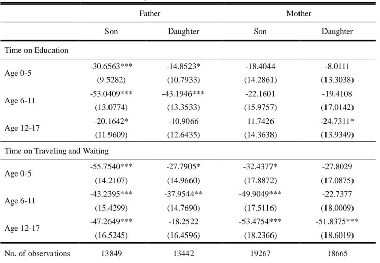
childcare time on education and traveling and waiting, the two subcategories that are most correlated with children’s human capital investment. We also find that parents with different education attainments react similarly to state industrial structure, although highly educated mothers spend less childcare time on traveling and waiting if they live in states with many labor-intensive jobs. Finally, we find that the effect of state industrial structure on parent’s time spent on children’s education mainly occur among parents with children aged 11 or less, while the effect on childcare time spent on traveling and waiting is pervasive among parents with children of all ages. This final result suggests that state industrial structure may affect the human capital investment in children very early on.

The remainder of this paper is organized as follows. After the Introduction, in section 2 we will provide a brief literature review. Section 3 describes the data as well as our construction of variables. Section 4 illustrates our empirical specifications and reports our results, and Section 5 concludes the paper.

II. Literature Review

Previous literature mainly focuses on the correlations between childcare time and family structure or parental characteristics. Bianchi (2000, 2010) study multiple US historic time use surveys and conclude that married mother spend more parental childcare time than single mothers, although single mothers still average 83 to 90 percent as much time with their children as married mothers. Kimmel and Connelly (2007) study the 2003 and 2004 American Time Use Survey and find that childcare time increases with the number of children, decreases with the age of the child, and increases with the price of child care; Price (2007) documents the relationship between birth order, birth spacing, and parental time, and he argues that the parents’ apparent desire for equity at each point in time actually leads to inequities in the total time resources received by each child.

4

Parental time investment in children has also been found to be positively correlated with parents’ education attainments. Based on data from thirteen countries, Guryan, Hurst, and Kearney (2008) find that despite the longer working hours, high education parents still spend more childcare time than low education parents.3 , 4 Gimenez-Nadal and Molina (2013) estimate a seemingly unrelated regression (SUR) model to take into account that the time one parent devotes to childcare activities may serve as a substitute for the time devoted by the other. They find that in Spain and UK it is the mothers’ education level that matters for parental childcare time, while that of fathers’ are less important. Many studies focus on how parents’, especially the mothers’, labor market participation, affect parental childcare time. For example, both Kimmel and Connelly (2007) and Bianchi (2010) find that women in the United States who participate in the labor market spend less time with their children, although Sayer et al. (2004) argue that parents who have school-age children do not spend less time as children’s school hours coincide with parents’ work hours.5

Relatively few studies explicitly focus on how societal changes affect parental time investment in children. One notable exception is Ramsey and Ramsey (2010), who use multiple time use survey data between 1965and 2007 and find that since 1990 American parents have significantly increase their childcare time, with most of the increase coming In terms of time trends, Bianchi (2010) documents an increasing trend in parental childcare time, so despite a much higher labor market participation rate, by 2000 the employed mother was recording as much primary childcare as the nonemployed mother recorded in 1975. This is made possible as today’s mothers financed their childcare time with less leisure and housework.

3 _{They studied 14 countries, including the United States, Australia, Canada, Chile, Estonia, Italy, France,}

Germany, Netherlands, Norway, Palestine, Slovenia, South Africa, and the United Kingdom.

4

They argue that this result could arise if child care is more of a luxury good than other consumption

commodities; if higher-educated parents have a lower elasticity of substitution between own and market-based child care or just a higher relative preference for time spent with their children; or if the returns to investing in the children of higher-educated parents are higher than the returns to investing in the children of lower-educated parents.

5

from time spent on education and traveling. They argue that this occurs because of increased competition for college admissions, and they provide empirical support with a comparison of trends between the United States and Canada, across ethnic groups in the United States, and across U.S. states. They further compare the increase among high education and low education parents, and find the increase is more pronounced among high education parents. They postulate that college-educated parents have a comparative advantage in preparing their children for college, so when competition for admission rises, these parents have the most incentives to drive the college preparation upward.

Similarly to Ramsey and Ramsey (2010), this paper attempts to link parents’ childcare time to difference in social environment, though the explanation provided here is the difference in industrial structures across states. We argue that the difference in industrial structure will give rise to different payoffs of education, and this will result in different incentives in time investment in children.

III. Data Descriptions

The main data used in this paper comes from the 2003-2010 American Time Use Survey (ATUS). The participants in ATUS, which include individuals over the age of 15, are drawn from the existing sample of the CPS, and they are surveyed approximately 3 months after completion of the final month of the CPS survey.6 The ATUS asks the participants to recall the activities done in the previous day, so it allows one to measure the amount of time people spend doing various activities, such as paid work, childcare, socializing, etc.7

6 _{The number of household sampled in the ATUS is around 13000 each year, though in 2003 there are around}

20000 households in the sample.

It also ask questions about the specific person(s) around when doing each activity, so in our case, we can infer which child the parents are taking care of in each childcare-related activity.

6

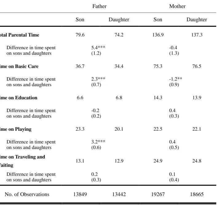
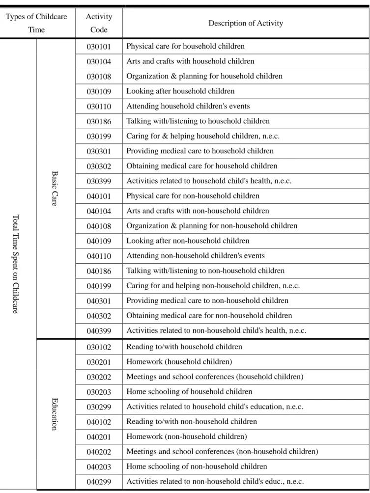
In this paper, we follow Guryan, Hurst, and Kearney (2008) and define children to be family members below 18. We consider four types of childcare time: basic care, education, playing, and traveling and waiting, and the total time spent on these four types of activities constitute the total childcare time. Descriptions of the childcare activities covered are detailed in table A1 in the appendix.

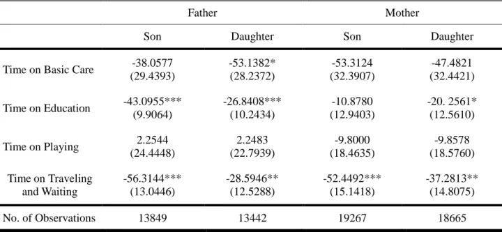
Table 1 summarizes the time spent on each son or daughter among parents. Here, our sample only includes parents who have at least one child aged 18 or less within the household. As we can see from table 1, mothers on average spend much more time (around 137 minutes per day) on childcare then fathers (around 75 minutes per day), and the amount of time they spent on basic care, education, and traveling and waiting basically doubles that of fathers. The sole exception is time on playing, where we see little difference between mothers and fathers. Table 1 also gives information on the time parents spent on children of different genders. As we can see, in total fathers significantly spend more time on sons than daughters, where the difference arises from time on basic care and playing. However, mothers’ childcare time does not seem to differ among sons and daughters.

Table 2 further summarizes childcare time among parents of different education attainments. Here, as in previous studies such as Guryan, Hurst, and Kearney (2008) and Ramsey and Ramsey (2010) we find a positive relationship between parents’ education attainments and childcare time, and this positive relationship holds among both mothers and fathers, and also among all four types of childcare activities. Again, we find that, except for time on playing, mothers’ childcare time doubles fathers’ childcare time.

As this paper is to study the relationship between a state’s industrial structure and parental childcare time, we combine employment information from the 2000 Census and the occupational characteristics from the occupational information network (O*NET) to calculate

7

the share of labor intensive jobs in each state.8

The O*NET provide information on the importance and the requirement of different abilities in each occupation, and here we specifically focus on the physical abilities required in occupations.

As described earlier in the introduction, we focus on labor intensive jobs because these jobs are more “localized” in the sense that they are usually held by local low skilled incumbent residents, who have been found in the literature to have a much smaller migration rate. Therefore, we hypothesize that parents living in states with more labor intensive jobs are less adamant about their children’s education outcomes because they know that even if their children do not do well in school, they still can easily find local labor-intensive jobs.

9

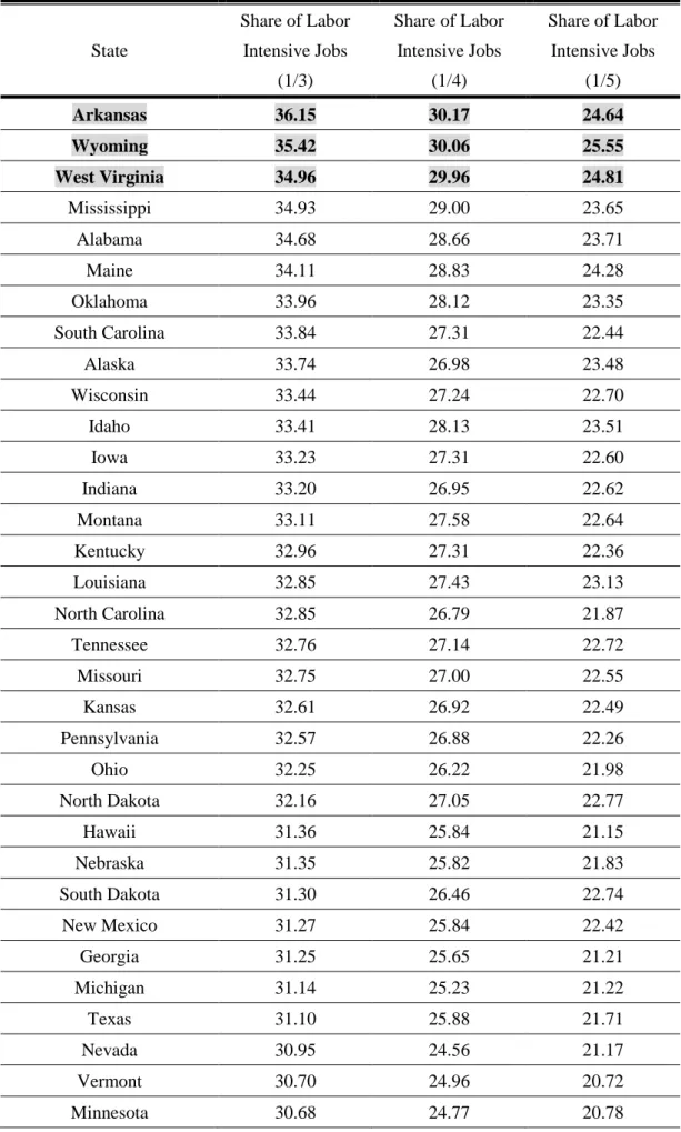
From the first column in table 3, we find large difference in industry structure across states. Specifically, we find the three states (Arkansas, Wyoming, and West Virginia) with the largest share of labor intensive jobs have over 35% of their jobs been classified as labor intensive, while the three states (District of Columbia, Maryland, and New Jersey) with the smallest share of labor intensive jobs only have around 25% of their jobs been classified as labor intensive. In the second and third columns in table 3, we generally find that the ordering of states in terms of its industry structure does not change when we redefine labor intensive jobs as those occupations with top 1/4 or 1/5 scores in physical requirement. Hence, in our empirical study we simply focus on the result where labor-intensive jobs are defined as occupations with top 1/3 physical requirement scores.

As the O*NET identifies 9 types of physical abilities and give scores on each of them, we take the simple average of the scores to represent the physical requirement for each occupation. Based on these scores, we identify the occupations with the top 1/3 scores and label them as labor-intensive jobs. We then calculate the share of labor intensive jobs in each state and the results are given in table 3.

8 _{Census Information is obtained from the Integrated Public Use Micro data Series (IPUMS). The O*NET}

information is obtained directly from its website: www.onetonline.org.

8

IV. Empirical Specifications and Results

Empirical Specification

In order to investigate how the share of labor-intensive jobs within a state affects parents’ childcare time, we consider the following regression model for individual i living in state j at year t:

ParentalTime_ijt = αX_i+ βLaborJobs_j+ Time_t+ ε_ij (1)

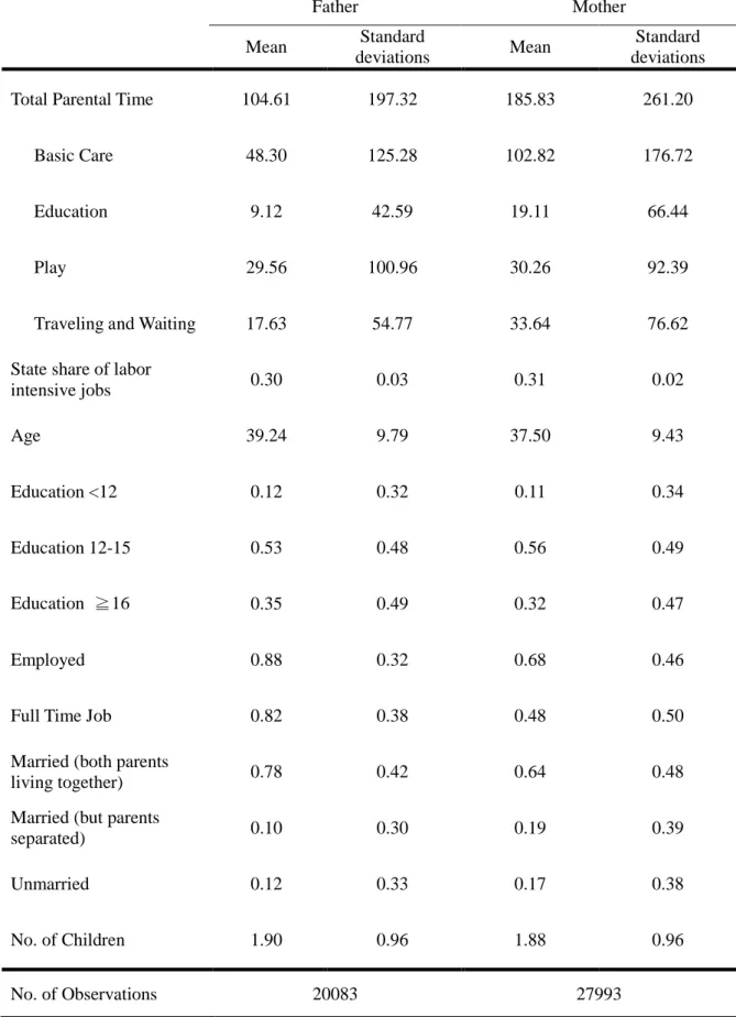
Here, ParentalTime_ijt denotes the parental childcare time, where in our empirical implementation we will consider total childcare time as well as each subcategory of childcare time. LaborJobs_j is our main variable of interest, and it denotes the share of labor intensive jobs within the state the household resides. X_i represents a series of individual characteristics, such as age, parent’s education level, parent’s employment status, marital status, and the number of children within the household. These additional controls are often used in this strand of literature. Finally, we add time dummies, Time_t, to control for potentially different macroeconomic conditions across survey years. The summary statistics for each variables used in the regression model is given in table 4.

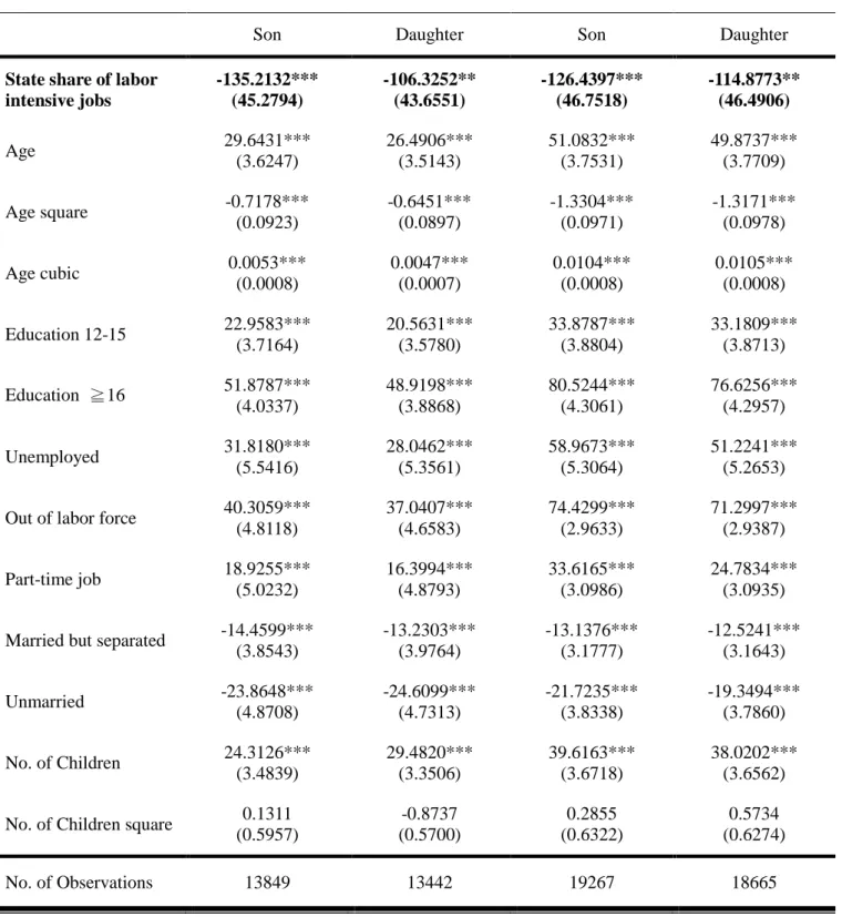
Empirical Results

The regression result for equation (1) is given in table 5. As we can see, a state’s share of labor intensive jobs is negatively correlated with parent’s total childcare time. This result holds for both fathers and mothers, and also for both sons and daughters. We argue this result occurs because parents living in states with more labor intensive jobs are less concerned about the need to get very advanced education and go into top schools as their children could still find local jobs relatively easily without a very good degree. As for the other variables, our

9

result is generally consistent with existing literature. For example, as in Guryan, Hurst, and Kearney (2008) and Ramsey and Ramsey (2010) we find childcare time increases with parents’ education attainments; parents who participate less in the labor market, either out of labor force, unemployed, or working part-time, spend more time with their children; finally, as in Kimmel and Connelly (2007), parents who have more children spend more childcare time.

We argue that the negative correlation between a state’s share of labor-intensive jobs and childcare time arises because parents are less concerned about their children’s education attainment. To verify this, we compare how a state’s share of labor-intensive jobs affects each subcategory of childcare time, and the results are given in table 6. Note here that since the time spent on these four subcategories may be correlated as they sum up to total childcare time, we use a seeming unrelated regression model (SUR) to estimate the coefficients. As we can see from table 6, although parents usually spend less time on every subcategories of childcare time, the subcategories in which there are significant differences are time on education and time on traveling and waiting: for fathers, they spend significantly less time on children in both of these subcategories, while for mothers they spend significantly less time on traveling and waiting.10

One might be concerned that our measure for the share of labor-intensive jobs may be inappropriate, so in table 7 we consider our alternative definitions of labor-intensive jobs. We find that our conclusions stated above do not change when we redefine labor intensive jobs as those occupations with top 1/4 or 1/5 scores in physical requirement.

Interestingly, these two subcategories are the ones identified by Ramsey and Ramsey (2010) and Levey (2009) to be most correlated with human capital investment in children, so the results in table 6 seem to provide some support for our hypothesis.