改善EWOD 元件於產生奈升級液滴之研究

(1)

國立交通大學

機械工程學系

碩士論文

改善 EWOD 元件於產生奈升級液滴之研究

Development of Creating Nano-Liter

Droplets using Novel Patterns of EWOD

研究生：許耀文

指導教授：陳俊勳教授

(2)

改善 EWOD 元件於產生奈升級液滴之研究

Development of creating nano-liter droplets using novel patterns of EWOD

研究生：

許耀文

Student：Yao-Wen Hsu 指導教授：陳俊勳 Advisor：Chiun-Hsun Chen 國立交通大學機械工程學系碩士論文 A Thesis

Submitted to Department of Mechanical Engineering College of Engineering

National Chiao Tung University In Partial Fulfiillment of the Requirements

For the Degree of Master of Science In Mechanical Engineering

June 2007

Hsinchu, Taiwan, Republic of China

(3)

摘要

電濕潤是藉由氣液介面的表面張力影響來液珠，而使液珠移動，其中優點包含，製造過程簡單、可控制定量的液珠、價格較低可取代微制動器與微混合器等。本研究先簡化質量守恆方程式與動來守恒方程式來當作電濕潤的模擬模式，並利用商用軟體 CFD-ACE+來模擬液珠在電濕潤的情況。而電濕潤元件的組成包含，8 個 0.48mm X 0.5mm 的底部電極（金 /鉻）、介電層厚度為 3000Å 的氮化矽、厚度為 1000 Å 的鐵福龍層和旋塗厚度 1000 Å 鐵福龍的氧化銦錫玻璃為上電極。其實驗量測系統包含，微流體元件、微處理器、控制電路、LCD 顯示器、4X4 小鍵盤、電源供應器和功率放大器。幾種不同設計的電極形狀會先在模擬情況下互相比較，總共有 16 組，將常用的正方形電極改成指插電極，並改變流道高度 (20μm 、35μm和 70μm)、指插電極角的數目與指插電極角的寬度，來探討液珠的壓力與平均速度之變化，其中，液珠的內壓與大氣壓的壓差會隨著流道高度的縮小而變大的情形亦被模擬，也於流道高度為 35μm的模改善 EWOD 元件於產生奈升級液滴之研究學生 : 許耀文指導教授 : 陳俊勳國立交通大學機械工程學系

(4)

奈升液珠，以便於在生醫上的應用。最後根據模擬的預測，選取 3 種的電極設計，並利用微機電技術製造元件來證明模擬的趨勢，其中選取的電極分別為正方形電極，指插電極角數目為 2323 的排列與 5656 的排列順序。對於液珠在流道高度為 20μm的移動情況下分別作平均速度的比對，其中，在實驗上液珠的平均速度對於排列順序為 2323 的指插電極為 11.36 mm/s，而模擬的平均速度為 13.291 mm/s。對於電極排列順序為 5656 在實驗與模擬的平均速度分別為 11.07 mm/s 和 11.542 mm/s。而正方形分別為 10.49 mm/s 和 9.614 mm/s。最後，在實驗上於應用電壓為 100V 的交流電下，也成功產生出 2.9～8.5nl 的奈升液珠。關鍵字：電濕潤，指插電極，CFD-ACE+

(5)

ABSTRACT

Electrowetting on dielectric (EWOD) moving fluid driven by surface tension offers some advantages, including simplicity of fabrication, control of minute volumes, low cost, substitution for micro-mixers and others. In this study, The EWOD model based on the reduced forms of the mass and momentum conservation equations is adopted to simulate the fluid dynamics of droplet, and its movement is simulated by a commercial software CFD-ACE+. The EWOD device consists of eight 0.5 x 0.48 mm bottom electrodes (Au/Cr), a dielectric layer of 3000 Å nitride, a Teflon layer of 1000 Å and a piece of indium tin oxide (ITO)-coated glass with 1000 Å Teflon as the top electrode. The measurement system consists of the microfluidic device, microprocessor, electric circuits, LCD module, keypad, power supply and power amplifier. Several simulations using different electrode designs were carried out in advance. The interdigitated electrodes were used to replace

Development of creating nano-liter droplets using novel patterns of EWOD

Student: Yao-Wen Hsu Advisor: Prof. Chiun-Hsun Chen Institute of Mechanical Engineering

(6)

electrodes. Sixteen simulations were carried out in this thesis. Under the same shape of interdigitated electrode, the phenomenon of increasing pressure difference due to decrease of channel height can be simulated. For simulations of 35

μ

m-channel height, the ones with interdigitated electrode can generate the larger pressure differences (310 Pa~680 Pa) than that of square electrode (300 Pa). The increment of pressure difference is helpful to move and cut droplets, and further to create a nano-liter droplet, which can be applied in biomedical applications. The following optimal designs of electrode were according to the best simulation results. Then, they were manufactured by MEMS processes and their performances were certified by EWOD device. Furthermore, the predictions of simulations for droplet of moving, in which the channel height was 20μm were compared with experimental results for three designs of electrodes including square electrodes and interdigitated electrodes with arrangements of 2323 and 5656 extended rectangles. It is found that the mean velocity of droplet for interdigitated electrode (2323) was 11.36 mm/s, whereas the corresponding prediction was 13.291 mm/s. For 5656 arrangement, the mean experimental and numerical velocities were 11.07 and 11.542 mm/s, respectively. As to square electrode, they were 10.49 and 9.614 mm/s, separately. Finally, the 2.9nl~8.5nl droplets are successfully created at 100 VAc experimentally.

Keyword: CFD-ACE+, Electrowetting on dielectric (EWOD), interdigitated electrode

(7)

ACKNOWLEDGEMENT

回看兩年碩士生活自覺得有許多成長，其中最感謝陳俊勳老師，讓我有機會在成大電機系張凌昇老師的研究室學習不同的領域，並能在求學期間將所遇到的問題能一一克服，對於未來競爭力上學生覺得受益良多，在此對兩位老師獻上無限的感激與敬意。其中在研究過程中，要特別感謝交大的文耀、國華、關恕、嘉鴻、靜慈、遠達、彥成、等學長姐在碩班生活上的指導，還有、迪翰、建宏、炳坤、等同學的幫忙與鼓勵。而在成大生涯中也特別感謝宜良、垣杰、敏峰、智淵、偉雄、浩凱、浩君、俊宏、信宏、俊慶、威宇、南江、鎵豪等人在台南的幫忙，讓我在成大做研究及生活上更加得心應手。當然也要特別感謝我的好朋友振華在成大的照顧。最後感謝我的家人在我求學過程中的一路陪伴與鼓勵，謝謝。

(8)

LIST OF TABLES

Table 3-1 Electrode shapes... 39

Table 4-1 Volume of droplet... 54

Table 4-2 Simulation properties ... 55

Table 4-3 16 cases of droplet moving simulations... 57

Table 4-4 Pressure difference vs. channel height... 62

Table 4-5 Pressure difference vs. the same contact curve (area) ... 64

Table 4-6 16 cases of cutting... 65

Table 4-7 the hydrolysis energy ... 69

(11)

LIST OF FIRGURES

Fig. 1-1 Scaling of weight and surface tension [3] ... 8

Fig. 1-2 Move liquid metal (mercury) in the electrolyte by CEW [5] . 8 Fig. 1-3 Illustration of continuous electrowetting device [6] ... 9

Fig. 1-4 Illustration of method to move droplet by EWOD [7] ... 9

Fig. 1-5 Contact angle and its surface tension [7]... 9

Fig. 1-6 The field applied changes the surface tension at the liquid-solid and liquid-vapor interfaces, causing the droplet to flatten [7] ... 10

Fig. 1-7 Digital and addressable microfludic circuit [9]... 10

Fig. 1-8 Contact angle of droplet changed in the parallel plates [5].. 11

Fig. 1-9 Separation of two types of particle [10] ... 11

Fig. 1-10 Control particle concentration [10] ... 12

Fig. 1-11 The optical detection instrumentation [11]... 12

Fig. 1-12 The trinder reaction of glucose concentration [11] ... 13

Fig. 1-13 Creating nano-liter by auto-control system [12] ... 13

Fig. 1-14 The relative illustration of channel height and manipulative frequencies [13]... 14

Fig. 1-15 Comparison between simulation and experiment [14][15] 15 Fig. 2-1 Illustration of Electrical Double Layer [2] ... 31

Fig. 2-2 Surface tension changed by Electrical Double Layer [2]... 31

Fig. 2-3 Illustration of basic model used to deduce equations [14] ... 32

Fig. 2-4 Equivalent circuit of EWOD in the parallel plates [1] ... 32

Fig. 2-5 Illustration of deducing pressure difference ... 33

Fig. 2-6 Illustration of droplet moved by different pressure... 33

Fig. 2-7 Views of X, Y and Z directions of droplet cutting [9]... 34

Fig. 2-8 Schematic diagram of free surface reconstructions: (a) actual interface; (b) SLIC approximation; (c) PLIC approximation .... 35

Fig. 2-9 SIMPLEC algorithms ... 36

Fig. 2-10 Evolution of the pressure difference against grid density (case 05) ... 37

(12)

pattern of pictures of EWOD control electrodes... 49

Fig. 3-6 Illustration of EWOD process ... 51

Fig. 3-7 Illustration of top plate process ... 52

Fig. 3-8 The SEM photo of EWOD device... 52

Fig. 3-9 Measurement of contact angle... 53

Fig. 4-1 Illustration of Table 4-3 ... 71

Fig. 4-2 Illustration of velocity and pressure for droplet (case 1) ... 72

Fig. 4-3 Pressure and velocity vs. time for case 1 (triangle: pressure of head droplet; square: pressure of tail droplet; circle: velocity of droplet head; diamond: velocity of tail droplet)... 73

Fig. 4-4 Illustration of velocity and pressure for droplet (case 3) ... 74

Fig. 4-5 Pressure and velocity vs. time for case 3 (triangle: pressure of head droplet; square: pressure of tail droplet; circle: velocity of droplet head; diamond: velocity of tail droplet)... 75

Fig. 4-6 Simulations of moving (channel height 35μm)... 77

Fig. 4-7 The contact length of droplet occupying adjacent electrode 78 Fig. 4-8 Situation of moving droplet touching the adjacent electrode ... 79

Fig. 4-9 The contact length of droplet to next electrode for coae-05, 08 and 10 (Table 4-2) ... 80

Fig. 4-10 Using tension to illustrate contact curve into adjacent electrode ... 80

Fig. 4-11 Pressure difference increases with area of electrode ... 81

Fig. 4-12 Simulations of cutting (continue with Fig. 4-2) ... 83

Fig. 4-13 Simulations of cutting for droplet beginning position in middle electrode (channel hright 70μm) ... 84

Fig. 4-14 Simulations of cutting for droplet moving from left to middle electrode (channel hright 70μm) ... 85

Fig. 4-15 Comparison of cutting for interdigitated electrode and square electrode at channel height 70μm ... 86

Fig. 4-16 Pressure distribution of interdigitated electrode (232) at channel height 70μm... 87

Fig. 4-17 Photos of creating (interdigitated electrode 2323) ... 88

Fig. 4-20 Photos of creating (square electrode) ... 91

Fig. 4-21 square electrodes... 92

(13)

Fig. 4-23 the total capacitor of interdigitated electrodes ... 93 Fig. 4-24 Comparison between simulation flames and experimental

photos (interdigitated electrode 2323, channel height 20μm) ... 94 Fig. 4-25 Comparison between simulation flames and experimental

photos (interdigitated electrode 5656) ... 95 Fig. 4-26 Comparison between simulation flames and experimental

(14)

NOMENCLATURE

0

γ

Surface tension of solid-liquid interface without external potential

γ

_{Surface tension of solid-liquid interface with external potential}

c Capacitance per unit area

R

Radius of ideal sphere of droplet

V Potential

sys

E _{Total energy of the system}

int

E Interfacial potential energy of the droplet

de

E Energy stored in the solid dielectric layer between the liquid and the counter electrode

vs

E Potential energy

SL

γ

Interfacial tension between the solid-liquid

SV

γ _{Interfacial tension between the solid-vapor}

LV

γ Interfacial tension between the liquid-vapor

SL

A _{Area of the droplet on the solid surface}

LV

A _{Liquid-vapor interface area}

v

Volume of the dielectric layer

Er Electric field

Dr Charge displacement

0

ε

permittivity of vacuum

r

(15)

d Dielectrics of thickness

0

θ

Contact angle without external voltage

θ

Contact angle with external voltage C Capacitance

Q Charges in the capacitor.

Top

C _{Capacitor on the top plate}

Botton

C _{Capacitor on the bottom plate}

p

Δ

Pressure difference across an interface

a

P

Pressure of atmosphere D Distance of channel gap

1

R Radius of curvature of the droplet curved surface

x X direction y _{Y direction} z Z direction Vv Velocity vector p _Pressure ρ _{Fluid density}

μ

_{Viscosity coefficient} σ

(16)

σ Surface tension value

ˆ

(17)

CHAPTER 1 INTRODUCTION

1.1 Motivation and background

As micro-electro-mechanical-systems (MEMS) technology requirement increases, microfluidics has become possible to be controlled. In the last several decades, there has been a tremendous of interests in the movement of bulk fluidic mass and in the path control of the embedded objects of interest (e.g., cell, protein, etc.) in the flow. The so-called biochips, which integrate microfluidic and microsensor devices, have potential application in chemical analysis, drug delivery, protein analysis, gene expression, biochemical analysis, detection, and so on [1]. Traditionally, chemical analyses have been performed in central laboratories by skilled personnel and specialized equipments. However, the trend is to push chemical analyses closer to ”customer.” To let it come true, handy and portable analytical equipments, such as biochips, are needed [2]. The major advantages of biochip are that it can minimize reagent consumption, reduce analysis time, increase sensitivity and improve accuracy. Therefore, biochip is currently one of the microsystem engineering fields with the largest market opportunities.

The developed biochips basically can be divided into two categories; one is the microarray chip and the other the lab-on-a-chip. Microarray chip has ripened into maturity, on the other hand, lab-on-a-chip is becoming the potential research topic in the near future. Lab-on-a-chip－well-known as

(18)

laboratory by a chip. It can push liquid in the order of microlilter or nanolilter into a chip, which is covered with micro fluidic channels fabricated by the semiconductor processing technology, and then there is the same response of liquid in the designed chip as required in lab.

During the last several decades, many microsystems have been investigated and developed to control liquid movement under the microscale. In those microfluidic systems, there exist many methods, such as electrowetting, electrostatics, electrophoretics, electroosmotics and thermopneumatics, to drive liquid. The traditional one has been using microfluidic channel to control continuous-flow. Until very recently, the actuation based on surface tension becomes a dominant mechanism on the microscale device. Fig. 1-1 illustrates the scaling of two forces for weight and surface tension, respectively [3]. The effect of surface tension is greater than that of weight when the system dimension is below the sub-microscale. Actuation of the droplet based on the change in surface tension can eliminate the need for moving parts and can be performed by programmed electric signals rather than physical structures. Droplet-based microfluidic systems differ from continuous flow ones because they manipulate discrete droplets rather than continuous flow. The electrical control of wettability of liquids on a dielectric material, called electrowetting- on-dielectric (EWOD), has drawn much attention as a promising microfluidic actuation mechanism in micro total analysis systems (μTAS). EWOD has an excellent reversibility and it possesses a number of advantages over continuous-flow systems, such as controlling each droplet independently, minimizing the usage of fluids, reducing the mixing time and having the comparable performance with the traditional methods. Due to the advantages mentioned above, EWOD technology has a great potential industrial market in the future.

(19)

1.2 Literature review

The mechanism of EWOD is that when an electric voltage is applied to the droplet, the electric charge changes free energy on the dielectric surface, inducing a change in wettability of the surface and resulting in the change in the droplet contact angle. The concept of electrowetting (EW) originates from the Lippman, who made an experiment about electrocapillarity in 1875 [4]. He recognized that the externally added electrostatic charge can change the capillary forces at an interface. Fair et al. [5] firstly proposed that using EW changes the liquid-to-liquid surface tension to move liquid metal (electrolyte) in the mercury and solution in silicon oil (Fig.1-2-a). Kim [5] was successfully to drive the solution in air by changing liquid-solid surface tension, as shown in Fig.1-2-b.

The continuous electrowetting (CEW) was developed by Fair et al. [5-6]. The electrowetting microactuator is presented schematically in Fig.1-3. A droplet of polarization and conductive liquid was sandwiched between two sets of planar electrodes. The upper plate consisted of a single continuous ground electrode, while the bottom one consisted of an array of independently addressable control electrodes. The control electrodes were then coated with 7000 Å of Parylene C followed by approximately 2000 Å of Teflon AF 1600. Both electrode surfaces were covered by a thin layer of hydrophobic insulation. Droplets of 100 mM KCl solution were successfully transferred between these two electrodes at the voltages of 40–80 V. Repeatable

(20)

surface tension, a main driving force. As shown in Fig.1-4 [7], by turning electrodes on and off in prescribed sequences, it was possible to induce droplets to move to specific locations. By switching on the voltage at an electrode adjacent to the droplet, the surface tension was lowered locally, causing the droplet to move to the right. It returned to its original shape when the potential was switched off. The change of contact angle could be obtained from surface tension. It is easier to drive droplet, because the more contact angle changes, the more surface tension changes. Figures 1-5 and 1-6 illustrate that the contact angle of droplet is changed by the external voltage [7].

The contact angle decreases as the applied potential increases until the contact angle is saturated, and then it is called contact angle saturation, which the angle can no longer increase even by applying higher voltage. In order to understand the phenomenon of contact angle and contact angle saturation on the different material with different samples, it is completely relied on the design and control of microfluidic system. The reason of saturation at DC voltage and AC voltage are not exactly the same. For the AC signal, it creates ionization between sharp-pointed area of droplet and air, and then the droplet is surrounded by ions in a form of a hydrophilic ring, which can destroy the hydrophobia of dielectric layer. For the DC signal, the charges are trapped in the dielectric layer, after that they form the hydrophilic ring to destroy the hydrophobia of dielectric layer and make the electrowetting irreversible [8]. The electrowetting irreversibility can be improved by suitable dielectric material. Besides saturated phenomenon, it has a little difference to the change of contact angle as increasing and decreasing voltage, which is called hysteresis. These shortcomings can be improved better by applying suitable dielectric material and MEMS process.

(21)

In the microfluidic system, the control of digital microfluidics comprises four basic operations: (a) creating, (b) transporting, (c) merging and (d) cutting liquid droplets. The pioneer study was done by Kim et al. [9]. In addition to the four operations mentioned above, they designed the NxM grids, as shown in Figs.1-7 and 1-8, that various kinds of products can be produced in the NxM channels by the reservoir of X-direction and Y-direction.

It is often to see an experiment about the concentration control and the separation of cells, molecules and particles. Kim et al. [10] accomplished to separate two types of particle by property of electrophoresis and EWOD control, as shown in Fig. 1-9. The procedure consisted of four steps. The first one, a droplet containing mixed particles was placed between two parallel plates (Fig.1-9-a). The second one, separated (isolate) particles by electrophoresis within a droplet (Fig.1-9-b). An electric field was applied between two exposed electrodes on the top plate to isolate one type of particles on the left side and the other on the right side. The third one, cut the droplet by EWOD actuation after the particles were separated (Fig.1-9-c). The detailed design rules, mechanisms and experimental verifications for the cutting process of droplets were reported. A smaller channel height, a larger droplet size and a larger change in the contact angle enhance the necking of the droplet to help the completion of the cutting process. The last one, transported the produced droplets by EWOD to other locations for the next microfluidic operation (Fig. 1-9-d). To improve the precision of separation, multiple droplets with the same particle type can be re-joined and may go through further separation in the next stage. If there is only single type of

(22)

It was judged the percentage of glucose concentration with the changes of reagent colors detected by optics instrument, as illustrated in Figs.1-11 and 1-12. They found that the measurement of glucose concentration can be finished in less than one minute.

H.Ren et al. [12] was successful in producing droplet of nano-liter in silicon oil by using auto-control system and AC voltage, as shown in Fig.1-13.

Chatterjee et al. [13] firstly reported that organic solvents, aqueous surfactants and ionic liquids can be manipulated in air in EWOD. The method of actuation is to input AC with various frequencies to drive different liquids, as shown in Fig.1-14.

From the literatures given above, techniques for digital microfluidic devices tend to be mature, after that, it can be applied to bio-samples delivery and cell analyses in the near future. Of course, it is expected to reduce the amount of samples used, analyzing time and prime cost.

1.3 Scope of this study

In this laboratory, a method was developed to simulate EWOD phenomenon. The pictures obtained from the simulation were compared to experimental photos, as shown in Fig. 1-15, in which the applied voltage was 40V, dielectric thickness (nitride) 3000Αo , channel height 70 mμ , length of electrode 2mm and volume of droplet 0.3 lμ . It can be seen that the results of simulation and experiment agree well, indicating that all of the simulation parameters are verified, and these can be used to simulate and design the new electrodes [14, 15].

The purpose of this study is to generate a nano-liter droplet by EWOD device. The micro-liter for a volume of cell is still too big if it wants to catch

(23)

cells and to analyze them. For cells in micro-liter liquid, the concentration of liquid (extracellular space) will be changed by its metabolism, however, the changed concentration is not obvious in micro-liter. If want to measure the concentration of liquid, it needs a high sensitive instrument. However, if the volume of droplet can be as small as possible, then, the changed concentration can be measured easily. Due to this reason, it needs to limit the range of cell movement and to be able to create nano-liter droplet. In this thesis, a commercial software CFD-ACE+ is adopted to simulate how to create a nano-liter droplet and then fabricate the corresponding device to prove it. It also will discuss the relationship between the shapes of electrode and EWOD driving forces.

(24)

Fig. 1-1 Scaling of weight and surface tension [3]

(25)

Fig. 1-3 Illustration of continuous electrowetting device [6]

(26)

Fig. 1-6 The field applied changes the surface tension at the liquid-solid and liquid-vapor interfaces, causing the droplet to flatten [7]

(27)

(28)

Fig. 1-10 Control particle concentration [10]

(29)

Fig. 1-12 The trinder reaction of glucose concentration [11]

(30)

Fig. 1-14 The relative illustration of channel height and manipulative frequencies [13]

(31)

Fig. 1-15 Comparison between simulation and experiment [14][15] t=0~0.033 t=0.066~0.099 t=0.132~0.165 t=0.198~0.231 t=0.264~0.33 t=0~0.033 t=0.066~0.099 t=0.132~0.165 t=0.198~0.231 t=0.264~0.33

(32)

CHAPTER 2 MATHEMATICAL MODEL AND NUMEICAL

METHOD

2.1 Mathematical method

The actuation principle of EWOD is that a droplet is placed on an electrode covered first by a dielectric layer and then Teflon layer. Because the hydrophobic stuff makes contact area of liquid and solid decreasing, the droplet contact angle is larger than the one without coating of dielectric layer [1]. When the potential is applied, the altered stored electric charge density in the liquid-solid interface makes droplet contact angle becoming smaller. The main driving force is surface tension. It causes droplet contact angle to change after the potential is applied on adjacent electrodes, and the droplet is driven by the different pressure between the inside and outside of the droplet. The surface tension magnitude is obtained by the change of droplet contact angle. The knowledge of the contact angle and its corresponding saturation for different liquids on different materials can be used to design and control the microfluidic devices. The equations for EWOD are as follow:

2.1.1 Electric double layer

While liquid metal, as mercury, is immersed in electrolyte, the interface between two media becomes electrically charged owing to various electrochemical activities to cause adsorption of electrolyte ions on metal surface. This interface is named polarizable interface, electrified or electric double layer (EDL) [2]. The EDL thickness is around 10-100Ao depending

(33)

on the kind of electrolyte-metal pair, concentration of the electrolyte, electrical condition and temperature. In Fig. 2-1, the charged density is originally distributed uniformly along the X-direction while no external potential. The liquid-metal containing the EDL is positive charged and the electrolyte is negative charged. If a potential is applied between the two electrodes in the electrolyte, a low current flows across the electrolyte between the liquid metal and the channel wall resulting in a decrease in voltage along the X-direction, as shown in Fig.2-2 [2]. The potential difference across the EDL produces a surface tension gradient to move liquid metal from left to right. It has been found that a thin dielectric layer inserted between the electrode and droplet can emulate in EWOD.

2.1.2 Lippman’s equation

In 1875, Lippman made an electrocapillarity experiment, and found firstly that the capillarity force is changed by external electric charges on the interface between liquid metal and electrolyte. The Lippman’s equation for the capillarity phenomenon is as follow:

2 0

1

2 cV

γ γ

=

−

_{, (2.1)}

where γ0 is the surface tension of solid-liquid interface without external

potential (V =0), c the capacitance per unit area of EDL and V the applied voltage. In EWOD phenomenon, Lippman equation mainly discusses the relationship between external voltage and surface tension.

(34)

radius

R

and the contact angle

θ

(see Fig. 2-3). Moreover, the system is in equilibrium at constant potential V . Any effects of the droplet edge like stray capacitance are neglected. The contact angle hysteresis for increasing and decreasing voltage is not considered and the droplet volume

v

is considered to be constant, i.e., dv = . The contact angle 0

θ

is the angle between the liquid-vapor and the solid-liquid interface at the triple phase point.

θ

varies with the applied voltage and hence the droplet shape changes. The total energy of the system,

E

sys, is expressed as [16]:

int

sys de vs

E

=

E

+

E

+

E

_,_(2.2)

where

E

int is the interfacial potential energy of the droplet,

E

de is the

energy stored in the solid dielectric layer between the liquid and the counter electrode, and

E

vs is the potential energy, performed by an external voltage

source to redistribute the charges when the shape of the droplet changes.

sys

E

is minimum at equilibrium so that the total differential of the energy,

sys

dE

, is equal zero. As the functions of

R

and

θ

,

dE

sysis given by:

( , ) ( , ) [ sys] [ sys] sys E R E R dE dR d R θ θ θ θ ∂ ∂ = + ∂ ∂ . (2.3)

Equation (2.3) expresses that at equilibrium of the system, any infinitesimal change in energy due to shape variations of the droplet must be zero. With the restriction of a constant droplet volume (dv = ), Shapiro et al. rewrites Eq. 0 (2.3) as 2 2 2 cos ( ) cot( ) ( , ) ( , ) 2 cos ₂ ₂ ( ){[ ] ( ) [ ]} 0 2 sin 2 cos sys sys E R E R R R R θ θ θ θ θ π θ θ θ ⋅ ∂ ∂ + − ⋅ ⋅ − + = ∂ + ∂ . (2.4)

It firstly considers a droplet on the dielectric layer while no external voltage is applied to the system (

E

de = 0 and

E

vs= 0). The system energy is defined

(35)

as the interfacial potential energy of the droplet (

E

int). int

(

SL SV

)

SL LV LV

E

=

γ

−

γ

⋅

A

+

γ

⋅

A

_._(2.5)

The energy of a liquid on a solid surface depends on the interfacial tension between the solid-liquid

γ

SL, the solid-vapor

γ

SV and the liquid-vapor

γ

LV

interface. The subscript L, V and S denote liquid, vapor and solid phases, respectively.

A

SL is the base area of the droplet on the solid surface and

LV

A is the liquid-vapor interface area. Both are defined by

R

and

θ

as:

2 2 ( , ) sin SL A R

θ

=

π

R

θ

. (2.6) 2 ( , ) 2 (1 cos ) LV A R

θ

=

π

R −

θ

. (2.7) Using Eqs. (2.5), (2.6) and (2.7), the system energy is expressed as

2 2

( , )

[(

)

sin

2 (1 cos )]

sys SL SV LV

E R

θ

=

R

γ

−

γ

⋅ ⋅

π

θ γ

+

⋅ ⋅ −

π

θ

. (2.8) Combine Eqs. (2.4) and (2.8), the Young equation can be derived as

cos SV SL LV γ γ θ γ − = . (2.9)

It considers the case, which an external voltage V is applied to the system. Besides, in the previous case the potential energy,

E

de , stored in the

dielectric layer between the liquid and electrode counter contributes to the total energy 0 1 ( , ) 2 de v E R

θ

=

ε

∫

EDdvr r _, _(2.10)

(36)

integrating Eq. (2.10),

E

decan be written as: 2 0

1 ( , )

2

de r SL

V

E R

A

d

θ

=

ε ε

_._(2.11) de

E

is equivalent to the energy stored in a plate capacitor filled with a

dielectrics of thickness d. The base of the droplet

A

SL defines the size of

one electrode. Any change in the droplet shape appears as a change in the capacity and requires a redistribution of the charge. The necessary work performed by the external electrical source is twice the potential energy stored in the dielectric layer. The negative sign for the electrical energy

E

vsin Eq.

(2.12) corresponds to this fact:

2 0 ( , ) de r SL V E R A d

θ

= −

ε ε

_._(2.12)

Combining Eq. (2.5), (2.11) and (2.12), the system energy is given by:

2 2 0 2

( , )

[(

)

sin

2 (1 cos )]

2

r sys SL SV LV

V

E

R

d

ε ε

θ

=

γ

−

γ

−

⋅ ⋅

π

θ γ

+

⋅

π

⋅ −

θ

_, (2.13) and together with Eq. (3), the Young-Lippman equation is recovered as:

2 0 0 1 cos cos 2 rV d ε ε θ − θ = , (2.14)

Where

θ

0 is the contact angle without an external voltage and

θ

is the one

with an external voltage. The Lippman-Young equation yields the influence on the contact angle when a potential is applied to the dielectric layer.

2.1.4 EWOD in parallel plates

(37)

understand EWOD actuation of a droplet in parallel plates, it can be equivalent to an electrical circuit model of the device as shown in Fig.2-4. When DC voltage is applied, the droplet has a relationship between voltage and capacitor in parallel, as follows:

Q

C

V

=

Top Bottoms

Q

=

Q

, , DC Top DC Bottom DC

V

=

V

+

V

_(2.15)

The voltage across the top plate,

V

_{Top DC}_, , can be expressed as

, , , , Top DC Bottom DC DC Bottom DC Top DC

C

V

C

=

+

(2.16) and the voltage across the bottom plate,

V

_{Bottom DC}_, , is:

, , , , Bottom DC Top DC DC Bottom DC Top DC

C

V

C

=

+

(2.17)

Q

_{: Charges in the capacitor.}

Top

C

_{: Capacitor on the top plate.}

Bottom

C

_{: Capacitor on the bottom plate.}

It can be known that U , the electrical energy in the capacitor, becomes larger as d becomes smaller from the equation of parallel-plate capacitor

(38)

hydrophobic layer, so that C is much higher than Top CBottom. By the theory of

electrical circuits, the voltage drop is almost on bottom plate because of

, ,

Bottom DC Top DC

V

>>

V

_{; the droplet contact angle on top plate is changed}

insignificantly while the DC potential is applied on top plate.

2.1.5 Actuation force

A droplet produces a driving force on different hydrophobic surfaces, induced by the gradient of surface tension. According to the conservation of thermodynamics, it is must obey Laplace-Young equation on the interface of droplet and surrounding air. As shown in Fig. 2-5, it can deduce the equations as:

(

)(

)

dA

= +

x dx y dy

+

−

xy xdx ydy

=

+

(

)

dw

=

γ

dA

=

γ

xdx ydy

+

dw

= Δ

pxydz

1 1 1

x dx

x

xdz

dx

R

dz

R

+

₌

_→

₌

+

2 2 2

y dx

y

ydz

dx

R

dz

R

+

₌

_→

₌

+

2 1

(

)

(

dz

)

pxydz

xdx ydy

xy

R

γ

Δ

=

+

=

+

1 2

1

1 (

)

p

R

γ

Δ =

+

_(2.18)

(39)

are the two radii of curvature of the droplet curved surface. In order for a droplet to produce the gradient of surface tension, it must have two dissimilar wettability contact surfaces. The pressure difference Δ is the droplet at p1

the interface between the strong hydrophobic surface and surrounding air and

2

p

Δ is the droplet at the interface of the weak hydrophobic surface and surrounding air. Because of Δ > Δp1 p2 , the droplet has a net pressure

difference that can drive the droplet, consequently, the droplet automatically moves from the strong to weak hydrophobic surfaces.

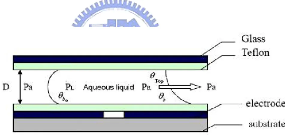
Fig. 2-6 shows that a droplet is placed between two parallel plates with a channel height h. The contact angle on the top plate is cos

θ

Top and the

bottom one is

cos

θ

Bottom. When DC voltage is applied on the right electrode,

the surface tension (

γ

sl) and θb on the right electrode are changed slightly

and then the net difference pressure drives the droplet to move toward direction with less contact angle. The pressure difference at the left droplet can be expressed as [17]: 0

(cos

cos

)

LG L a T b

P

D

γ

_θ

Δ =

−

+

_{, (2.19)}

and the pressure difference at the right droplet is

(cos

cos

)

LG R a T b

P

D

γ

_θ

Δ =

−

+

_{. (2.20)}

Combining Eqs. (2.19 ) and (2.20), the net pressure difference is:

0 (cos cos ) LG L R b b P P P D

γ

_θ

Δ = Δ − Δ = − _{. (2.21)}

(40)

From Eq. (2.22), it can be seen that the pressure difference is influenced by the channel height, dielectric coefficient and applied potential, in addition to the change of contact angle. In a controllable system, the droplet is easier to drive as ΔP becomes larger.

2.1.6 Droplet cutting

Initially, a droplet occupies the entire middle electrode as well as the portions of left and right electrodes. When DC voltage is applied at the ends but not middle, it results in making the two ends wetting and keeping the middle non-wetting. A pressure difference in the droplet drives the droplet to move toward both the left and right electrodes and causes necking in the middle electrode. This situation makes the radius of droplet necking and cuts the droplet into two parts.

According to Fig. 2-7 [9], the channel height is related to the contact angle difference and radii of curvature [9] as

2 2 2 1 1 1 (cos cos ). R R R = − D

θ

−

θ

(2.23)

Equation (2.23) provides an important criterion for cutting a droplet. The cutting is initiated by necking the middle of the droplet, which means the radius

R

1 becomes negative (i.e.

2 1

0

R

R < ). Based on the literature [9], Kim et al. explained that the two necking menisci meet and pinch off the droplet,

2

R

should be roughly a half length of the control electrode side and

R

1

should also be about the same length but with the opposite sign. When 2 1

R R is -1, the radius ratio is just making droplet cutting. From Eq. (2.23), it can

(41)

deduce the channel height limitation that needs to cut droplet as:

2 )

cos

(cos

₂ ₁ 2

−

=

b b

h

R

_θ

)

cos

(cos

2

2 1 2 b b

R

h

=

θ

−

θ

_{, (2.24)}

where

cos

θ

b1 is the contact angle without an external applied voltage and 2

cos

θ

_b is the one with an external applied voltage, d is channel height,

R

is the principal radius of curvature, as shown in Fig. 2-7. Because

R

2 equals

roughly a half length of the control electrode side, cos

θ

b1 is known and 2

cos

θ

_b can be obtained from Eq. (2.24), h can be determined as well. In this study, the channel height limitation is an important parameter used in our simulation.

2.2 Numerical Method

In this work, the simulation of EWOD was carried out by using the commercial software CFD-ACE+. In order to avoid wasting time and reduce experiment cost, a new design of electrode shape was done to simulate a droplet in AC condition and to investigate its features. The results are discussed in chapter 4.

(42)

Method is used to compute the properties of velocity and pressure in the grids. The liquid-gas interface is using CFS (Continuum Surface Force) Method to simulate the surface tension influencing interface. Eventually, it can accurately calculate the interface location and moving direction in the grids.

2.2.2 Governing equations

In this simulation, the model is using Continuity and Momentum Equations to compute velocity and pressure in fluid field. The basic assumptions of fluid field are:

1. The fluid is Newtonian fluid.

2. The flow is incompressible and laminar without consideration of body force.

From above assumptions, the governing equations are:

Continuity Equation:

( )

V 0 t

ρ

_ρ

∂ _{+ ∇ •} ₌ ∂ v (2.25) Momentum Equations:

(

)

2 u

p

u

v

u

Vu

t

ρ

x

μ

x

y

μ

x

y

⎡

⎛

⎞

⎤

∂

_{+ ∇⋅}

_{= −}

∂

₊

∂

⎡

∂

⎤

₊

∂

₊

∂

⎢

⎜

⎟

⎥

⎢

⎥

∂

_⎣

∂

_⎦

∂

_⎣

_⎝

∂

_⎠

_⎦

r

x x u w F g z z x σ

μ

ρ

⎡ ⎤ ∂ ⎛∂ ∂ ⎞ + _⎢ _⎜ + _⎟_⎥+ + ∂ _⎣ _⎝ ∂ ∂ _⎠_⎦ (2.26)

(

)

2 v

p

v

u

v

Vv

t

ρ

y

x

μ

x

y

μ

x

⎡

⎤

∂

_{+ ∇ ⋅}

_{= −}

∂

₊

∂

⎛

∂

₊

∂

⎞

₊

∂

⎡

∂

⎤

⎜

⎟

⎢

⎥

⎢

⎥

∂

_⎣

_⎝

∂

_⎠

_⎦

∂

_⎣

∂

_⎦

r

(43)

y y v w F g z z y σ

μ

ρ

⎡ ⎛ ⎞⎤ ∂ ∂ ∂ + _⎢ _⎜ + _⎟_⎥+ + ∂ _⎣ _⎝∂ ∂ _⎠_⎦ (2.27) ( ) w p u w v w w Vw t ρ ρ y x μ z x y μ z y ⎡ ⎛ ⎞⎤ ⎡ ⎤ ∂ _{+ ∇⋅} _{= −}∂ ₊ ∂ ⎛∂ ₊∂ ⎞ ₊ ∂ ∂ ₊ ∂ ⎢ ⎜ ⎟⎥ ⎜ ⎟ ⎢ ⎥ ∂ ∂ ∂ _⎣ _⎝∂ ∂ _⎠_⎦ ∂ _⎣ _⎝∂ ∂ _⎠_⎦ r 2 w F_z g_z z z σ

μ

ρ

∂ ⎡ ∂ ⎤ + _⎢ _⎥+ + ∂ ⎣ ∂ ⎦ (2.28)

where Vv is the velocity vector, p the pressure, ρ the fluid density, μ the viscosity coefficient,

F

v

σ the surface tension on liquid-gas interface and gρv the fluidic gravity.

In the above Momentum Equations, surface tension is composed of continuous surface-tension model [19]:

ˆ

s

kn

σ

₌

_σ

F

_(2.29) where Fs σ

is the micro surface tension, composed of the normal and tangent directions on interface , σ the surface tension value, k= −∇ •nˆ the mean interface curvature and nˆ the unit vector on interface [20]. Through the continuous surface-tension model, the surface tension is able to be shown completely in Momentum Equation.

2.2.3 Free surface module

The basis of the approach employed by the free surface module is volume-of-fluid (VOF), published in an earlier form elsewhere [21], and is

(44)

this study, a VOF interface tracking method proposed by Hirt and Nichols [] is adopted to represent the fluid domain and track the evolution of the domain’s free boundaries.

The defined characteristics of the VOF methodology is that the distribution of the second fluid (such as water) in the computational grid is described by a single scalar field variable, F, which specifies the fraction of the volume of each computational cell in the grid that is occupied by the second fluid (water). Thus, F takes the value of one in cells that contain only fluid 2 (water) and the value of zero in cells that contain only fluid 1 (air). A cell that contains an interface would have an F value between zero and one. The manner in which the volume fraction distribution F (and hence the distribution of fluid 2) evolves is determined by solving the passive transport equation. 0 F vF t ∂ _{+ ∇ ⋅} ₌ ∂ r , (12) where F is the liquid volume fraction, t the time, ∇ the standard spatial grad operator, and vr the velocity vector. This equation must be solved together with the fundamental conservation equations of mass and momentum in CFD-ACE+ to achieve computational coupling between the velocity field solution and the liquid distribution.

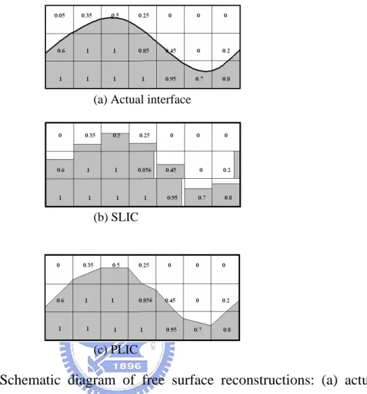
In CFD-ACE+ code, surface reconstruction is a prerequisite for determining the flux of fluid 2 from one cell to the next, and for determining surface curvatures when the surface tension model is activated. The following two approaches to surface reconstruction are currently available. z Single Line Interface Construction (SLIC) Method [23]

(45)

The original SLIC method approximates the interface in each mesh cell as a line that is parallel to one of the coordinate axes in a two-dimensional analysis, as shown in Fig. 2-8(b). However, the representation of the interface using SLIC is rough. The piecewise-linear interface calculation (PLIC) technique proposed by Youngs represents a useful refinement to the SLIC method using a straight line to approximate the interface in each computational cell, as displayed in Fig. 2-8(c). The PLIC method [25][26] is adopted and then coupled to the VOF method in this work.

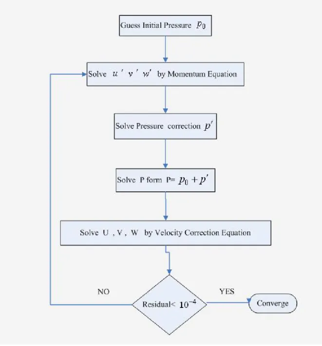
2.2.4 SIMPLEC algorithm

Solutions to the three momentum equations yield the three Cartesian components of velocity. Pressure-based approaches use the continuity equation to formulate an equation for pressure. In CFD-ACE+ code, SIMPLEC scheme is adopted. SIMPLEC stands for Semi-Implicit Method for Pressure-Linked Equations Consistent, and represents an enhancement of the well known SIMPLEC algorithm. SIMPLEC originally was proposed by Doormaal et al. in 1984 [27], an equation for pressure-correction is derived from the continuity equation. It is an inherently iterative method. Fig. 2-9 summarizes the SIMPLEC procedure.

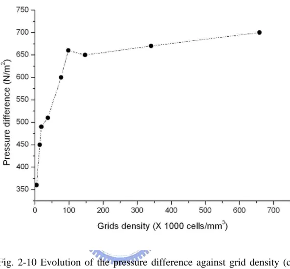
2.3 Grid density

The meshing elements and accuracy of the numerical model was determined by the testing of grid density. The convergence criteria of

(46)

the left and right interfaces, which is the pumping pressure for the motion of the liquid droplet. According to Fig. 2-9, the pressure difference reached a stable value, 650 N/m2, at a grid density of 150,000 cells/mm3, which was used in the simulation.

(47)

(48)

Fig. 2-3 Illustration of basic model used to deduce equations [14]

(49)

Fig. 2-5 Illustration of deducing pressure difference

(50)

(51)

(a) Actual interface

(b) SLIC

(c) PLIC

Fig. 2-8 Schematic diagram of free surface reconstructions: (a) actual interface; (b) SLIC approximation; (c) PLIC approximation

(52)

(53)

Fig. 2-10 Evolution of the pressure difference against grid density (case 05)

(54)

CHAPTER 3 ELECTRODE DESIGNS AND DEVICE

PROCESS

It is well-known that for EWOD, the drag of droplet is greater when the channel height becomes smaller. In order to solve this problem, a set of new shape of electrodes with extended rectangles was designed. The difference between the new and original electrodes can be seen in Fig. 3-1, in which the original one is square, whereas the new one is interdigitated with an “extended rectangle”. According to Eq. (2.22), the large pressure difference can move the droplet fancily. So the first step is to design the electrode that can generate large pressure difference. Consequently, the electrode shape and channel height are also needed to take into consideration. The comparison of the original electrodes with new ones will be discussed in next chapter.

3.1 Designs of electrode arrangements

All designed types of electrodes are illustrated in Fig. 3-2. There are nine types of electrodes with different widths of extended electrode, various areas of extended electrode and specific numbers of extended electrode. All of them are summarized in Table 3-1. Fig. 3-3 shows the arrangements of different electrodes, in which the first group is A1and A2, the second group is A3 and A4, the third group is A5 and A6, and the forth group is A7 and A8. For instance, the first group stands for the kind of electrode array in one-dimension, such as A1A2A1A2…. Similarly, the other three groups have the same meaning of first group, such as A3A4A3A4…, A5A6A5A6… , A7A8A7A8…, etc..

(55)

Table 3-1 Electrode shapes

Type Area of main electrode Area of extended electrode Width of extended electrode Number of extended electrode A1 0.3mm X 0.48mm 0.1mm X 0.08mm 0.08mm 2 A2 0.3mm X 0.48mm 0.1mm X 0.08mm 0.08mm 3 A3 0.3mm X 0.48mm 0.1mm X 0.02mm 0.02mm 2 A4 0.3mm X 0.48mm 0.1mm X 0.02mm 0.02mm 3 A5 0.3mm X 0.48mm 0.1mm X 0.05mm 0.05mm 2 A6 0.3mm X 0.48mm 0.1mm X 0.05mm 0.05mm 3 A7 0.3mm X 0.475mm 0.1mm X 0.025mm 0.025mm 5 A8 0.3mm X 0.475mm 0.1mm X 0.025mm 0.025mm 6

3.2 Experiment Setup

The experimental equipments consist of the contact angle goniometer, microscope, CCD camera and controlled circuit (microcontroller). The schematic configurations are shown in Fig. 3-4. The contact angle goniometer, whose base is on a XYZ platform, is used to measure contact angle on the hydrophobic layer (Teflon layer). The microscope is used to observe droplet motion, such as droplet moving, cutting, velocity and so on, recorded by CCD camera (30 frames/second) and subsequently transferred to the computer. The controlled circuit uses the input of digital signal to control electrodes, switching on or off on the EWOD device, which will be illustrated as follows. The photolithographic mask for EWOD device is shown in Fig.3-5.

(56)

3.2.1 Process of EWOD device

A metal layer of 200/800Ao Cr/Au was evaporated on glass substrate by E-beam Evaporator. After etching process and re-clean step of glass, SiNx thin film 3000Ao is deposited as the dielectric layer of EWOD by PECVD. The next step, photolithography is used to open the bonding pads, and dielectric layer on the bonding pads is removed by dilute buffered oxide etchant (BOE). At last, Dupont Teflon, diluted with 3M FC-77, is spun on the glass by spin coater to complete the fabrication.

Followings are the detailed recipe for fabrication of the above process, which is shown in Fig. 3-6 as well. The top plate process is illustrated in Fig.3-7. Figure 3-8 shows the SEM photo of EWOD device.

(I) Glass substrate process

1. Clean substrate in Caro acid ( H2SO4 : H2O2 = 3 : 1) at 120oC for 600

secs Æ Immerse the substrate in the deionized (D.I.) water for 60 secs Æ Blow and dry the substrate by N2 gun Æ Put soft bake on hot plate at

100oC_{for 180 sec.}

2. Metal evaporation, E-beam Evaporator, Cr/Au 200/800Ao .

3. Clean the glass in Acetone (ACE) with ultrasonic vibrator for 900 sec. 4. Soft bake on hot plate at 100oC for 180 sec.

5. Spin coat HMDS, 4000 rpm for 40 sec. 6. Soft bake on hot plate at 100oC for 180 sec.

7. Spin coat Shipley S1818 PR, 500 rpm for 15sec, 4000 rpm for 30sec. 8. Soft bake on hot plate at 100oC for 180 sec.

9. Exposure, Single-Side Mask Aligner.

10. Develop with Shipley MF 315 developer around 20 sec to window above bonding pads.

(57)

11. Hard bake on hot plate at 120oC for 600 sec.

12. Wet etching in potassium iodine solution to remove the Au for 4~8 sec. 13. Wet etching in Chromium Photomask Etchant to remove the Cr for 5 sec.

14. Clean the glass in Acetone (ACE) with ultrasonic vibrator for 300 sec, remove the photoresist.

15. Soft bake on hot plate at 100oC for 180 sec. 16. Deposit the Si3N4 by PECVD.

17. Spin coat diluted Teflon AF on the EWOD devices, 500 rpm for 15 sec, 3000 rpm for 30 sec.

18. Hard bake on hot plate, 110oC for 600 sec, 160oC for 1200 sec, and 260oC for 1800 sec.

(58)

(II) Silicon wafer substrate process

1. Clean substrate in Caro acid ( H2SO4 : H2O2 = 3 : 1) at 120oC_{for 600}

sec Æ Immerse the substrate in the deionized (D.I.) water for 60 sec Æ Blow the substrate dry by N2 gun Æ Soft bake on hot plate at 100oC_for

180 sec.

2. Deposit SiO2 (3000Ao ) and SiNx (3000Ao ) on the Si-wafer by PECVD. 3. Metal evaporation, E-beam Evaporator, Cr/Au 200/800Ao .

4. Clean the glass in Acetone (ACE) with ultrasonic vibrator for 900 sec. 5. Soft bake on hot plate at 100oC for 180 sec.

6. Spin coat HMDS, 4000 rpm for 40 sec. 7. Soft bake on hot plate at 100oC for 180 sec.

8. Spin coat Shipley S1818 PR, 500 rpm for 15sec, 4000 rpm for 30sec. 9. Soft bake on hot plate at 100oC for 180 sec.

10. Exposure, Single-Side Mask Aligner.

11. Develop with Shipley MF 315 developer around 20 sec to window above bonding pads.

12. Hard bake on hot plate at 120oC for 600 sec.

13. Wet etching in potassium iodine solution to remove the Au for 4~8 sec. 14. Wet etching in Chromium Photomask Etchant to remove the Cr for 5 sec.

15. Clean the glass in Acetone (ACE) with ultrasonic vibrator for 300 sec, remove the photoresist.

16. Soft bake on hot plate at 100oC for 180 sec. 17. Deposit the Si3N4 by PECVD.

18. Spin coat diluted Teflon AF on the EWOD devices, 500 rpm for 15 sec, 3000 rpm for 30 sec.

(59)

(III) Top plate process

1. Clean the ITO glass in Acetone (ACE) with ultrasonic vibrator for 600 sec. 2. Spin coat diluted Teflon AF (

0

1000Α_{) on the ITO glass, 500 rpm for 5 sec,}

500 rpm for 15 sec, 3000rpm for 5sec and 3000 for 40sec.

3.2.2 Measurement of contact angles

Measurements of the contact angle change by EWOD were made in a DI water droplet using Contact Angle Goniometer (MagicDrop, USA). The 10ul droplet was placed on a 3000 Å dielectric layer of silicon nitride coated with 1000 Å Teflon. A wire was penetrated into the droplet from the top, and the ac potentials with 1 K, 3K, 5K, 7K and 9K Hz, were applied between the liquid and the electrode underneath the dielectric layers. The contact angle was changed from 116° to 76°. The dielectric layers of nitride and Teflon formed two plate capacitors in series. The capacitance of a single capacitor is given by, 0 r c d ε ε = (3.1) where c is the capacitance per unit area. The equivalent capacitance of two

(60)

The dielectric constant (εr_{) of 3000 Å nitride and 1000 Å Teflon is 7.8 and 2,}

respectively. The equivalent capacitance of the nitride and Teflon layers can be obtained by Eq. (3.1) and (3.2). Fig. 3-9 shows the comparison of the experimental and theoretical contact angles based on Eq. (2.14). The contact angle parabolically decreases as the applied potential increases until it is saturated between 65° and 80°. The reason for the saturation is not clearly understood as of today. In any case, there exists a limitation in the contact angle change by EWOD, beyond which the higher potential can no longer decrease the contact angle any further. In addition, the Lippmann-Young’s equation does not consider the proceeding of the droplet. However, the droplet is advancing by the applied voltage. In order to produce larger pressure difference and to fit the simulation conditions, the voltage 100 AC with 3K or 5K Hz is used in the experiments. If a large voltage (> 110V) is applied to droplet, it will cause hydrolysis easier. Due to the limitation of microcontroller, the offset of voltage is set to 50V.

(61)

0.08mm

0

(62)

A1 A2 A3 A4 A5 A6 A7 A8 A9 Fig. 3-2 Different shapes of electrode

(63)

(64)

(a) Contact angle goniometer (b) Microscope and CCD came

(c) Controlled circuit (d) EWOD device Fig. 3-4 Illustration of experiment equipments

(65)

(a)

(b)

(c)

(d)

Fig. 3-5 (a) The pattern of 1-D photolithographic mask; (b)(c)(d) The pattern of pictures of EWOD control electrodes

(66)

（a）Acid washing （b）Metal deposition (Cr/Au)

(c) Photolithography (EWOD pattern) (d) Ache-down (Au/Cr)

(e) Nitride deposition (f) Spin coat Teflon

(Ⅰ) Glass substrate process Si3N4 S1818 Glass Au 800 0 A Cr 200 0 A Teflon 1000 0 A

(67)

Si wafer

（a）MRCA (Modified RCA Clean) （b）SiO2 and SiNx deposition

（c）Metal deposition (Cr/Au) (d) Photolithography (EWOD pattern)

(e) Ache-down (Au/Cr) (f) Nitride deposition

(g) Spin coat Teflon

Si3N4 3000 Å SiO2 3000 Å Cr 200 0 A Au 800 0 A S1818 Si3N4 Teflon 1000 0 A

(68)

(a) ITO glass (b) Spin coat Teflon

Fig. 3-7 Illustration of top plate process

Fig. 3-8 The SEM photo of EWOD device

Si3N4 3000 0 A SiO2 3000 0 A Cr 200 0 A Silicon Au 800 0 A ITO glass Teflon 1000 0 A ITO glass

(69)

(70)

CHPATER 4

RESULTS AND DISCUSSION

In this chapter, it will firstly present the simulation results that show the variations of droplet shapes under different pressure due to the electrode arrangement, the mean moving velocity of droplet and the time needed from one pattern to another while droplet is in the moving or cutting state. For experiments, it presents that a nano-liter droplets is created by different designs of square-, interdigiated- (2323) and interdigitated-electrode (5656). Finally, a comparison between numerical and experimental results for moving droplet is given.

4.1 Simulation

4.1.1 Simulation parameters

The initial conditions are the droplet location, droplet volume (radius of droplet) and initial velocity of droplet. In order to further simplify the problem, it assumes that the droplet radius is fixed at 0.3 mm for each simulation case. Because the channel height is one of the varying parameters, the resultant droplet volume (πr2×h

) is also changed. The corresponding values are list in Table 4-1.

Table 4-1 Volume of droplet (radius is 0.3 mm)

Channel height (h; μm) 20 35 70 Volume (nl) 5.655 9.896 19.792

Boundary conditions are the contact angles, which were obtained by experimental measurements under applied voltage. Other properties, which

(71)

are listed in Table 4-2, are composed of the gap between adjacent patterns, surface tension, gas viscosity, gas density, liquid viscosity and liquid density. In this study, the varying parameters are the channel height and the arrangement of electrodes, which were discussed briefly in the previous section. Consequently, the droplet location in Z direction in Table 4-2 is a function of channel height. The arrangement of electrodes was described in last chapter.

Table 4-2 Simulation properties

droplet location (m) X=1.5E-4, Y=2.4E-4, Z=variable, 1E-5, 1.75E-5 and 3.5E-5

radius of droplet (m) 3E-4

initial velocity of droplet (m/s) Vx=0, Vy=0 and Vz=0

contact angle 80°( wettability); 115°(non wettability)

electrode size (mm2)

0.5 X 0.48 (2323) 0.5 X 0.475 (5656) 0.5 X 0.5 (square)

main electrode area (mm2) 0.144 channel height (μm) Variable (20, 35 and 70)

gap of adjacent patterns (μm) 20 surface tension (N/m) 0.719 gas viscosity (air) (Kg/m⋅s) 1.846E-5 gas density (air) ( 3

/ m

Kg ) 1.1614

(72)

In this work, 16 simulation cases, which are based on the combinations of newly designed electrodes mentioned in Section 3-1, for both droplet moving and cutting. They are discussed as follows.

4.1.2 Droplet moving

In this section, the resultant mean velocities (V1 ) and pressure

differences (ΔP1) for each case are presented in Table 4-3 while the droplet

moves among adjacent electrodes. In this table, “a” represents the area sum of the extended rectangles and “A” total electrode area, whose representations can be seen graphically in Fig. 4-1. P1 is the initial pressure, P2 the instantaneous pressure as droplet starts to move and P3 the steady pressure as the droplet finish the movement. T and W are the time of moving among adjacent electrodes and the width of extended rectangle, respectively.

改善EWOD 元件於產生奈升級液滴之研究

國 立 交 通 大 學

機械工程學系

碩士論文