國 立 交 通 大 學
電子工程學系電子研究所
碩 士 論 文
應用於正交分頻多工技術為基礎之
無石英無線近身網路同步器
Synchronization Method for
Crystal-less OFDM-based
Wireless Body Area Network Applications
研究生 : 馬曉涵
指導教授 : 李鎮宜博士
應用於正交分頻多工技術為基礎之
無石英無線近身網路同步器
Synchronization Method for Crystal-less OFDM-based
Wireless Body Area Network Applications
研 究 生: 馬曉涵 Student: Hsiao-Han Ma 指導教授: 李鎮宜博士 Advisor: Dr. Chen-Yi Lee
國立交通大學
電子工程學系電子研究所
碩士論文
A Thesis
Submitted to Department of Electronics Engineering & Institute Electronics College of Electrical and Computer Engineering
National Chiao Tung University in Partial Fulfillment of Requirements
for the Degree of Master in
Electronics Engineering July 2009
應用於正交分頻多工技術為基礎之無石英
無線近身網路同步器
研 究 生: 馬曉涵 指導教授: 李鎮宜教授 國立交通大學電子工程學系電子研究所摘要
在本篇論文裡,介紹一個正交分頻多工系統的同步方法,應用於無石英震盪器之無 線近身網路,來增加整個系統收發端的頻率誤差容忍度。 無線近身網路為主的健康照護的系統越來越受人們的重視,尤其是針對人體生醫訊 號的偵測,可降低醫療成本以及提高醫療成效。應用情境如配戴在身上的無線感測器對 人體訊號做長時間的偵測,並以無線的方式將資料傳送給整合在手機或個人數位助理的 接收端。基於這樣的一個應用,極低的功率消耗跟高度整合的面積會是系統不可或缺的 需求,因此我們使用了互補式金屬氧化層半導體震盪器取代傳統產生系統時脈的石英震 盪器,以降低系統功率消耗以及提升整合度。 無石英震盪器現階段技術尚未成熟,使用此系統會造成收發段頻率誤差大的問題, 造成整個系統收發資料損失。於是本篇論文提出了一種套用於正交分頻多工的基頻同步 演算法配合一個可以調整的數位控制震盪器已達到減少收發端頻率誤差的效果。 將晶體振盪器整合進單一晶片中,可以降低系統的製造成本、面積及功率消耗。在 本篇論文我們對整個正交分頻多工無線近身網路系統的行為做一個詳盡的闡述,並分析 頻率校準的基頻演算法,最後建立了一個正交分頻多工的基頻原型來驗證這樣的行為。 這個方法套用在此論文之應用系統可使整個系統的頻率誤差容忍度拓展為140 倍,進而 達到小面積,低功率,高整合度的基頻系統晶片設計。Synchronization Method for
Crystal-less OFDM-based
Wireless Body Area Network Applications
Student: Hsiao-Han Ma Advisor: Chen-Yi Lee Department of Electronics Engineering and Institute of Electronics,
National Chiao-Tung University
Abstract
In this thesis, we propose a synchronization method for crystal-less OFDM-based wireless body area network (WBAN) applications to enlarge the frequency error tolerance between the transmitter and receiver.
WBAN systems for ubiquitous health monitoring are gradually attracting many attentions. This can reduce the medical cost and improve medical treatment outcomes. The wireless sensor node (WSN) nodes are placed on the human body allowing long-term health monitoring. Those gathered signals from a multiple of WSNs are wirelessly transmitted to a remote central processing node (CPN), such as mobile phone or PDA. Based on these applications, low power and highly integration properties are indispensable. To meet these needs, the CMOS oscillator is applied instead of the conventional quartz crystal oscillator.
However, the crystal-less technology does not come to maturity. It causes large frequency error in the system using the crystal-less oscillator. We propose a synchronization method for OFDM-based WBAN systems. Applying the crystal-less oscillator in the system, the area and power can be reduced a lot. In this thesis, a complete WBAN system and the novel synchronization algorithm are described. An OFDM emulation system is also established. In our application system, the overall frequency error tolerance is expanded to 140x, enabling the tiny area and highly integration SOC design.
誌謝
在Si2 實驗室的碩士班研究過程中,讓我學到了非常多的東西,過程相當充實。在 碩班的日子裡,幾乎每天待在實驗室的時數平均超過14 小時,假日也還是在實驗室過, 但還是樂此不疲。 首先要感謝我的指導教授李鎮宜博士,提供了非常完善的研究環境與資源,時常給 我們諄諄教誨。感謝實驗室的鍾菁哲學長,學長不遺餘力的為實驗室貢獻了很多很多, 如果沒有學長教導我們tapeout 的 flow,就不會有現在實驗室的豐碩的成果。 再來要感謝WBAN Group 的大學長,游瑞元學長,在碩士班裡給我的關心與指導。 雖然學長相當嚴厲,但從學長身上學習到許多強者的處事態度以及經驗。 再來要感謝實驗室的學長及同學們,感謝厲害的阿龍學長和義閔學長,常常給予我 鼓勵和關心,也解決我們許多技術上的問題。感謝已畢業的上賓學長,學長在我碩班的 期間教導了我許多知識,也從學長身上學到整理資料的好習慣。感謝畢業的 95 級學長 姐們,俊廷,冠麟,茗智,琇茹,清峰,在實驗室相當照顧我,即使在畢業後也常給我 打氣。感謝建螢學長,學長就像我的父親一般,除了在研究上的指導外也教導我許多待 人處世的道理。感謝燦文學長,在我困惑時給我很好的意見提點。感謝智超學長,在我 難過時總是為我加油打氣。感謝偉豪和書餘,大家一起討論功課和研究,互相學習,一 起進步。 最後還要感謝我的父母和兄長總是給予我的關心與鼓勵,讓我能夠盡全力的花費碩 班的生活在研究和學習上。在大家的支持下,我才能順利地完成碩士學業,最後感謝口 試委員的指導與寶貴的意見。CONTENTS
PAGE
摘要 ………..… I Abstract ……….…II 誌謝 ……… III CONTENTS ……… IV LIST OF FIGURES ………..…… VIII LIST OF TABLES ……….. XI
Chapter 1 ... 1
Introduction ... 1
1-1 Introduction to WBAN Systems ... 1
1-2 Introduction to Crystal-less Systems ... 2
1-3 Motivation... 5
1-4 Design Target ... 7
1-5 Outline of the Thesis ... 8
Chapter 2 ... 9 Application System ... 9 2-1 Overview... 9 2-2 System Behavior ... 10 2-2-1 Downlink ... 11 2-2-2 Uplink ... 12 2-3 Packet Format ... 12 2-3-1 Short Preamble ... 12 2-3-2 Long Preamble... 15 2-3-3 Packet Format ... 17
2-4 WiBoC System Block Diagram ... 18
2-4-1 Wireless Sensor Node... 19
2-4-2 Central Processing Node ... 20
2-5-1 AWGN ... 21
2-5-2 Carrier Frequency Offset ... 22
2-5-3 Sampling Clock Offset ... 27
2-5-4 Link Budget ... 28
2-6 Frequency Allocation ... 31
Chapter 3 ... 32
Synchronization PAFEE Method ... 32
3-1 PAFEE -- Packet Detection Algorithm ... 32
3-1-1 Conventional Algorithm ... 32
3-1-2 Proposed Algorithm... 34
3-2 PAFEE -- Frequency Error Estimation Algorithm... 45
3-2-1 Conventional Algorithm ... 46
3-2-2 Proposed Algorithm... 47
3-3 PAFEE Method Flow ... 50
Chapter 4 ... 52
Simulation Results and Performance Analysis... 52
4-1 Simulation on PAFEE -- Packet Detection ... 52
4-1-1 ROC Curves... 52
4-1-2 Detection Rate, False Alarm Rate Versus SNR ... 57
4-1-3 Detection Rate Versus Frequency Error ... 59
4-2 Simulation on PAFEE -- Frequency Error Estimation... 61
4-3 Simulation on System PER Performance ... 64
Chapter 5 ... 67
Hardware Implementation... 67
5-1 Overall Architecture... 67
5-1-1 Packet Detector... 67
5-1-2 Phase Rotator... 69
5-1-3 Frequency Error Estimator ... 71
5-2 Simulation on Quantization Results... 73
5-2-1 Simulation on PAFEE -- Packet Detection... 73
5-2-3 Simulation on System PER Performance ... 77
5-3 Hardware Overhead ... 78
Chapter 6 ... 81
Emulation of Crystal-less Baseband System... 81
6-1 Building Block ... 81
6-2 Evaluation System ... 82
6-3 Emulation Results ... 84
Chapter 7 ... 88
Conclusions and Future Work ... 88
7-1 Conclusions... 88
7-2 Future Work ... 90
References ... 92
Appendix A ... 95
Embedded Crystal Design... 95
A-1 Introduction... 95
A-2 Proposed DCO ... 97
A-2-1 DCO Architecture ... 97
A-2-1 Coarse-tuned Stage ... 97
A-2-2 Fine-tuned Stage ... 99
A-3 Measurement Results ... 101
A-3-1 Coarse-tuned Stage ... 102
A-3-2 Fine-tuned Stage ... 104
A-4 System Comparison ... 107
A-5 Conclusion ... 108
Appendix B ... 109
IP Deliverable... 109
B-1 Overall Architecture ... 109
B-2-1 Components ... 110
B-2-3 External Signal Descriptions... 111
B-2-3 FSM... 113
B-2-4 Area ... 114
B-2-5 Power ... 115
B-3 Architecture of Transmitter ... 117
B-3-1 Components ... 117
B-3-2 External Signal Descriptions... 118
B-3-3 FSM... 119
B-3-4 Area ... 119
LIST OF FIGURES
PAGE
Figure 1-1: Motivation, pros and cons ... 6
Figure 1-2: Motivation and PAFEE method... 6
Figure 2-1: The target operation scenario of WBAN system... 10
Figure 2-2: WiBoC system behavior... 10
Figure 2-3: WiBoC system device connection behavior... 11
Figure 2-4: Short preamble format... 13
Figure 2-5: Preamble format with 24-tone in frequency domain... 14
Figure 2-6: Preamble format with 6-tone in frequency domain... 15
Figure 2-7: Long preamble format in time domain... 17
Figure 2-8: Downlink packet format... 18
Figure 2-9: Uplink packet format... 18
Figure 2-10: WSN block diagram ... 20
Figure 2-11: CPN block diagram ... 21
Figure 2-12: CFO effect ... 23
Figure 2-13: mathematical CFO model... 26
Figure 2-14: MATLAB CFO model... 27
Figure 2-15: SCO effect ... 28
Figure 3-1 (a): ROC curves from mathematics deduction ... 44
Figure 3-1 (b): ROC curves from mathematics deduction (Zoom-in) ... 44
Figure 3-2: ROC curves under different M ... 45
Figure 3-3: Frequency error estimation block... 50
Figure 3-4: Synchronization PAFEE algorithm flow ... 51
Figure 4-1(a): Frequency error estimation block ... 53
Figure 4-1(b): Frequency error estimation block (Zoom-in) ... 54
Figure 4-3: ROC curves in different L ... 56
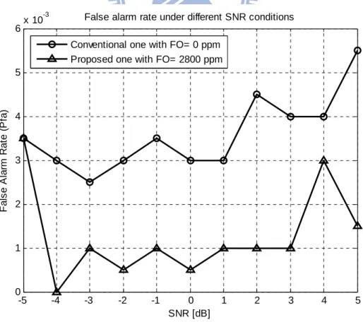
Figure 4-5: Detection rate in conventional one and proposed one... 58
Figure 4-6: False alarm rate in conventional one and proposed one... 58
Figure 4-7: Detection rate under different CFO and SCO conditions, SNR=1 dB... 59
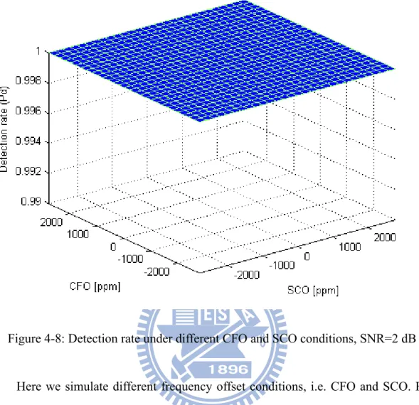
Figure 4-8: Detection rate under different CFO and SCO conditions, SNR=2 dB... 60
Figure 4-9: Detection rate under different FO and SNR conditions ... 61
Figure 4-10: Estimation corrent rate versus frequency error ... 62
Figure 4-11 (a): Maximum remaining error versus frequency error ... 63
Figure 4-11 (b): Maximum remaining error versus frequency error (Zoom-in) ... 63
Figure 4-12: Packet error rate versus SNR, N=3 ... 65
Figure 4-13: Packet error rate versus SNR, N=1 ... 66
Figure 5-1: Overall architecture of WSN system... 67
Figure 5-2: Hardware architecture of packet detector... 68
Figure 5-3: Hardware architecture of moving average ... 69
Figure 5-4: Hardware architecture of phase rotator in packet detection state... 69
Figure 5-5: Hardware architecture of phase rotator after detecting the packet... 71
Figure 5-6: Hardware architecture of frequency error estimator ... 72
Figure 5-7: Real part of the Ri, i is from 1 to 16... 72
Figure 5-8: Imaginary part of the Ri, i is from 1 to 16... 73
Figure 5-9: Fixed point ROC curves ... 74
Figure 5-10: Fixed point detection rate under different frequency error condition ... 75
Figure 5-11: Fixed point estimation correct rate versus frequency error ... 76
Figure 5-12: Fixed point maximum remaining error versus frequency error ... 77
Figure 5-13: Fixed point packet error rate versus SNR ... 78
Figure 6-1: Hardware emulation building blocks ... 81
Figure 6-2: Evaluation system... 82
Figure 6-3: Received signal shown in spectrum analyzer... 84
Figure 6-4: Estimation results with frequency error 0, 400, 800, 1200 ppm ... 86
Figure 6-5: Estimation results with frequency error 1600, 2000, 2400, 2800 ppm ... 87
Figure A-2: Coarse-tuned stage... 98
Figure A-3: Schmitt trigger cell ... 99
Figure A-4: Fine-tuned stage... 101
Figure A-5: The period of DCO in coarse-tuned stage ... 103
Figure A-6: The RMS jitter of DCO in coarse-tuned stage... 103
Figure A-7: The period of DCO in fine-tuned stage ... 105
Figure A-8: The RMS jitter of DCO in fine-tuned stage... 106
Figure B-1: Overall architecture of WSN system ... 109
Figure B-2: FSM of WSN_RX... 113
Figure B-3: P&R view of WSN_RX... 115
Figure B-4: FSM of WSN_TX... 119
LIST OF TABLES
PAGE
Table 1-1: The power consumption, area, and cost of the quartz crystal [11]... 3
Table 1-2: Existing solutions for crystal-less communications systems ... 4
Table 1-3: Candidate clock source in CMOS technology ... 4
Table 1-4: WBAN system with their allowable frequency errors ... 5
Table 1-5: Design target ... 7
Table 2-1: Link Budget ... 30
Table 5-1: Area overhead ... 79
Table 5-2: Power overhead... 80
Table 6-1: Baseband components... 83
Table 6-2: The relationship between frequency error and clock period... 85
Table 7-1: System comparison summary ... 89
Table 7-2: WiBoC OFDM system summary ... 90
Table A-1: Delay element in coarse-tuned stage ... 99
Table A-2: Delay element in fine-tuned stage... 101
Table A-3: DCO in coarse-tuned stage... 104
Table A-4: DCO in fine-tuned stage... 106
Table A-5: DCO power consumption under different supply voltage... 107
Table A-6: DCO performance comparison... 108
Table B-1: The component in WSN_RX... 110
Table B-2: Mode of operation in WSN_RX... 111
Table B-3: External signal description in WSN_RX... 112
Table B-4: State description in WSN_RX... 114
Table B-5: Area reports in WSN_RX... 114
Table B-6: Power classification and definition ... 116
Table B-7: Power report in WSN_RX... 116
Table B-8: The component in WSN_TX... 117
Table B-10: External signal description in WSN_TX... 118
Table B-11: State description in WSN_TX ... 119
Table B-12: Area report in WSN_TX... 120
Chapter 1
Introduction
1-1 Introduction to WBAN Systems
With the progress of the medical technology, there are more and more accurate and higher-level instruments invented in the hospitals. These devices help human to observe their disease in early time. The doctor will prevent and cure the disease efficiently.
In recently years, the ubiquitous healthcare devices are presented to the public and explode to be popular. Ubiquitous healthcare monitoring plays a crucial role in body signal tracking and recording. The patients want comfortable and portable devices to examine their physical status. This device is not only portable and convenient, but extends medical services from an indoor room to any open roaming spaces.
The wireless body area network (WBAN) is designed for the applications of body signal gathering and monitoring to provide reliable physical information. It is composed by a multiple of wireless sensor nodes (WSN), and a central processing node (CPN). The WSN is capable of sampling, processing, and communicating the body information to the CPN. These nodes are placed on the human body as tiny patches. They are comfortable and convenient for human to observe their physical status in any time from the CPN. The CPN is built in some portable devices, such as PDA, cell phones, or personal laptop.
Existing solutions for the WBAN applications could be found in [1-5]. The well-defined systems, e.g. Bluetooth [1] and Zigbee [2], are designed for widespread applications, including entertainment, positioning, factory product management, and healthcare. With the increasing demands in wireless body area applications, however, these two candidate systems have difficulties to meet the consumer electronic devices functions and the healthcare at the same time.
There are also some customized systems, MIThrils [3], CodeBlue [4], and Human++ [5], are explored for WBAN system constructions in body-oriented applications.
It is our intention to design WBAN systems to be tiny and low power. To achieve the target, the crystal replacement method is used. It is called crystal-less system if the system does not have a crystal oscillator as its clock source.
1-2 Introduction to Crystal-less Systems
With the progress of the system on chip (SoC) technology, the most of the circuits in a system can be integrated in one chip. Applying the SoC technology in communications system is very attractive. Nowadays the baseband circuits are integrated in one chip except the clock source, a crystal oscillator.
Though the crystal oscillator plays an important role for system clock, it boosts the effort in system integration. The quartz crystal consumes a lot of power and occupies large area in the chip, as shown in Table 1-1 [11].
Table 1-1: The power consumption, area, and cost of the quartz crystal [11]
In-crystal 1μW~200μW Power
consumption Oscillator 1mW~50mW (active) 10μW~50μW (standby) SMD 3.2mm x 2.5mm x 0.5mm Area
DIP 11.5mm x 4.7mm x 3.5mm
Cost US$0.15~2
Wireless sensor nodes require transceivers that are small, cheap, and power efficient. To achieve better integration and less power, more cost-effective baseband chip applications, the crystal-less system is explored. One solution of the crystal-less system, which has a self-calibrated embedded crystal (eCrystal), is proposed by NCTU [6]. The eCrystal system uses its embedded clock generator instead of a crystal oscillator.
There are some existing customized solutions for crystal-less communications systems [7-10]. The CMOS circuits are used as a system reference clock in the chip, e.g. ring oscillator, digital controlled oscillator, and voltage controlled oscillator. The CMOS circuits are sensitive to the process, voltage, and temperature (PVT) variations. The customized solutions use some frequency-insensitive modulation to overcome the inaccuracy of system clock. The following table shows the modulation and oscillator design of the existing solutions for crystal-less communications systems. The initial error of the oscillator is large, i.e, above 1%.
Table 1-2: Existing solutions for crystal-less communications systems
Systems modulation oscillator design initial error
[7] ISCAS 2008 IR + PPM CMOS clock generator 1.1 %
[8] ISSCC 2008 OOK CMOS Ring Oscillator 2.5 %
[9] PIMRC 2006 BFSK voltage controlled oscillator 1 %
[10] ISSCC 2009 ASK Ring Oscillator N/A
In the proposed eCrystal system, the clock source is designed. Table 1-3 shows some candidates clock source made in CMOS technology. The LC tank oscillator is not suitable in our design due to its large frequency drift and large power. Though the MEMS oscillator has good properties about the frequency drift and power, it is not taken into consideration due to its non-standard process and long processing period.
The eCrystal method in NCTU has been proposed in self-defined system specification with generation frequency 5MHz and frequency drift 0.28%.
Table 1-3: Candidate clock source in CMOS technology
LC [31] MEMS [32] RO [33] eCrystal
Process CMOS CMOS/ MEMS CMOS CMOS
Fgen Carrier freq. 0.1~10GHz Wide 1.5~4GHz 7MHz 5MHz Frequency 10~15% ±0.03% ±2.65% ±0.28% Power 6~20mW 0.1mW 1.5mW 0.25mW
1-3 Motivation
To achieve the low-power and highly integrated ubiquitous healthcare monitoring applications, we apply the crystal-less technology in the WBAN system.
The communications systems need accurate clock generator, or the data won’t be correctly recovered in the receiver side. Table 1-4 shows the existing WBAN system and their allowable frequency error tolerance.
Table 1-4: WBAN system with their allowable frequency errors
Systems modulation Frequency Error Tolerance
[1] Bluetooth FHSS ±20ppm
[2] Zigbee DSSS ±40ppm
[3] MIThril FHSS ±30ppm
[4] CodeBlue DSSS ±25ppm
[5] Human++ UWB N/A
The allowable frequency error tolerance is very small, i.e, below 40ppm. The clock generator is designed with limited initial frequency offset, say 0.28%, under process, voltage, and temperature variations.
The target is to establish a standard compatible system with crystal replacement. The OFDM-based system is selected. Due to the low precision of the eCrystal oscillator, our motivation is to design a baseband calibration algorithm to detect the clock error and compensate the frequency mismatch between the transmitter and the receiver as shown in Figure 1-1.
Figure 1-1: Motivation, pros and cons
For the large clock error, the first problem encountered is that packet is undetectable. The algorithm of detecting the packet under large frequency error is proposed. After the packet detection, the frequency error is estimated and feedback to the clock generator. The algorithm is called packet detection and frequency error estimation (PAFEE) method, as shown in Figure 1-2.
A system defined as wireless body on the chip (WiBoC), based on the OFDM scheme is used as the evaluation platform in this thesis. The crystal-less system behavior and hardware design will be discussed and analyzed. The prototype platform is also established to verify the behavior of the overall system.
1-4 Design Target
In the self-defined crystal-less system, there is frequency drift 0.28% in our eCrystal clock generator. To solve the large frequency error and have the performance remain the same, we have to reach the design target as shown in Table 1-5.
Table 1-5: Design target
Conventional [12] Proposed PAFEE Frequency error
tolerance range 100 ppm 2800 ppm
Final accuracy 20 ppm 20 ppm
Detection rate 99.95% @ SNR ≥ 2dB 99.95% @ SNR ≥ 2dB False alarm rate < 0.05 % < 0.05 % Target
Estimation
correct rate > 0.9999 @ SNR ≥ 2dB > 0.9999 @ SNR ≥ 2dB
Short preamble 2.5 12
(Downlink only/ Once)
Estimation time 32 ms 153.6 ms Spec.
Requirement
We apply the 802.11a specification [12] in our WiBoC system as the conventional approach. The frequency tolerance range is 100 ppm. We have to meet the constraints of the detection rate, false alarm rate and estimation correct rate in our system with 2800 ppm frequency error condition. However, there are some requirements in the specification. The short preamble is designed strengthen.
In the following simulation, the SNR condition is set 2 dB for the packet error rate (PER) performance is 1 at SNR = 2dB. If we can guarantee the synchronization performance is stable in SNR=2 dB, the PER performance will remain the same.
1-5 Outline of the Thesis
The thesis is organized as follows. Chapter 2 introduces the application system, WiBoC, which is an OFDM-based WBAN system, including the overall system behavior and system specification. In Chapter 3, the proposed synchronization algorithm is presented. Chapter 4 shows the system simulation results of the proposed algorithm. The hardware implementation details are described in Chapter 5. Then the overall system emulation results are shown in Chapter 6. Finally, chapter 7 gives the conclusions and future work.
Chapter 2
Application System
2-1 Overview
In this chapter, the WiBoC system is introduced, which is the OFDM-based WBAN system. It is the evaluation platform in the thesis. The target operation scenario is shown in Figure 2-1.
The WBAN system contains one central processing node (CPN) and a multiple of wireless sensor nodes (WSN). The WSN gathers the physical information from the human body, such as EEG wave, ECG wave, glucose, blood pressure, and so on. It is capable of sampling, processing, and communicating, and presents as a tiny patch in human body. The gathered signals from a multiple of WSNs are wirelessly transmitted to a remote CPN, which is integrated in a portable device, such as mobile phone or PDA. Both the CPN and WSN have transmitter and receiver. They transmit and receive data to each other through downlink and uplink path.
For simplicity, the evaluation WiBoC system has one central processing node and one wireless sensor node in the thesis.
Figure 2-1: The target operation scenario of WBAN system
2-2 System Behavior
The WiBoC system behavior is shown in Figure 2-2. A successful transmission is divided into two parts, downlink and uplink. Here the downlink is defined as that CPN transmits preamble to WSN. The uplink is defined as both the preamble and data transmit from WSN to CPN. The downlink process will help WSN to detect the packet and estimate the frequency error by the packet information.
Figure 2-3 shows the system behavior in terms of time axis and system device connection. The body signals are gathered and transmitted from the WSNs. The CPN receives the human body signals from WSNs for ubiquitous monitoring. When the WSNs and CPN are activated, they are initially in a reset state. In the beginning of network establishment, the CPN waits for sign-in signals from possible WSNs. After all WSNs join this network, the CPN broadcasts packets to every WSN (downlink process) for timing and frequency synchronizations. After the network synchronization in the downlink process, each WSN starts to gather body signals and transmits to the CPN (uplink process). Finally, the CPN receives the body information from WSNs.
Figure 2-3: WiBoC system device connection behavior
2-2-1 Downlink
In the downlink process, the CPN transmits the downlink preamble to the WSN. The preamble is the known sequence transmitted from the CPN. The WSN is activated all the time after the reset. It detects the data from the downlink channel. The preamble is transmitted through the channel and is distorted under a variation of channel conditions. Once the packet is detected, the WSN uses the remaining
distorted received data to estimate the frequency error.
2-2-2 Uplink
After the downlink process, the clock source in WSN is tuned correctly. The frequency mismatch from the CPN to the WSN is eliminated. The WSN starts to gather the body signal and transmits to the CPN. In the uplink process, not only the data is transmitted, but the preamble is also added in front of the data and transmitted. Then the CPN receives the complete uplink data for the further inspections.
2-3 Packet Format
2-3-1 Short Preamble
The short preamble format is from the IEEE 802.11a [12] specification. It takes advantage of the properties of short preamble to do the synchronization and frequency error estimation. The short preamble format in frequency domain S(f) is shown in the Equation 2-1, S(f) = AS [ 0 0 0 0 -1-j 0 0 0 -1-j 0 0 0 1+j 0 0 0 1+j 0 0 0 1+j 0 0 0 1+j 0 0 0 0 0 0 0 0 0 0 0 0 0 0 0 1+j 0 0 0 -1-j 0 0 0 × 1+j 0 0 0 -1-j 0 0 0 -1-j 0 0 0 1+j 0 0 0 ], (2-1)
where AS is a scaling factor that is dependent on the front-end device. In the receiver side, AS varies by the auto gain control (AGC) of the analog to digital converter (ADC). From the Equation 2-1, the short preamble format can be regard as 12 tones in frequency domain. It is also observed that the short preamble s(t) in time
domain as expressed in Equation 2-2. The 16 of the 64 time domain data are shown, because the time domain of the short preamble is repeated sequence, i.e., s(1:16)=s(17:32)=s(33:48)=s(49:64). And as is also a scaling factor similar to the AS in Equation 2-1.
s(t) = ifft( S(f), 64 )
s(1:16) = as [ 0.0313 + 0.0313i -0.0900 + 0.0016i -0.0092 - 0.0533i 0.0970 - 0.0086i 0.0625 0.0970 - 0.0086i -0.0092 - 0.053
×
3i -0.0900 + 0.0016i 0.0313 + 0.0313i 0.0016 - 0.0900i -0.0533 - 0.0092i -0.0086 + 0.0970i 0 + 0.0625i -0.0086 + 0.0970i -0.0533 - 0.0092i 0.0016 - 0.0900i ],
(2-2)
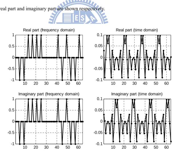
The short preamble in frequency domain and time domain are plot in Figure 2-4. The real part and imaginary part are shown respectively.
10 20 30 40 50 60 -1 -0.5 0 0.5 1
Real part (frequency domain)
10 20 30 40 50 60 -1 -0.5 0 0.5 1
Imaginary part (frequency domain)
10 20 30 40 50 60 -0.1 -0.05 0 0.05 0.1
Real part (time domain)
10 20 30 40 50 60 -0.1 -0.05 0 0.05 0.1
Imaginary part (time domain)
The frequency domain properties are good for us to estimate the frequency error. It has 12 tones in frequency domain. It repeated 4 times every 16 data in time domain. The repeated preamble is used to do the packet detection, and the remaining preamble is for the frequency error estimation. The preamble format is suitable in this algorithm. If the preamble that has 24 tones in frequency domain is used, the time domain data will be repeated 2 times every 32 data, as shown in Figure 2-5. If the preamble that has 6 tones in frequency domain, the time domain data will be repeated 8 times every 8 data, as shown in Figure 2-6.
10 20 30 40 50 60 -1 -0.5 0 0.5 1
Real part (frequency domain)
10 20 30 40 50 60 -1 -0.5 0 0.5 1
Imaginary part (frequency domain)
10 20 30 40 50 60 -0.2 -0.1 0 0.1 0.2
Real part (time domain)
10 20 30 40 50 60 -0.2 -0.1 0 0.1 0.2
Imaginary part (time domain)
10 20 30 40 50 60 -1 -0.5 0 0.5 1
Real part (frequency domain)
10 20 30 40 50 60 -1 -0.5 0 0.5 1
Imaginary part (frequency domain)
10 20 30 40 50 60 -0.05
0 0.05
Real part (time domain)
10 20 30 40 50 60 -0.05
0 0.05
Imaginary part (time domain)
Figure 2-6: Preamble format with 6-tone in frequency domain
If the 6-tone preamble format is selected as the short preamble, the repeated 8 data are used for packet detection. For the frequency domain information is not enough to estimate the frequency error, this short preamble is not applied in our system. If the 24-tone preamble format is selected as the short preamble, the repeated 32 data are used for packet detection. The 32 data is needed for packet detection, this will increase the preamble length and hardware overhead is raised. This is not appropriate in our system.
2-3-2 Long Preamble
The long preamble format is from the IEEE 802.11a [12] specification. It takes advantage of the properties of long preamble to perform the boundary detection and fine CFO estimation. The long preamble format in frequency domain L(f) can be expressed as Equation 2-3, where AL is a scaling factor that is depend on the
front-end device. L(f) = AL [0 1 -1 -1 1 1 -1 1 -1 1 -1 -1 -1 -1 -1 0 1 -1 -1 1 -1 1 -1 1 1 1 1 -1 1 -1 0 0 0 0 0 1 -1 1 1 1 -1 -1 1 1 -1 1 -1 1 × 1 0 1 1 1 -1 -1 1 1 -1 1 -1 1 1 1 1], (2-3)
The long preamble format in time domain l(t) is expressed as Equation 2-4, where al is also a scaling factor similar to the AL in Equation 2-3.
l(t) = ifft( L(f) )
= al [ 0.1250 -0.0082 - 0.1322i 0.0704 - 0.0899i 0.1059 + 0.0564i -0.0078 + 0.0544i 0.0451 - 0.1098i -0.0891 - 0.0405i -0.0185 - 0.1127i
×
0.0754 - 0.0259i 0.0292 + 0.0073i 0.0184 - 0.1175i -0.1092 - 0.0490i 0.0125 - 0.0512i 0.0288 - 0.0270i -0.0164 + 0.1741i 0.1503 - 0.0137i 0.0625 - 0.0625i 0.0058 + 0.1126i -0.0633 + 0.0086i -0.1014 + 0.1109i 0.0942 + 0.0372i 0.0420 + 0.0702i -0.0777 + 0.0346i -0.0323 + 0.0053i -0.0129 - 0.1509i -0.1417 - 0.0470i -0.1533 + 0.0383i 0.0898 - 0.1538i 0.0261 + 0.1428i -0.1010 + 0.0310i 0.0611 + 0.1713i 0.0153 + 0.0618i -0.1250 0.0153 - 0.0618i 0.0611 - 0.1713i -0.1010 - 0.0310i 0.0261 - 0.1428i 0.0898 + 0.1538i -0.1533 - 0.0383i -0.1417 + 0.0470i -0.0129 + 0.1509i -0.0323 - 0.0053i -0.0777 - 0.0346i 0.0420 - 0.0702i 0.0942 - 0.0372i -0.1014 - 0.1109i -0.0633 - 0.0086i 0.0058 - 0.1126i 0.0625 + 0.0625i 0.1503 + 0.0137i -0.0164 - 0.1741i 0.0288 + 0.0270i 0.0125 + 0.0512i -0.1092 + 0.0490i 0.0184 + 0.1175i 0.0292 - 0.0073i 0.0754 + 0.0259i -0.0185 + 0.1127i -0.0891 + 0.0405i 0.0451 + 0.1098i -0.0078 - 0.0544i 0.1059 - 0.0564i 0.0704 + 0.0899i -0.0082 + 0.1322i ],
(2-4)
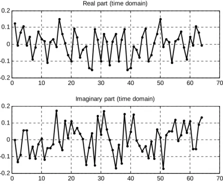
Figure 2-7 shows the long preamble format in time domain and frequency domain.
0 10 20 30 40 50 60 70 -0.2 -0.1 0 0.1 0.2
Real part (time domain)
0 10 20 30 40 50 60 70 -0.2 -0.1 0 0.1 0.2
Imaginary part (time domain)
Figure 2-7: Long preamble format in time domain
2-3-3 Packet Format
The packet comprises of short preamble, long preamble and the data. The preamble is in the head of the packet. The data is followed behind the preamble. Figure 2-8 shows the downlink broadcast packet. The first N repeated short preambles are used for the synchronization algorithm. The N depends on the simulation and the recursive times of the synchronization, and N is 3 in our approach. The following SGI is the half of the short preamble, which is regarded as GI of the short preamble. The LGI from the long preamble are for the boundary detection, which is the half of long preamble. The subsequent two long preambles are used to perform channel estimation and further fine frequency error estimation.
Figure 2-8: Downlink packet format
Uplink packet structure is shown in Figure 2-9. The preambles and the data are scrambled into a packet. The preamble is the same as the downlink one. It is used to perform symbol timing synchronization and symbol boundary detection. The following two long preambles are used for channel estimation. The final part of the packet is the payload data.
Figure 2-9: Uplink packet format
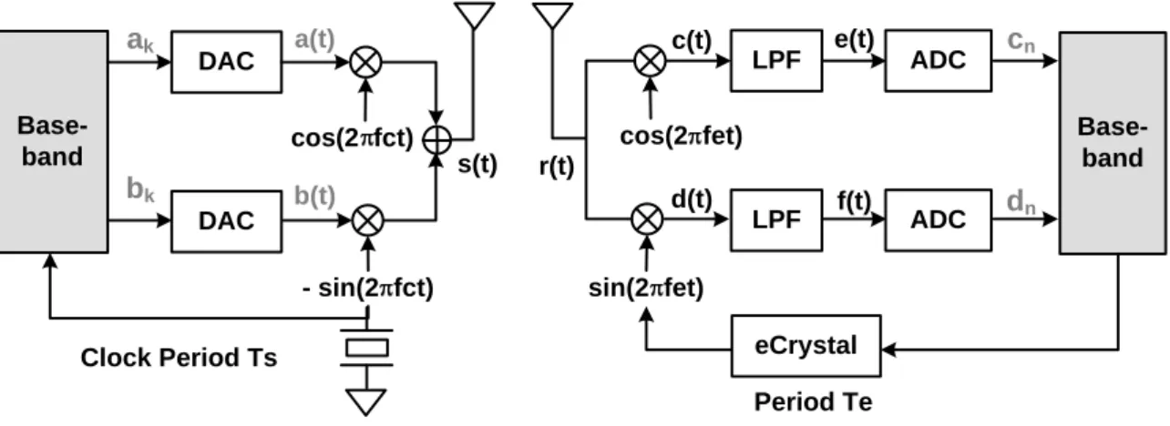
2-4 WiBoC System Block Diagram
The WiBoC system block diagram is introduced in this section. The WiBoC system consists of one WSN and one CPN. The operation of the CPN just sets for simulation. We put more emphasis on the WSN behavior and its hardware implementation in this thesis.
2-4-1 Wireless Sensor Node
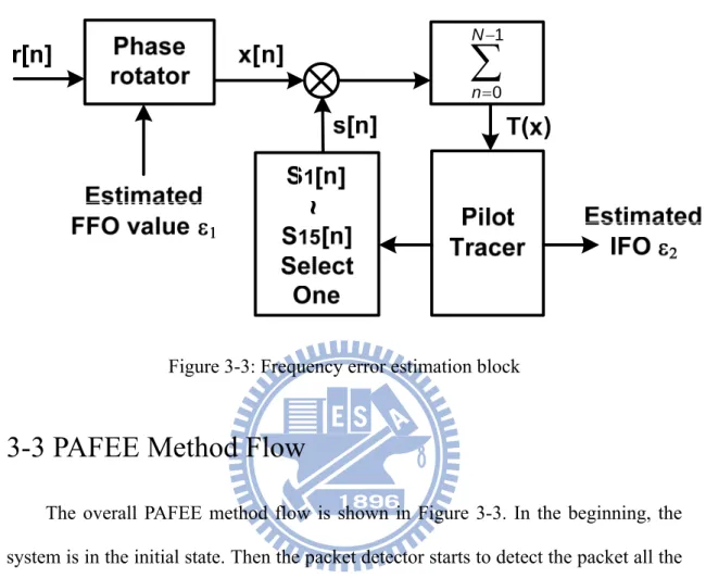
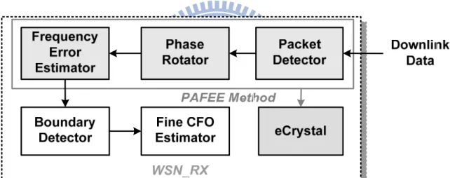
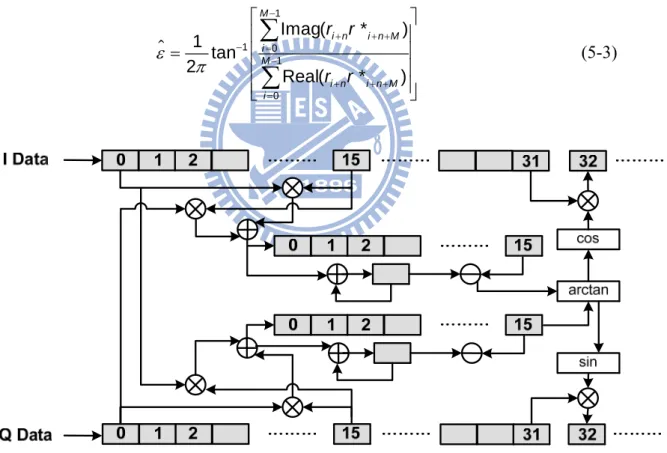
Figure 2-10 shows the block diagram of the WSN. In the downlink process, the WSN receives the downlink preamble from the CPN in the beginning. The packet detector detects the packet all the time after the reset state. Once the packet have detected, the phase rotator calculates the signal phase between two carriers and rotates the received signal. After the processing of the phase rotator, the frequency error estimator performs the frequency error detection during the time that receiving the short preamble.
The overall frequency error is the summation of the amount estimated by the phase rotator, the frequency error estimator, and fine CFO estimator. This estimation error amount is feedback to the eCrystal, which is the tunable clock generator. The clock generator will generate the accurate clock in a short period, and the data after the short preamble (i.e long preamble) will not be lost. Then the boundary detection and fine CFO estimation is operated.
After the clock is tuned accurately, WSN starts to gather the body signal to the uplink packet and transmits to the CPN. The body signal is encoded in FEC bitstream. The FEC encoder is convolutional encoder, which is designed with coding rate R=1/2, K=7, and generator polynomials g0=1338 and g1=1718. The FEC bitstream is
modulated in QPSK and then passed through IFFT block. After the IFFT and GI insertion, the packet is transmitted to the uplink channel.
The WSN is composed of one transmitter (WSN_TX) and one receiver (WSN_RX). The yellow part in Figure 2-10 is the block diagram of synchronization algorithm, PAFEE method.
D A C QPSK Mapper A D C IFFT Phase Rotator Packet Detector Fine CFO Estimator FEC Bitstream eCrystal
Wireless Sensor Node
R F Frequency Error Estimator Boundary Detector GI Insertion WSN_TX WSN_RX
PAFEE Method Syn.
Figure 2-10: WSN block diagram
2-4-2 Central Processing Node
In the CPN, the received data from the WSN have been pre-calibrated. The synchronizer detects the symbol timing with symbol correlation results. The synchronized data are then sent into the FFT block. After transformation, the phase recovery is performed to calibrate the data. Then the recovered data are demapped for later FEC decoding. The CPN clock diagram is shown in Figure 2-11.
Figure 2-11: CPN block diagram
2-5 Channel Model
The channel condition is important for the wireless communications systems. The system design depends on the channel conditions. In WBAN applications, the channel is assumed simple because its communication distance is short, i.e., smaller than 3 meter. We can ignore the multipath channel effect. In this section, three kinds of channel conditions are focused, additive white Gaussian noise (AWGN) channel, carrier frequency offset (CFO) and sampling clock offset (SCO).
2-5-1 AWGN
In the wireless channel, due to the thermal vibrations of atoms in antennas, shot noise, black body radiation, etc, the receiver can not receive identical signal from the transmitter. The phenomenon is called additive white Gaussian noise, say, AWGN. When the original signal pass through the AWGN channel, the linear addition noise is added to the signal. The additive noise is modeled as a Gaussian distribution. The AWGN generated by MATLAB can be expressed as Equation 2-5,
( ) / 20 ( ) (1, ) (1, ) 1 10 2 − = × + × × = × Pdata SNR w t randn L rms j randn L rms where rms (2-5)
The randn(1, L) returns an 1-by-L matrix containing random values from a normal distribution with mean zero and standard deviation one. The rms represents the normalized root mean square power of the coming L data. The Pdata is the power of
the data with unit dB.
2-5-2 Carrier Frequency Offset
Carrier frequency offset is caused by the frequency mismatch between the transmitter and receiver in the front-end device, i.e., synthesizer, modulator, and demodulator.
Take the short preamble in our system as the example, the following Figure 2-12 shows the frequency offset effect in frequency domain. The system operates in 1.4GHz radio band, and occupies 5MHz bandwidth. The frequency domain is comprehended in terms of 64-point FFT results. The x-axis represents the index from 1 to 64. The y-axis is the magnitude of the subcarrier. Consider the frequency allocation in RF band as the fixed window which is occupied from fc-BW/2 to fc + BW/2 in the frequency domain. The fc and BW represent the center frequency and the bandwidth respectively. The frequency offset effect is regarded as the data shift out of the window in the frequency domain. This phenomenon results in large amount data loss. From the Figure 2-12, the carriers are shifted left with the frequency that is proportional to the frequency offset amount. When the CFO = 3000 ppm, the carriers are shifted about 1.4GHz x 3000ppm = 4.2 MHz, which is close to the bandwidth 5MHz. There is no data in this window under such large frequency offset.
0 10 20 30 40 50 60 0 0.5 1 (1 ) CFO=0 ppm 0 10 20 30 40 50 60 0 0.5 1 (2 ) CFO=100 ppm 0 10 20 30 40 50 60 0 0.5 1 (3 ) CFO=200 ppm 0 10 20 30 40 50 60 0 0.5 1 (4 ) CFO=500 ppm 0 10 20 30 40 50 60 0 0.5 1 (5 ) CFO=1000 ppm 0 10 20 30 40 50 60 0 0.5 1 (6 ) CFO=2000 ppm 0 10 20 30 40 50 60 0 0.5 1 (7 ) CFO=3000 ppm
The effects of the frequency offset can be defined in two types, integral frequency offset (IFO) and fractional frequency offset (FFO). IFO is the effect that the received frequency domain data are in the wrong frequency position. FFO means loss of mutual subcarrier orthogonality. Figure 2-12 (2), (3), and (6) shows the joint influence of IFO and FFO in the subcarrier. Figure 2-12 (4) and (5) shows that IFO impact dominates a lot.
Consider the short preamble format in our system, because of the FFT sizes and frequency allocation, the IFO can be calculated as Equation 2-6,
1 5 1 223.19 ppm 1.4 16 = × × = × × = × BW IFO N
RF Minimum Carrier Spacing MHz
N N
GHz
(2-6)
where N is an integer. Because the FFT size is 64, and the subcarrier locates every 4 points, the minimum carrier spacing is defined as 64/4 = 16.
The mathematical model of the CFO effect can be expressed as the following Equations, from 2-7 to 2-16. To operate in the coordination, please reference to the Figure 2-13.
When the baseband signal is ready, first it will pass through the DAC.
1 1 ( ) k ( s), ( ) k ( s) k k a t a p t kT b t b p t kT ∞ ∞ = = =
∑
− =∑
− (2-7~8)The modulator combines a(t) and b(t) to s(t) and transmits to the channel.
( ) ( )cos(2 ) ( )sin(2 ) ( ) ( ) ( ) c c s t a t f t b t f t r t s t n t π π = − = + (2-9~10)
Let Δ = −f fc fe, and Δ = +f1 fc fe. The receiver demodulates r(t) to be c(t) and d(t).
1 1
1 1
( ) ( ) (2cos(2 )) ( )
( ){cos(2 ) cos(2 )} ( ){sin(2 ) sin(2 )} ( ) ( ) ( ) (2 sin(2 )) ( )
( ){sin(2 ) sin(2 )} ( ){cos(2 ) cos(2 )} ( )
e I I e Q Q c t r t f t n t a t f t ft b t f t ft n t d t r t f t n t a t f t ft b t f t ft n t π π π π π π π π π π = × + = Δ + Δ − Δ + Δ + = × + = Δ − Δ + Δ − Δ + (2-11~12)
After the low pass filter, the terms with f1 are filtered out. The e(t) and f(t) are
obtained. ( ) ( )cos(2 ) ( )sin(2 ) ( ) ( )sin(2 ) ( )cos(2 ) e t a t ft b t ft f t a t ft b t ft π π π π = Δ − Δ = Δ + Δ (2-13~14)
Consider the CFO effect only, let Te = Ts.
( 1) ( 1) ( 1) ( 1) ( 1) ( ) ( ) ( ) ( ) { ( )cos(2 ) ( )sin(2 )} { ( )exp( 2 )} { exp( 2 )} ( ) { ( )sin(2 ) ( )cos(2 )} n Te n Ts n nTe nTs n Ts n s nTs n Te n n nTe nTs Let x t a t jb t c e t dt a t ft b t ft dt x t j ft dt x j fnT d f t dt a t ft b t ft dt π π π π π π + + + + + = + = = Δ − Δ = ℜ Δ = ℜ Δ = = Δ + Δ
∫
∫
∫
∫
( 1) { ( )exp( 2 )} { exp( 2 )} Ts n Ts n s nTs x t j π ft dt x j π fnT + = ℑ Δ = ℑ Δ∫
∫
(2-15~16)Base-band cos(2 fct) DAC DAC LPF LPF ADC ADC Base-band - sin(2 fct) cos(2 fet) sin(2 fet) eCrystal Period Te Clock Period Ts ak bk a(t) b(t) s(t) r(t) c(t) d(t) e(t) f(t) cn dn
Figure 2-13: mathematical CFO model
From the mathematical model, the CFO model in the MATLAB platform as shown in Figure 2-14 is established. To model the analog signal, we upsample the signal by a factor M and use a low pass filter (LPF) to eliminate the redundant shadow signal. Then the subcarriers are multiplied by the exponential terms, which are caused by Equations 2-15 and 2-16. The MATLAB equation is expressed from Equations 2-17 to 2-19. 9 -6 6 f=1.4 10 (CFO_ppm/M) 10 t=1/(5 10 ) data_cfo(k)=data(k) exp(j 2 f t k) π × × × × × × × × × (2-17~19)
where the CFO_ppm is the frequency offset value in unit ppm. The data_cfo represents the data that distorted by CFO effect. The k represents the index of the subcarriers. After the multiplying, the LPF and down-sampling filter in Figure 2-14 works like the front-end LPF before ADC.
2
j fk
e
πΔ
Figure 2-14: MATLAB CFO model
2-5-3 Sampling Clock Offset
Sampling clock offset (SCO) is caused by the ADC and DAC sampling clock mismatch between the transmitter and the receiver. The effect is modeled in the Equation 2-20 at the receiver side. The RpreADC(t) and R(t) represents the signal before
and after the ADC respectively. The △Pn is the sampling error amount. is the index
of the sampling point.
( ) ( ) sin ( ) ( ) sin ( ) s n s preADC s s n preADC s s k s nT P R nT R nT c T P R nT kT c k T =− − Δ = ∗ Δ =
∑
− × − (2-20)Take the short preamble as an example, Figure 2-15 shows the distortion of the SCO effect on the real part of the preamble in time domain. The imaginary part of the preamble will be distorted in the same way, for simplicity, the imaginary part is not plotted. In general, the SCO effect does not distort the signal severely. From the Figure 2-15, the SCO added in the signal is from 100 to 3000 ppm. It doesn’t influence the data a lot.
The major problem of the SCO effect is the sample data may loss. For example, if the SCO is 200 ppm, that means the sampling clock is 5.001 MHz and the period is 199.96 ns. In other words, there is 0.04 ns mismatch each sample. Our system clock frequency is 5MHz, and the period is 200 ns. That means after 200/0.04 = 5000
samples, one data may be loss. 10 20 30 40 50 60 -1 0 1 SCO = 0 ppm (1) 10 20 30 40 50 60 -1 0 1 (2) SCO =100 ppm 10 20 30 40 50 60 -1 0 1 (3) SCO =500 ppm 10 20 30 40 50 60 -1 0 1 (4) SCO =1000 ppm 10 20 30 40 50 60 -1 0 1 (5) SCO =2000 ppm 10 20 30 40 50 60 -1 0 1 (6) SCO =3000 ppm
Figure 2-15: SCO effect
2-5-4 Link Budget
during propagation from the transmitter to the receiver. The transmitted information will loss due to the distance propagation loss, diffraction loss, penetration loss, or others loss. For the WBAN system, the T-R separation distance is not very long, but the path loss will still affect our system. The key factor that affects the path loss is channel model of the system. However, few attempts have been made to characterize electromagnetic propagation around human body. It is difficult to develop the simple mathematic channel model of the human body. EM waves can propagate around the body via two path. One is the penetration inside the body and the second path is creeping wave that follows the surface of the body. Reference [13] uses the simulators with an anatomically accurate model of the human body, derived from the Visual Human project of the National Library of Medicine. They projected that penetrating loss is even higher than the propagation loss, so the contribution of the penetrating wave can be neglected. Reference [14] shows that the overall peak to peak variation of path loss between the belt and shoulders in an anechoic chamber with changes in posture is 16dB at 2.45GHz, and the S21 is from -68~-86dB. Statistics [15] shows that the channel exhibits great variability due to body movements with path loss data behaving in different manors depending mainly on the freedom of communication link between transmitting and receiving antenna.
For the lack of information about the channel model and path loss mathematics model in the 1.4GHz, our issue is to discuss the path loss in the channel that encounter and set the restriction and specification of the parameters such as required SNR and sensitivity in the receiver by link budget. The parameter about the link budget is listed in the Table 2-1 below.
Table 2-1: Link Budget
Parameter value (dBm)
Transmitted Power (Pt) 10 dBm
Transmitter Antenna Gain (Gt) 0 dBm
Transimitter Cable Loss (Lt) 3 dBm
Receiver Antenna Gain (Gr) 0 dBm
Receiver Cable Loss (Lr) 3 dBm
Receiver Sensitivity (Rs) -80 dBm
Free space T-R separation path loss (PL1) PL1 = 20log(4πfc/c)+20log (d), d=3m
45.5 dB
Path loss from the human body (PL2) 35 dB
Remaining margin (Prm) 3.5 dB
A radio Link consists of three basic elements: effective transmitting power (Pte), propagation loss (PL), and effective receiving sensibility (Prs). The effective transmitting power is transmitter power minus cable loss plus antenna gain, which is shown as Equation 2-21.
Pte = Pt + Gt - Lt (2-21)
In the WBAN channel, the path loss is divided into two kinds, one is due to free space T-R separation, the other is the loss from the human body. The path loss is the summation of them, as shown in Equation 2-22.
PL = PL1 + PL2 (2-22)
The receiver sensitivity (Rs) is the combination of the noise power and noise figure in the receiver. It is depending on manufacturer between -78 to -85 dBm. The overall effective receiving sensitivity is shown in Equation 2-23.
Prs = Gr - Lr – Rs (2-23)
For the overall link, the remaining margin (Prm) is the summation of these three components, as shown in Equation 2-24.
Prm = Pte - PL + Prs (2-24)
The remaining margin is 3.5dB, which means the SNR is larger than 3.5dB under the normal condition.
2-6 Frequency Allocation
In our WBAN system, the wireless medical telemetry service (WMTS) radio bands are used in our applications. Wireless medical telemetry is generally used to monitor patient physiological parameters (i.e., ECG, EEG signal) over a distance via radio-frequency (RF) communications between a transmitter worn by the patient (i.e., WSN) and a central monitoring station (i.e., CPN). It provides 3 bands for the services, 608-614 MHz, 1395-1400 MHz, and 1427-1432 MHz. Our WiBoC system is designed targeting at 1395 – 1400 MHz WMTS band. The bandwidth is 5MHz.
Chapter 3
Synchronization PAFEE Method
In this chapter, the synchronization algorithm in the receiver side will be described. The synchronization algorithm is called PAFEE method, which is the abbreviation of packet detection and frequency error estimation method. This operation works all the time after the reset state. The transmitter sends the known preamble for receiver synchronization. Once the packet has been detected, the remaining data are used for frequency error estimation. The estimation value is sent to embedded crystal (eCrystal), and the system clock can be tuned accurately. The overall synchronization procedure has been done.
3-1 PAFEE -- Packet Detection Algorithm
In our channel condition (i.e., large frequency error), the conventional packet detection algorithm may be failed due to the large loss of the data. In our proposed algorithm, the packet detection algorithm development is based on the conventional one. The receiver operating characteristic (ROC) curves are shown to prove the packet detection algorithm is successful under large frequency error.
3-1-1 Conventional Algorithm
There are some conventional approaches for symbol timing synchronization and packet detection. The Van de Beek’s [16] work presents the joint maximum likelihood symbol timing and carrier frequency offset estimator in OFDM systems. He describes a method using a correlation with the cyclic prefix to find the symbol. The symbol
timing can be found in Equation 3-1. 1 1 2 2 2 2 arg max{ ( ) ( ) ( ( ) ( ) )} 2 { ( ) ( )} where { ( ) } { ( ) } L L k k r k r k N r k r k N E r k r k N E r k E r k N θ θ θ θ θ ρ θ ρ + + + + ∗ = = ∗ = + − + + + = +
∑
∑
(3-1)The r(k) represents the baseband receive signal. The detector decides a maximum argument to be the packet arrival.
Schmidl and Cox [17] present the auto-correlation method for packet detection. This algorithm operates near the Cramer-Rao lower bound for the variance of the frequency offset. This method is very usual for packet detection in OFDM system. The timing metric is defined as Equation 3-2.
2 1 0 1 2 2 0 ( ) ( ) L d m d m L m L d m L m r r V d r − ∗ + + + = − + + = =
∑
∑
(3-2) where d is a time index corresponding to the first sample in a window of 2L samples. The window slides along in time as the receiver searches the first training symbol.To improve the timing metric, Minn [18] presents another synchronization scheme applicable to OFDM systems. In Minn’s approach, the preamble symbol is designed to have a sharp timing metric trajectory. He uses the minimum Euclidean distance to define the timing metric, the Equation 3-3 shows the normalized metric.
1 2 2 0 1 0 ( ) 2 ( ) 2 ( ) ( ) 1 ( ) ( ) ( ) ( ( ) ( ) ), and ( ) ( ) * ( ) n M i M i E d P d P d V d E d E d where E d r i d M r i d P d r i d M r i d − = − = − = = − = + + + + = + + +
∑
∑
(3-3)where d is a time index, and M is the data length for auto-correlation. Finding the minimum of Euclidean distanceV dn( ) is equivalent to finding the maximum of
( ) ( )
P d
E d . The method is similar to the approach of Schmidl and Cox. On the other hand,
Minn’s approach uses different preamble format. The time domain of the short preamble from the Chapter 2 is repeated 4 times. Consider the repeated part to be A. The original preamble is s(t) = [A A A A]. In Minn’s approach, the preamble becomes [-A A –A -A].
From the three famous approaches about the packet detection in OFDM systems, they all use the similarities between two repeated data. However, the methods are for the OFDM systems which have small frequency error, i.e., FFO only. Our system encounters the large frequency error problems, i.e., joint FFO and IFO. The new approach has to be derived.
3-1-2 Proposed Algorithm
In our channel conditions, the data will be distorted severely. Though the violent data loss, the likelihood between the repeated data is existed. Consider the minimum Euclidean and maximum likelihood issues, the timing metric is defined in Equation 3-4.
2 1 1 2 0 0 ( ) ( ) ( ) C( ) * , P(n)= * M M i n i n M i n M i i C n V n P n where n r r and r − − + + + + + = = = =
∑
∑
(3-4)where d is a time index, and M is the data length for auto-correlation. The Equation 3-4 can be expressed as Equation 3-5.
2 1 2 0 1 2 0 2 2 2 2 1 2 1 1 2 2 2 2 4 5 0 0 1 * ( ) ( ) ( ) ( ) ( ) ( ) ( ) ( ) ( ) M i n i n M i M i n M i i n i n M i n i n M i n i n M i n i n M I I Q Q Q I I Q M M I Q i n M i n M i i i i i n i n M i n i I I Q Q r r C n V n P n r R R R R R R R R u u r r u u where u R R R R − + + + = − + + = + + + + + + + + + + + + − − + + + + = = + + + + + = = + + − + = = + + = +
∑
∑
∑
∑
1 0 1 2 0 , M n M I I Q Q i n i n M i n i n M i M i n i n M i n i n M Q I I Q Q I I Q i n i n M i n i n M i r r r r and u R R R R r r r r − + + + + + + + = − + + + + + + + + + + + + = = + = − = −∑
∑
(3-5)Let H0 be the null hypothesis, that is, there is no OFDM preamble transmission
present. Let H1 be the alternate hypothesis, i.e., the OFDM preambles are present, as
shown in Equation 3-6. 0 1 : : i i i i i H r H r s ω ω = = + , where 2 ~ (0, ) i N n ω σ (3-6)
The noise is assumed to be white, with mean 0 and variance 2
n
σ . Let the energy
of si is σ2
s, and the real part and the imaginary part of the energy are σ 2
s/2 and
σ2
regarded as Gaussian distribution. The u4i and u5i are Gaussian, too. The probability
distribution of V(n) can be approximate to the F-distribution [19], with the degree 2 in nominator, and degree 2M in the denominator. To obtain the probability density function of the F-distribution, the mean and variance of u1, u2, u4i and u5i have to be
deduced. The white noise is statistically uncorrelated, so the mean of u1, u2, u4i and u5i
are all zero, as shown in Equations 3-7 to 3-10.
[
]
[
]
[
]
1 1 1 0 0 0 1 1 2 0 0 0 4 0 | 0 | 0 | M M I I Q Q I I Q Q i n i n M i n i n M i n i n M i n i n M i i M M Q I I Q Q I I Q i n i n M i n i n M i n i n M i n i n M i i I i i n M i E u H E r r r r E E u H E r r r r E E u H E r E ω ω ω ω ω ω ω ω ω − − + + + + + + + + + + + + = = − − + + + + + + + + + + + + = = + + ⎡ ⎤ ⎡ ⎤ = ⎢ + ⎥= ⎢ + ⎥= ⎣ ⎦ ⎣ ⎦ ⎡ ⎤ ⎡ ⎤ = ⎢ − ⎥= ⎢ − ⎥= ⎣ ⎦ ⎣ ⎦ ⎡ ⎤ = ⎣ ⎦=∑
∑
∑
∑
[
5 0]
0 | 0 I n M Q Q i i n M i n M E u H E r E ω + + + + + + ⎡ ⎤ = ⎣ ⎦ ⎡ ⎤ ⎡ ⎤ = ⎣ ⎦= ⎣ ⎦= (3-7~10)To obtain the variance, the calculation of the second moment of u1 is shown as
Equation 3-11. 2 2 1 1 2 1 0 0 0 | M M I I Q Q I I Q Q i n i n M i n i n M i n i n M i n i n M i i E u H E r r r r E ω ω ω ω − − + + + + + + + + + + + + = = ⎡⎛ ⎞ ⎤ ⎡⎛ ⎞ ⎤ ⎡ ⎤ = ⎢⎜ + ⎟ ⎥= ⎢⎜ + ⎟ ⎥ ⎣ ⎦ ⎢⎝ ⎠ ⎥ ⎢⎝ ⎠ ⎥ ⎣
∑
⎦ ⎣∑
⎦ (3-11)Letai =ri n i n MI+ rI+ + , and bi =ri n i n MQ+ rQ+ + . They can be regarded as uncorrelated noise.
(
)
(
)
2 1 2 1 0 0 1 1 1 1 2 2 0 0 0 0 1 2 2 2 0 | ( ) 2 (2 ) | (2 ) | ( ) M i i i M M M M i i i j i j i j i j i j i i i j M I I i i i n i n M i E u H E a b E a E b E a b a a b b E a b E ω ω − = − − − − ≠ ≠ = = = = − + + + = ⎡⎛ ⎞ ⎤ ⎡ ⎤ = ⎢⎜ + ⎟ ⎥ ⎣ ⎦ ⎢⎝ ⎠ ⎥ ⎣ ⎦ ⎡ ⎤ ⎡ ⎤ ⎡ ⎤ = ⎢ ⎥+ ⎢ ⎥+ ⎢ + + ⎥ ⎣ ⎦ ⎣ ⎦ ⎣ ⎦ ⎡ ⎤ = ⎢ + ⎥= ⎣ ⎦∑
∑
∑
∑∑
∑
(
)
(
)
1 2 0 1 2 2 2 2 0 2 2 2 2 4 ( ) (( ) ) (( ) ) (( ) ) (( ) ) 2 2 2 2 2 M Q Q i n i n M i M I I Q Q i n i n M i n i n M i n n n n n E E E E M M ω ω ω ω ω ω σ σ σ σ σ − + + + = − + + + + + + = ⎡ + ⎤ ⎢ ⎥ ⎣ ⎦ = + ⎡⎛ ⎞⎛ ⎞ ⎛ ⎞⎛ ⎞⎤ = ⎢⎜ ⎟⎜ ⎟ ⎜+ ⎟⎜ ⎟⎥ ⎝ ⎠⎝ ⎠ ⎝ ⎠⎝ ⎠ ⎣ ⎦ ⎛ ⎞ = ⎜ ⎟ ⎝ ⎠∑
∑
In the same manner, the second moment of u2 is obtained
4 2 2 | 0 2 n E u⎡⎣ H ⎤ = ⎜⎦ M⎛σ ⎞⎟ ⎝ ⎠ (3-12)
The second moment of u4i and u5i and is shown in Equation 3-13.
2 2 2 2 4 | 0 5 | 0 2 n i i i E u⎣⎡ H ⎤⎦=E u⎡⎣ H ⎦⎤=E⎣⎡ω ⎤⎦=σ (3-13)
From Equations 3-11 to 3-13, the variance is achieved in Equations 3-14 to 3-17.
[
]
(
)
[
]
(
)
[
]
(
)
[
]
(
)
4 2 2 2 1 0 1 0 1 0 4 2 2 2 2 0 2 0 2 0 2 2 2 2 4 0 4 0 4 0 2 2 2 2 5 0 5 0 5 0 | | | 2 | | | 2 | | | 2 | | | 2 n n n i i i n i i i Var u H E u H E u H M Var u H E u H E u H M Var u H E u H E u H Var u H E u H E u H σ σ σ σ ⎛ ⎞ ⎡ ⎤= ⎡ ⎤− = ⎜ ⎟ ⎣ ⎦ ⎣ ⎦ ⎝ ⎠ ⎛ ⎞ ⎡ ⎤= ⎡ ⎤− = ⎜ ⎟ ⎣ ⎦ ⎣ ⎦ ⎝ ⎠ ⎛ ⎞ ⎡ ⎤= ⎡ ⎤− = ⎜ ⎟ ⎣ ⎦ ⎣ ⎦ ⎝ ⎠ ⎛ ⎞ ⎡ ⎤= ⎡ ⎤− = ⎜ ⎟ ⎣ ⎦ ⎣ ⎦ ⎝ ⎠ (3-14~17)figured out. First, the mean of u1 and u2 are calculated in Equations 3-18 and 3-19.
[
]
1 1 1 0 1 1 0 0 1 0 | ( )( ) ( ( )) ( ) M I I Q Q i n i n M i n i n M i M M I I I I I I i n i n M i n i n i n M i n M i i M I I I I I I I i n i n M i n i n M i n i n M i n M i I I i n i n M E u H E r r r r E r r E s s E s s s s E s s ω ω ω ω ω − + + + + + + = − − + + + + + + + + + = = − + + + + + + + + + + + = + + + ⎡ ⎤ = ⎢ + ⎥ ⎣ ⎦ ⎡ ⎤= ⎡ + + ⎤ ⎢ ⎥ ⎢ ⎥ ⎣ ⎦ ⎣ ⎦ ⎡ ⎤ = ⎢ + + + ⎥ ⎣ ⎦ = +∑
∑
∑
∑
∵[
]
1 0 2 2 1 0 2 1 1 ( ) ( ) ( ) ( ) ( ) 2 2 | M I I I I I i n i n M i n i n M i n M i I I s i n i n M M Q Q s i n i n M i s E s E E E s M E s s M and E r r M E u H M ω ω ω σ σ σ − + + + + + + + + = + + + − + + + = ⎡ + + ⎤ ⎣ ⎦ = × = ⎡ ⎤= ⎢ ⎥ ⎣ ⎦ ∴ =∑
∑
(3-18)In the same manner, the mean of the u2 is obtained.
[
]
1 2 1 0 | 0 M Q I I Q i n i n M i n i n M i E u H E r r r r − + + + + + + = ⎡ ⎤ = ⎢ − ⎥= ⎣∑
⎦ (3-19)The u4i and u5i are easily obtained by Equations 3-20 and 3-21.
[
]
[
]
4 1 5 1 | 0 | 0 I I I i i n M i n M i n M Q Q Q i i n M i n M i n M E u H E r E s E u H E r E s ω ω + + + + + + + + + + + + ⎡ ⎤ ⎡ ⎤ = ⎣ ⎦= ⎣ + ⎦= ⎡ ⎤ ⎡ ⎤ = ⎣ ⎦= ⎣ + ⎦= (3-20~21)To obtain the variance, the calculation of the second moment of u1 is shown as
Equation 3-22.
![Table 1-1: The power consumption, area, and cost of the quartz crystal [11] In-crystal 1μW~200μW](https://thumb-ap.123doks.com/thumbv2/9libinfo/8468160.183425/17.892.215.682.162.409/table-power-consumption-area-cost-quartz-crystal-crystal.webp)