A new robust controller for linear systems with arbitrarily structured uncertainties

(1)

Proceedings of the 28th Conference on Decision and Control Tampa, Florida December 1989

A New Robust Controller for Linear Systems with Arbitrarily Structured Uncertainties

WP2

-

2:45

Min-Shin Chen Dept. of Mechanical Engineering

National Taiwan University Taipei, Taiwan, R O C

Abstract

This paper is concerned with the design of robust controllers for linear SlSO systems with uncertainties due to modelling errors and dis- turbances. It is assumed that a nominal state space model as well as quantitative bounds on system uncertainties are given. No structural condition such as the marching condirion is imposed on system uncertainties. However, we assume that the system is minimum phase.

Under these assumptions, we develop a controller which achieves regulation of the system output and ensures boundedness of the system state. When the relative degree of the system is larger than two, the proposed controller is first obtained in an unrealizable form, and then its approximation in a realizable form is suggested. The controller in the approximated form is verified to be effective by a computer simulation study.

1. Introduction

In recent years, there has been increasing attention in the literature on the use of nonlinear controllers for uncertain linear systems. Such controllers, including the Ultimate Boundedness Controller [I] and the Sliding Mode Controller [2], have been shown to be very effective in counteracting system uncertainties due to external distur- bances and parameter mismatches between the system and the system model. However, these controllers impose a very strict structural condition on system uncertainties; namely, the matching condition [3] in Ultimate Boundedness Control or the invariance condition [4] in Slid- ing Mode Control. Under this structural condition, system uncertainties must enter the state equation through the same ctmnel as the control input. Unfortunately, in many practical cases, we encounter systems with uncertainties which do not meet the matching condition. The application of these nonlinear robust controllers is therefore limited to only a small class of systems.

There has been some research in the literature conceming systems with "unmatched" system uncertainties. In [ 5 ] , system uncertainties are decomposed into a "matched part and an "unmatched" part. It is shown that an effective control is possible as long as the norm of the "unmatched" part does not exceed a certain threshold. In [ 6 ] , the authors proposed a "generalized' matching condition, which is also a structural condition but less restrictive than the matching condition. Despite all these efforts, no method has been found to completely relax the matching condition.

In this paper, a different approach is proposed to the design of nonlinear robust controllers so that no structural condition is imposed on system uncertainties. Before presenting this new approach, we need first to understand why the matching condition arises in Ultimate Boundedness Control and Sliding Mode Control. Recall that the objective of these control schemes is to achieve regulation of all the state variables. We will show, through a simple example, that the matching condition is inherently imposed by this objective. Consider the system

i l = x 2 + s i n ( t ) X 2 = u

where U is the control input and s i n @ ) is an external disturbance. Notice that the dmwbance does not satisfy the matching condition. It is obvious that in this example there exists no control U which can regulate both X , and x 2 to zero. Regulation of both x I and x 2 is possible only when the disturbance s i n ( t ) enters the system through the second equation; in other words, when the disturbance satislies the matching condition. This simple observation suggests that to relax the

CH2642-7/89/0000-0431$1.00

1989 IEEE

Masayoshi Tomizuka Dept. of Mechanical Engineering

University of California Berkeley, CA 94709

matching condition, we have to give up regulation of all the state variables. Therefore, we propose a less restrictive control objective: regulation of the system output and boundedness of the system state. Based on this modified objective, we develop a new nonlinear robust controller without imposing matching conditions on system uncertainties; however, we require that the system be minimum phase. When the uncertain system has a relative degree larger than one, the new con- uoller uses the output derivative estimator introduced in (71. Similar to the development of the output derivative estimator, when the relative degree of the system is larger than two, the proposed controller is first obtained in an unrealizable form, and then its approximation in a realizable form is suggested. We mention that in ibis paper we consider only the problem of regulation of the system output; nevertheless, the proposed controller can be easily modifred to achieve output trackmg.

The remainder of this paper is arranged as follows: Section U

states the preliminaries required for the construction of the new controller. The new robust controller is hrst presented in Section [U for systems with relative degree one, and then in Section IV for systems with relative degree larger than one. Finally Section V gives the conclusions.

2. Preliminaries

In this paper, we are concerned with the control of a linear time- invariant SISO system

x

=

'G+b7rid

, y = E (1)

where X E R " is the system state, d c R " is an extemal disturbance. U is the control input, y is the system output and

A = A + M , g = b + A b , F=c+Ac

with ( A , b , c ) representing nominal system matrices and

(M , &, k ) unknown matrix mismatches. Our objective is to develop a controller which regulates the output of the System ( 1 ) while main- taining the boundedness of the system state. We make the following assumptions on the system:

(Al) The real system

(x,

F,

T ) is minimum phase.

(A2) Both the nominal system and the real system are of relative degree r ( 2 1); therefore,

K

=

cA'-lb # 0 for k = 0.1, .

. .

,r-2 (r 2 2)

K

&-I6

# 0 and

&F=O

for k = 0,1, .

.

. ,r-2 (r 2 2)

and cA'b=O

(A3) The disturbance d is bounded and has bounded time derivatives up to the (r-1)'th order.

(A4) The upper bounds on system parameter mismatches are characterized by

IIG'~~

~ q ; I ~ , I I D : , i - 1 , . . . , r I ~ ; I S D , ' , i = I , . . . , r i = I , . . . , r-1 where I

ci

= F-'-,-Ai , d, = F=.-j d - ') j = l

and q i . D:, Di' are all finite positive constants. In particular, q; and D ~ O are known a priori.

(M) The true high-frequency gain

a

is assumed to be positive, and bounded by

(2)

3. Systems with Relative Degree One

In this section, we consider the case when the relative degree of the system (1) is one. In this case, the time derivative of the system output y is expressed as

y = C A X + K U + G l X + d l

Since the control input U appears explicitly in j , we can properly manipulate U to achieve regulation of y . This can be done as follows. Let

where K is the nominal high-frequency gain, and constants K,,, and KM are known a priori.

(A6) The system state x is directly accessible.

To establish stability of the control schemes to be presented in the sequel, we need a lemma which relates the boundedness of the state of a minimum-phase system to the boundedness of the system output and its derivatives.

Lemma 1 [SI: Consider the system (1) subject to Assumptions (Al) and (A3). If the control input U is devised such that the system output and its first (r-1) derivatives, y . y , . . . , y('-'). are bounded, then the system state x remains bounded.

Next, we review the output derivative estimator proposed in [7], which provides us an estimate of the.derivatives of the system output y in (1). In particular, to estimate y ,

i,

. . . , y"-", where r is the relative degree of the system (1). the following estimators are suggested:

ii =cAix+v, , i = 1 . . .

.

,r-1 (2a) where vi is the estimator input given by

Vi =Qei + P i ( x ) g ( e i ) 9 P;(X)=PI~IIXII+P?~ (2b)

Q is an arbitrary positive constant, g(.) can be any smooth function listed in the Appendix A in [7], p l i and p?, are two positive constants satisfying

PI,

> gi 7 pa > D? (2c)

and e, is the estimation error defined by

Before we present the results of the estimators (2). we introduce a "normality" condition on the control input U in (1).

Definition: The control input U in (1) is a normal srate feedback con-

trol if

u ( t ) = k : ( t k ( r ) + k2@)

where k l ( t ) E R n and k 2 ( t ) E R 1 satisfy

Ilkl(t)ll

Fl

< m , Ik?(t)I s

F2

< m

Lemma 2 [71 (Unrealizable Estimators): Consider the system (1) subject to Assumptions (Al)

-

(A6), and the output derivative estimators (2). If the control input U in (1) is a "normal" state feedback control, then given any q > O , there exist large enough positive constants p I i and pZi in (2c) and a finite time Ti such that

Izi(r)

-

Y ( ~ ) ( ~ ) I < ei for ail r 2 T;

Lemma 2 states that when the control input U is "normal",

i,

in

(2a) becomes a very accurate estimate of y " ) if we use large enough constants PI; and pz in ( 2 ~ ) . However, since the proposed estimators

( 2 ) are unrealizable ( because of ei defined in (2d) ), we suggest the following realizable estimators to approximate the unrealizable ones. Realizable Output Derivative Estimator:

i = I , . . . . r - l

Define another set of estimation errors

= e l = y - z l

(2d') e^. 8 =

i.

'-I-:' 3 i = 2 , . . . , r - 1

and use

ti

instead of ei to compute vi in (2b).

R e m a r k The motivation of proposing the approximation (2d') is explained in [7]. Here, we only mention that Lemma 2 still holds for this approximation scheme when r = l . When r22, there has been no formal proof to show that estimation results under this approximation. However, computer simulations show that the approximation (2d') is indeed very effective.

P l > h . P2'qI and P 3 > D P (3c)

where Q is an arbitrary positive constant, K is the nominal high- frequency gain, g (.) can be any smooth function listed in the Appendix. A in [7], h=max(ll-KM I,I I-K,,, I ) and q l and Dp are bounds given in (A4).

Theorem 1: Consider the system (1). which is of relative degree one, and subject to Assumptions (AI)

-

(A6). If we apply the control law (3). then the system state x remains uniformly bounded. Furthermore, the system output y can be regulated arbitrarily close to zero if sufficiently large pI. p2 and p3 in (3c) are used.

Proof: see Appendm A.

Remark: In some cases the parameter mismatches are not characterized by an upper bound of

11 G I

11

as in Assumption (A4), but by upper bounds of the components of G

(A 4')

for example, IG{ I < q i , j = I , . .

.

, n

where the superscript j denotes the j ' t h component. With Assumption (A4'). we modify the controller (3) by replacing (3b) with

where p I and p3 are as defined in (3c) and pd>q{. We mention without proof that we retain all the results of Theorem 2 when Assumption (A4) and Eq.(3b) are replaced. respectively. by (A4') and (3b'). Actually, in the following example, we will use the proposed controller (3) in the form of (3b').

Example 1: Consider the following system

y = x , + x 2 where the uncertainties are

sin ( l o t ) t 2 0.5

t > 0.5 d = {-sin(lor)

Al=l , A2=-3 and A3=-4

The poles and the zero of the open-loop system are as follows: Poles: 1.85 , -7.85 Zero: -1.6

i.e., the open-loop system is unstable and minimum phase. Notice that the uncertainty terms caused by A I and d do not satisfy the so-called matching conditions. We apply the proposed controller with the following parameters:

p=71yl +1O1Xl1 +201x21 + 5 , g ( y ) = L , d . 0 1 ly 1+0.01

The stale and output responses of the controlled system are shown in Figure 1. Regulation of the system output y is achieved within 0.1

(3)

second and the discontinuous jump in d does not affect performance of y at all. The same figure shows that X I and x ? remain bounded. From Figure 2, we see a small "glitch" in the control input U at r a . 5 , which is generated to counteract the discontinuous jump of the external disturbance.

4. Systems with Relative Degree Larger Than One When the relative degree of the system (1) is larger than one, the design of a robust controller becomes much more complicated than the relative-degree-one case. We start the design by defining a variable

+boy (4)

= y(r-l)+kr-zy(r-2)+ .

.

where h,'s (i=O

....,

r-2) are chosen such that when s equals zero, Quation (4) defines an asymptotically stable differential equation of y . Thus, convergence of s to zero ensures that v also converges to zero.

Using the expressions,

y'" = cAix+Gix+d, i = 1 , . .

.

,r-1

where G, and di are as defined in (Ad), the variable s can be rewritten as

s = (cA'-'+k,-~cA'-'+ . . ++)x

+

(Gr-I+hp-zGr-2+. + ~ ~ G I &

+

v ~ - , + L , - ~ ~ - ~ + .

. +aldl)

Remark: Because of the extra terms resulting from the disturbance d

in the above equation, s a is not a subspace of the state space. Hence, s defined in (4) should not be mistaken as a "sliding surface" used in the Sliding Mode Control [31.

Taking derivative of s in (4), we obtain

S = q(x)tFu+G,x+d, ( 5 ) where q ( x ) = (cA'+~,-,cA'-'+. . . + G A b

G,

= G,+k,&,-,+ d, = dr+h,_gr-l+ . . . +@I . . +)bG I Notice that 1-1 ,-I i = l , = I

IIGTI~

5 q, E q,+caj-,qi , id, I 5 0: I

o;+zai-piO

Since the control input U appears explicitly in ( 5 ) , we can properly manipulate U to achieve regulation of the variable s. Unfortunately, s

as defined in (4) is not accessible. We therefore define another accessible variable s^ to approximate s:

(6) where ii is the estimate of y ( ' ) obtained from the estimators (2). The control input U is then chosen as

d = ir-1+h,-2ir-2+ ' '

.

+h,i

P I > h 7 P 2 > rl* 9 P3'DP (7c)

where h and g ( . ) are as defined in (3). q ( x ) is as defined in (5), and .?

is given by (6).

Theorem 2 (Unrealizable Robust Controller): Let the system (1) be of relative degree r(22) and subject to Assumptions (AI)

-

(A6). If

the control law (7) is applied to the system, then the system state x remains uniformly bounded. Furthermore, the system output y can be made arbitrarily close to zero if sufficiently large p i (j=1.2,3) in (7c) and pi, and pzi (is1

,..,

r-1) in (2c) are used.

ProoC: see Appendix B.

Realizable Robust Controller:

The controller stated in Theorem 2 is unrealizable when the relative degree r is larger than two since the output derivative estimators (2) are unrealizable when r>2. Similar to the suggestion made in Sec- tion 2, in real implementation of the proposed controller (7) (when

r>2), we replace ei in (2d) by ti defined in (2d'). No formal proof is given for the controller in the approximation form; however, the effectiveness of this approximation scheme is verified by computer simulations.

Notice that the same Remark following Theorem 1 applies to Theorem 2 too; that is, when the uncertainties are characterized by the upper bounds of the components of G, in

(9,

the controller (7) can be modified accordingly without affecting the results of Theorem 2. Example 2: Consider the following system:

where the uncertainties are

d=sin ( t ) , A 1 4 , A2=10 and A34.6

Note that the system is of relative degree three. We use the control law (7) with

6 . 0 1 , g(s)=----s__ , s=y+6y+9y Is lto.01

p 2 I 1% 1+4X2-2X3 I +3O IX 1 I +IO 1x2 I +3O

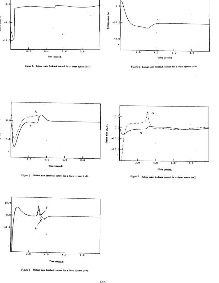
Figure 3 and Figure 4 show that we obtain accurate estimates of y and y in about 3.8 seconds. Figures 5 and 6 show that the system output y (=x ,) is regulated to "almost" zero, and x and x remain bounded.

5. Conclusions

In this paper, a new robust controller is proposed for uncertain linear systems. Given the knowledge of a nominal state space model as well as quantitative bounds on system uncertainties, the new controller achieves regulation of the system output and ensures boundedness of the system state. Unlike the Sliding Mode Controllers or the Ultimate Boundedness Controllers, the proposed controllers do not impose any structural conditions on the system uncertainties. However, the system is assumed to be minimum phase. When the relative degree of the system is larger than two, the proposed controller is first obtained

in an unrealizable form, and then its approximation in a realizable form is suggested. The robust controller in the approximated form is verified to be effective by a computer simulation study. In this paper we assume that the system state is directly accessible; however, we mention that a similar controller [8] has been developed for systems for which only a nominal transfer function is given and only the system output is measured.

References

G. Leitmann, "On the efficacy of nonlinear control in uncertain linear systems," J. Dynam. Syst., Meas. and Cont., vol. 103. no. E. P. Ryan and M. Corless, "Ultimate Boundedness and asymp- totical stability of a class of uncertain dynamical systems via con- tinuous and discontinuous feedback control," IMA Joumal of

Mathematical Control and Information, vol. 1, pp. 223-242, 1984. V. Utkin, "Variable Structure Systems with Sliding Modes,'' E E E Trans., Automat. Con@., vol. AC-22, pp. 212-222. 1977. B. Drazenovic, "The invariance conditions in variable structure systems," Automatica, vol. 5 , pp. 287-295, 1969.

2, pp. 95-102, 1981.

(4)

B. R. Barmish and G. Leitmann, "On ultimate boundedness control of uncertain systems in the absence of matching conditions," IEEE Trans., Automat. Contr., vol. AC-27. pp. 153-158, 1982.

J. S. Thorp and B. R. Barmish, "On guaranteed stability of uncertain linear systems via linear control," J. Optimiz. Theory and Appl., vol. 35, no. 4, pp. 559-579, 1981.

M. S . Chen and M. Tomizuka, "Disturbance Estimator and Its Application in Estimation of System Output Derivatives," Proceedings of the 28th IEEE Conference on Decision and Con- trol, Tampa, Florida, 1989.

M. S. Chen, Ph.D. Dissertation, On The Design of Nonlinear

Robust Controllers for Linear Sysrems, Department of Mechanical Engineering, University of California, Berkeley, 1989.

4 = .

Appendix A

Proof of Theorem 1: define V=% y 2 , and take the derivative of V: v = y y -

F

I

T

K =

-

zby2

-

-p(.r)yg(y)

+

y ( l - - ) C h

+

yG Ix

+

y d l K K

It follows from Assumptions (A4) and (A5) that

V ~ ~ K m ~ 2 - - m p ( ~ ) l y I g ( l y I ) + l y l h l c h l

+

l y l Q l l l x / l

+

I Y ~ D ? 0 1 0 . 0 0 0 1 . 0 0 0 0 . 1 . . ' '

t ; +

[Is

_03.7)

-&

-h,

-&

. - 5 - 2 where

Equation (A.1) shows that as long as ly I&,, the magnitude of y

decreases with a nonzero rate. Therefore, we conclude that y enters M I within a finite period of time, say T I (SV(O)l(oK,n ;)), and stays permanently inside M I after its first entry. It is clear from the definition of M I that n I can be made arbitrarily small if we choose sufficiently large p I , p, and p3. Since the system (1) is minimum phase and of relative degree one, we invoke Lemma 1 to conclude the boundedness of the system state x . This concludes the proof.

Appendix B

Proof of Theorem 2: a careful examination of Eq.(7) shows that the control input U is indeed a "normal" state feedback control. It then follows from Lemma 2 that

~ Z ~ - y ( ' ) i < E , i = I , . . . , r - I 03.1) within a finite period of time, and E, can be made arbitrarily small if

sufficiently large pI,'s and pn's in (2c) are used. Define another control input

u o = - g ( x ) + P ( x ) g ( s ) (B.2) K

where s is given by (4). and q ( x ) and p(x) are as defined by (7a). From the definitions of s and 3, and using (B.1). we have

3 = s

+

and I S k,-2Er-2+ ' +klE~ (B.3)

Consequently,

U = U'

+

p2p(x) and Ip2l 5 (0.4)

where

s

lies between s and 3. Notice that pI and p2 can be made arbitrarily small if f i ' s in (B.l) are all sufficiently small.

We now show that the control law (7) achieves regulation of the variable s. Define V=% s2, and take the derivative of V:

v = s s = s ( q ( . r ) + w u + G , x f d , ) = s ( q ( x ) + ~ u o + w C 1 ~ p ( x ) s x ~ ~ ) -

w

K K

where D O is an arbitrarily small number and

1

o h -

= I

I

I \

Y

(5)

I I I I

0.2 0 . 4 0.6 0.8

Tim (second,

-3.0-

F i W 1. Robust sue feedback wnml for I lincu cyrtem (r-I)

I I I

I I I I

4 . 0 6.0 8.0

2 . 0

Tim (second)

Figure 3 R&u iutc P e d W con001 for I linear system (-3)

I

lO.0C

Time (second)

Figure 4 Robu~ lute feedback cmml for I linear system (-3)