高階調變多輸入多輸出正交分頻多工系統中基於機率資料聯結演算法之資料檢測方法

國 立 交 通 大 學

電信工程學系

碩 士 論 文

高階調變多輸入多輸出正交分頻多工系統中

基於機率資料聯結演算法之資料檢測方法

Data Detection Methods Based on Probabilistic Data

Association Algorithm for High Order Modulation

MIMO-OFDM Systems

研究生：王冠群

指導教授：黃家齊 博士

高階調變多輸入多輸出正交分頻多工系統中

基於機率資料聯結演算法之資料檢測方法

Data Detection Methods Based on Probabilistic Data Association

Algorithms for High Order Modulation MIMO-OFDM Systems

研 究 生：王冠群 Student：Kuan-Chun Wang

指導教授：黃家齊 博士 Advisor：Dr. Chia-Chi Huang

國 立 交 通 大 學

電信工程學系

碩 士 論 文

A Thesis

Submitted to Department of Communication Engineering College of Electrical and Computer Engineering

National Chiao Tung University in partial Fulfillment of the Requirements

for the Degree of Master of Science

in

Communication Engineering June 2009

Hsinchu, Taiwan, Republic of China

高階調變多輸入多輸出正交分頻多工系統中

基於機率資料聯結演算法之資料檢測方法

學生：王冠群

指導教授：黃家齊博士

國立交通大學電信工程學系 碩士班

摘

要

今天我們的資訊社會的特點是變得越來越需要移動性以及無障礙性。

同時，對於高傳輸率的需求也大大的增加。多輸入多輸出正交分頻多工

(MIMO-OFDM)空間多工系統是一種可行的技術，它可以用來改進無線通訊

訊號的品質以及傳輸的速率。在 MIMO-OFDM 空間多工系統的資料檢測中，

球狀解碼是一種被廣泛使用的次佳解檢測器。它擁有非常好的效能，但是

它的複雜度會隨著通道和訊雜比而改變。在這篇論文中，我們證明了 SSIC

演 算 法 與 PDA 演 算 法 是 等 效 的 。 此 外 ， 我 們 提 出 了 兩 種 檢 測 器 ，

GPDA-MCPDA 與 GPDA-SD ， 用 來 降 低 球 狀 解 碼 在 接 近 最 佳 解 的

MIMO-OFDM 空間多工系統下使用高階 QAM 調變(16QAM/ 64QAM)的複

雜度。模擬結果顯示，這兩種檢測器都可以達到接近最佳解的效能而且它

們的優勢在於擁有比球狀解碼還低的複雜度，特別是在低訊雜比的區域。

Algorithms for High Order Modulation MIMO-OFDM System

Student：Kuan-Chun Wang

Advisors：Dr. Chia-Chi Huang

Department of

Communication Engineering

National Chiao Tung University

ABSTRACT

Our information society today is marked by an increasing need for mobility and accessibility. At the same time, the demand for ever higher data transfer rates is also increasing. A MIMO-OFDM spatial multiplexing system is a proven technology that can improve signal quality and data rate for wireless communications. Sphere Decoding (SD) algorithm is a popular suboptimal data detection method in a MIMO-OFDM spatial multiplexing system. It although performs very well but suffers from the fact that its complexity is a random variable depending on channel and signal to noise ratio (SNR). In this thesis, we establish the equivalence of the SSIC algorithm and the PDA algorithm. Furthermore, we proposed two detectors, GPDA-MCPDA and GPDA-SD, to reduce the complexity of the sphere decoding algorithm for near-optimal detection in a MIMO-OFDM spatial multiplexing system with higher order QAM constellations (16QAM/64QAM). Simulation results demonstrate that both detectors can achieve near-optimal performance with lower complexity as compare with the sphere decoding algorithm, especially at the low SNR regions.

首先感謝指導教授 黃家齊教授對於我研究及生活上的指導與勉勵，以

及對於論文內容的建議，使我得以順利完成碩士學位。同時也感謝 吳文榕

教授、 陳紹基教授以及 高銘盛教授給予本論文的指教，口試時也提供了

我許多的意見，使得論文更加完善。

特別感謝 古孟霖學長與 陸裕威學長，在我研究中所給予的指導，與學

長們的討論常使我獲益良多，使我的觀念更加地茁壯。感謝實驗室的同學，

奕廷、人豪、曉顗以及王森這兩年來的照顧與陪伴。感謝無線通訊實驗室

的所有成員與書含的陪伴，使我的生活充滿了歡樂與溫馨。

最後，感謝我的家人，給予我精神上的鼓勵與支持。特別要感謝姊姊，

在我寫論文的時候幫了我許多忙。

中文摘要 ... i 

ABSTRACT ... ii 

誌謝 ... iii 

Contents ... iv 

List of Tables ... vi 

List of Figures ... vii 

Chapter 1 Introduction ... 1 

Chapter 2 MIMO-OFDM System ... 4 

2.1 Overview of MIMO System ... 4 

2.2 Overview of OFDM System ... 5 

2.3 MIMO-OFDM System ... 5 

2.4 Detection Schemes on the Receiving Side ... 7 

Chapter 3 Probabilistic Data Association Based Detectors ... 9 

3.1 Probabilistic Data Association Detector ... 9 

3.1.1 Basic Algorithm ... 10 

3.1.2 Computational Refinements ... 13 

3.2 Generalized PDA Detector ... 14 

3.3 Simulation Results ... 16 

Chapter 4 Data Detection in MIMO-OFDM System Based on GPDA Detector ... 29 

4.1 GPDA-MCPDA Detector ... 29 

4.1.1 Markov Chain Monte Carlo Method ... 29 

4.1.1.1 Monte Carlo Integration ... 30 

4.1.1.2 Importance Sampling ... 31 

4.1.1.3 Introduction to Markov Chains ... 31 

4.1.1.4 Gibbs Sampler ... 35 

4.2.1.1 Real Sphere Decoding ... 42 

4.2.1.2 Complex Sphere Decoding ... 46 

4.2.2 GPDA-SD Detector ... 47 

4.3 Simulation Results ... 48 

Chapter 5 On the Equivalence between the SSIC Algorithm and the PDA Algorithm ... 61 

5.1 The SSIC Algorithm ... 61 

5.2 The Equivalence of the SSIC Algorithm and the PDA Algorithm ... 65 

5.3 Simulation Results ... 66 

Chapter 6 Conclusion ... 69 

Table 3.1 Simulation parameters for comparing PDA with GPDA. ... 17 Table 4.1 Simulation parameters for MIMO-OFDM system. ... 48 Table 5.1 Simulation parameters for SSIC algorithm and PDA algorithm. ... 66 

Fig. 2.1 MIMO-OFDM spatial multiplexing system. ... 6

Fig. 3.1 Block diagram of the basic PDA procedure. ... 12 

Fig. 3.2 The BER performance for PDA and GPDA with q=4. ... 20 

Fig. 3.3 The BER performance for PDA and GPDA with q=16. ... 21 

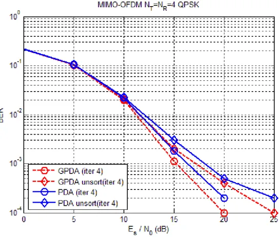
Fig. 3.4 The effect of sorting for PDA and GPDA with q=4. ... 22 

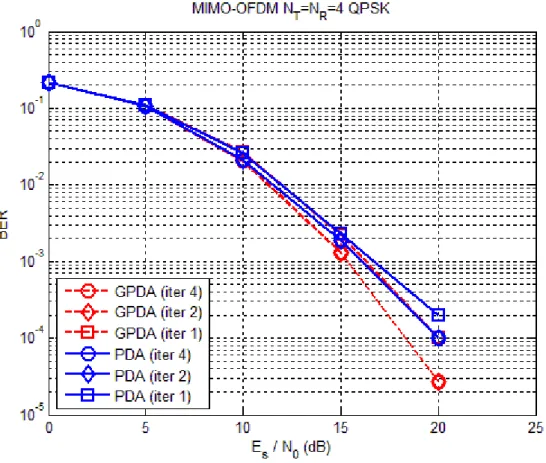
Fig. 3.5 The number of iterations for PDA and GPDA with q=4. ... 23 

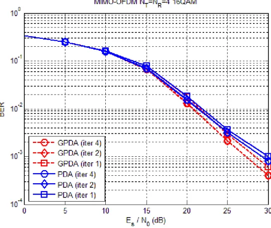
Fig. 3.6 The number of iterations for PDA and GPDA with q =16. ... 24 

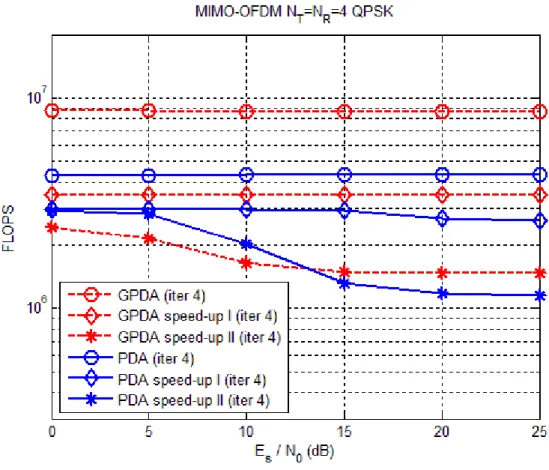
Fig. 3.7 The complexity for PDA and GPDA with q=4. ... 25 

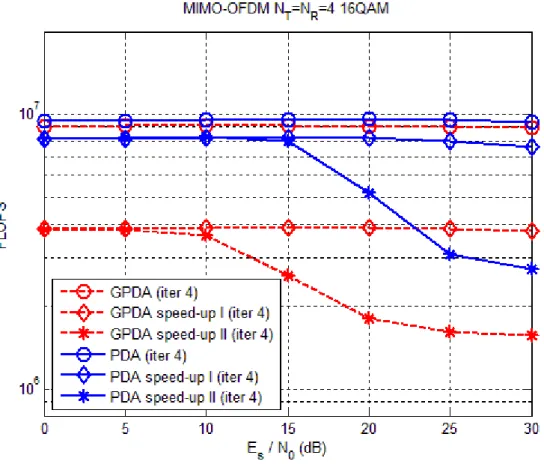
Fig. 3.8 The complexity for PDA and GPDA with q=16. ... 26 

Fig. 3.9 The complexity for PDA and GPDA with different modulation order. ... 27 

Fig. 3.10 The noise variance estimation error for GPDA and PDA. ... 28

Fig. 4.1 Block diagram of the GPDA-MCPDA detector. ... 40 

Fig. 4.2 The discrepancy between the PDA detector and the MCPDA detector. ... 41 

Fig. 4.3 A sphere of radius d and centered at

r

. ... 42 

Fig. 4.4 Search tree of sphere decoding... 44 

Fig. 4.5 Block diagram of the GPDA-SD detector. ... 48 

Fig. 4.6 The BER performance for MCMC detector with different initial point. ... 52 

Fig. 4.7 The BER performance for MCPDA detector with different initial point. ... 53 

Fig. 4.8 The BER performance for MCPDA detector with different iterations. ... 54 

Fig. 4.9 The BER performance for parallel MCPDA with different combinative iterations ... 55 

Fig. 4.10 The BER performance for different detection scheme with q=16. ... 56 

Fig. 4.11 The BER performance for different detection scheme with q=64. ... 57 

Fig. 4.12 The complexity for different detection scheme with q =16. ... 58 

Fig. 4.13 The complexity for different detection scheme with q=64. ... 59 

Fig. 4.14 The channel estimation error for different detection scheme. ... 60

Fig. 5.1 Block diagram of the basic SSIC procedure. ... 64 

Fig. 5.2 The BER performance for the SSIC algorithm and the PDA algorithm. ... 67 

Chapter 1

Introduction

The Multiple-input multiple-output orthogonal frequency division multiplexing (MIMO-OFDM) spatial multiplexing system [1] [2] is a proven technology that can improve signal quality and data rate for wireless communications. The global growth of interest in the wireless Internet and digitized audio and video, coupled with a growing wireless high-bandwidth infrastructure leads to a rapidly expanding market for wireless multimedia services. To cope with the growth, wireless services providers today are facing a number of challenges, which include the limited availability of the radio frequency spectrum and a complex time-varying wireless environment. In near future, wireless devices will have the features for always-available connection, higher data rate, longer distance, low-power consumption, better Quality of Service (QoS), fewer dropped packets, and higher network capacity in order to improve service quality for rapid service expansion and configurations. Combining OFDM with MIMO equipment is the most promising technology for delivering high data rates and robust performance.

In a MIMO-OFDM spatial multiplexing system, the optimum solution is to use Maximum Likelihood (ML) detection. However, ML detection is an exhaustive search; the complexity increases with either the increasing number of transmitting antennas or the

increasing order of modulation. Computational efficient data detection algorithms have been widely explored to achieve the substantial performance gains promised by MIMO-OFDM spatial multiplexing system with QAM constellations. There are two outstanding detectors of those frontrunners, the Sphere Decoding (SD) algorithm [3] and algorithm which based on the Probabilistic Data Association (PDA) [4] [5] principle. The SD algorithm although perform very well but suffers from the fact that its complexity is a random variable depending on channel and signal to noise ratio (SNR). The probabilistic data association is a simpler detection method, originally for Multi-User Detection (MUD) in synchronous Code Division Multiple Access (CDMA) [4]. The PDA based detectors perform well (close to the ML decoder) for simple modulation schemes i.e. BPSK and QPSK, but these results do not emerge from higher order modulations [5].

In this thesis, we focus on the higher order QAM constellations (16QAM/64QAM) data detection in the MIMO-OFDM spatial multiplexing system. We propose two near-optimal performance detectors with the common features which is using the Generalized PDA (GPDA) [5] detector at the low SNR regions. At the high SNR regions, we will combine different detectors to improve the performance. The first proposed detector is combining GPDA and Markov Chain Monte Carlo (MCMC) [6], and it is named MCPDA which incorporates the concept of PDA to calculate the covariance then construct a Markov Chain to make it converge to the target distribution. The second one is based on the SD algorithm using GPDA

solution to be the radius of the sphere. In addition, we prove the Soft Successive Interference Cancellation (SSIC) algorithm and the Probabilistic Data Association (PDA) algorithm are equivalent in the MIMO-OFDM system.

This thesis is organized as follows. In Chapter 2, we describe a MIMO-OFDM system. Chapter 3 introduces the PDA detector and the GPDA detector. In Chapter 4, we propose two modified methods (GPDA-MCPDA, GPDA-SD) of data detection in the MIMO-OFDM spatial multiplexing system. In Chapter 5, we establish the equivalence of the SSIC algorithm and the PDA algorithm in the MIMO-OFDM system. Finally, some conclusions are drawn in Chapter 6.

Chapter 2

MIMO-OFDM System

2.1 Overview of MIMO System

A MIMO system can be defined simply. Given an arbitrary wireless communication system, we consider a link for which the transmitting end as well as the receiving end is equipped with multiple antenna elements. The idea behind MIMO is that the signals on the transmit (TX) antennas at one end and the receive (RX) antennas at the other end are “combined” in such a way that the performance (bit-error rate or BER) or the data rate (bits/sec) of the communication for each MIMO user will be improved. Such an advantage can be used to increase both the network’s quality of service. One popular example of such a system is V-BLAST (Vertical-Bell Laboratories Layered Space-Time) suggested by Foschini et al [7].

MIMO techniques can be basically split into two groups: space time coding (STC) and spatial multiplexing (SM). STC increases the performance of the communication system by coding over the different transmitter branches; whereas SM achieves a higher throughput by transmitting independent data streams on the different transmit branches simultaneously at the same carrier frequency. Since increasing the bit rates is our goal, we will focus on the SM algorithms in this thesis. A potential application of the MIMO principle is the next-generation

wireless local area network (WLAN).

2.2 Overview of OFDM System

OFDM, which was brought up in the mid 60’s, is a digital multi-carrier modulation scheme. OFDM is used in numerous wireless transmission standards nowadays (DAB, DVB-T, WiMAX IEEE 802.16, ADSL, WLAN IEEE 802.11a/g), as a result of its capability of high-rate transmission and low-complexity implementation over frequency-selective fading channels.

The basic idea of OFDM is that it divides the available spectrum into several orthogonal subcarriers. Because these subcarriers are narrow-band, they experience flat fading channel and then equalization method of the system becomes very simple. Furthermore, it possesses high spectral efficiency by overlapping these orthogonal subcarriers [8]. Moreover, the insertions of the cyclic prefix (CP), which preserves the periodic extensions of the transmitted signal, can eliminate inter-symbol and inter-carrier interference caused by multipath environments.

2.3 MIMO-OFDM System

The combination of the throughput enhancement of MIMO with the robustness of OFDM against frequency-selective fading caused by severe multipath scattering and

narrowband interference is regarded as a very promising basis for future high data-rate radio communication systems. On the other hand, especially in multiplexing system, interference in MIMO-OFDM is severer than in single input single output (SISO) OFDM system and the complexity of data detection in a MIMO-OFDM system is higher than the complexity in SISO OFDM system.

  Fig. 2.1 MIMO-OFDM spatial multiplexing system.

In the MIMO-OFDM spatial multiplexing system, we consider the system shown in Fig. 2.1. We assume that there are transmitting antennas and receiving antennas. At the transmitter side, bit stream is divided into data layers and mapped each data layer to be

modulated signal streams. modulated signal streams in layer pass through

IFFT, add cyclic prefix and then transmit parallel through transmitting antennas. At the receiver side, there are receiving antennas. After cyclic prefix removal and FFT, the received signal vector can be expressed as

T N N R N T T N T N _T N_T N R N

r

= + r Ha v (2.1)

where is a by channel matrix, is a by 1 transmit vector of symbols, satisfying that each symbol in the constellation is transmitted with equal probability, and is an by 1 complex-valued white Gaussian noise vector with zero mean and covariance matrix equal to σ2I. By assuming a rich scattering model, the elements of the channel matrix

are independent and identically distributed (i.i.d.) complex Gaussian with zero mean.

H R N R N N_T

a

N_T

v

H

2.4 Detection Schemes on the Receiving Side

The complexity of the Maximum Likelihood (ML) detector grows exponentially with the number of transmitting antennas and the size of the signal constellation. This motivates the use of simpler suboptimum detectors in practical applications. Among those are:

„ Zero Forcing (ZF) detectors, which invert the channel matrix. The ZF receiver has a very small complexity that does not depend on the modulation. However, it does not completely exploit the system diversity and suffers from bad performance at low SNR.

„ Minimum Mean Square Error (MMSE) detectors, which reduce the combined effect of interference between the parallel channels and the additive noise. The MMSE receiver slightly improves the performance of the ZF receiver, but it requires knowledge of the SNR. Besides, it does not completely exploit the channel diversity either.

„ V-BLAST Ordered Successive Interference Cancellation (OSIC) [9], which exploits the timing synchronism inherent in the system model. Furthermore, linear nulling (i.e., ZF) or

MMSE is used to perform the detection. In other words, SIC is based on the subtraction of interference of already detected element of a from the received signal vector r. This results in a modified received vector in which effectively fewer interferers are present.

„ SD [3] algorithm, which reduces the number of symbol values used in the ML detector. Note that this type of detectors may preserve optimality while reducing implementation complexity.

Thus, if signal conditions are excellent, the data rate will be more than twice depending on the number of antennas used in both the transmitter and receiver. In that case, the channel matrix is better conditioned and the performance degradation of suboptimal detectors is reduced.

Chapter 3

Probabilistic Data Association Based Detectors

3.1 Probabilistic Data Association Detector

The Probabilistic Data Association (PDA) detector[4]is a highly successful approach to target tracking in the case that measurements are unlabeled and may be spurious. It is based on two approximations. Firstly, the PDA detector only looks at one transmitted symbol at a time, treating the received symbols as statistically independent. The second approximation is the Gaussian approximation (“Gaussian forcing”) of the probability density function (PDF) of the interference and noise. This is a bold and to some extent unjustifiable step, but it is difficult to argue with good performance and low complexity.

Now, to obtain the system model of the PDA detector, we multiply (2.1) form the left by

H

H

 

to obtain

=

+

y Ga n

(3.1)

where y H r= H , G H H= H , and n H v= H .

The model of the PDA detector is obtained by multiplying (3.1) from the left by G−1 to yield i i j j j i a a ≠ = + = +

∑

+ y a n e e n (3.2)

In (3.2), y G y= -1 , _{n G n}= -1 , and is a column vector whose ith element is 1 and the

i

other element are 0. In order to obtain computational efficiency, we choose (3.2) as the system model for the PDA algorithm.

3.1.1 Basic Algorithm

In the reformulated MIMO-OFDM spatial multiplexing system model (3.2), we treat the element of a as independent multivariate random variable where the ith element, , is a member of possible set:

i

a

{

( ) , 1,

}

[

]

i i i T

a ∈X = x m i∈ N (3.3)

In (3.3), is the set of distinct values of the QAM symbols. For any element , we associate a vector whose mth element,

i

X a_i

i

p p m_i( ), is the current estimate of the posterior that a_i =x_i(m). Since direct evaluation of Pr a

(

_i =x_i( )m y

)

is computationally prohibitive, the PDA algorithm attempts to estimate by using “Gaussian forcing” idea to approximate

(

)

Pr a_i = x m_i( ) y p,{ _j}_{∀ ≠j i} , which will serve as the update value for p m_i( ).

An important factor in the performance of the PDA algorithm is the order in which the probability vectors

{ }

p_{i ∀i} are updated. In this case, we use V-BLAST OSIC method [9] to order the update sequence according to SNR in descending order, which can detect the first signal that belongs to the highest order of SNR. It is useful to provide the reliable symbols from the high SNR, and we can use these reliable symbols to detect the other symbols to make the BER performance better.

To estimate the associated probabilities for an element , we treat all other elements as multivariate random variables, and from (3.2), we define

i a ( j a j i≠ ) i j j j i a ≠ =

∑

+ N e n i (3.4)

as the effective noise on , and approximate it as a Gaussian noise with matched mean and covariance: a [ ] i j j i j E a ≠ =

∑

N e (3.5) 2 -1 [ ] T i j j j j i Var a σ ≠ =

∑

+ Ω e e G (3.6)

where N_i =E[N ]_i and Ω_i =Cov[N_i]. In (3.5) and (3.6), E[a and Var[ ]_j] a are given by _j E[ _j] _j( ) _j( ) m a =

∑

x m p m _(3.7) 2 2 Var[ _j] _j( ) _j( ) (E[ _j]) m a =

∑

x m p m − a _(3.8) Therefore, we can calculate P

(

y a_i =x m_i( )

)

as follows:

_{( ( )) exp}

(

_{( ( ) )}H 1_{( ( )}

)

i i i i i i i i i P ya =x m ∝ − −y ex m −N Ω y e− − x m −N ) (3.9) Then, we let i = − i θ y N       (3.10) and 1 1 1 1 1 ( ) ( ( ) ) ( ( ) (2 ( ) 2 ) ( ) (2 ( )) ( ) [2 ] [ ] ( )[ ] ( ) H i i i i i i i i H i i i i i i H i i i i i i H H i j i ji i i ii i j m x m x m x m x m x m x m ) x m x α − − − − − = − − − − − ∝ − − = − ⎛ ⎞ =_⎜ − _⎟ ⎝

∑

⎠ y e N Ω y e N y e N Ω e θ e Ω e θ Ω Ω m       (3.11)

where [2θ_iH]_j is the jth element of 2θ ; _iH [Ω_i−1]_ji is the element (j,i) of i1. The posterior

− Ω

probability P m_i( ) is then given as exp( ( )) ( ) exp( ( )) i i i l m P m l α α =

∑

(3.12) , ( ) 1 1 i i i P m X Initialize iter ⎧∀ = ⎨ ₌ ⎩ 1 Initialize i= ( ) i Calculate P m T

i N

<

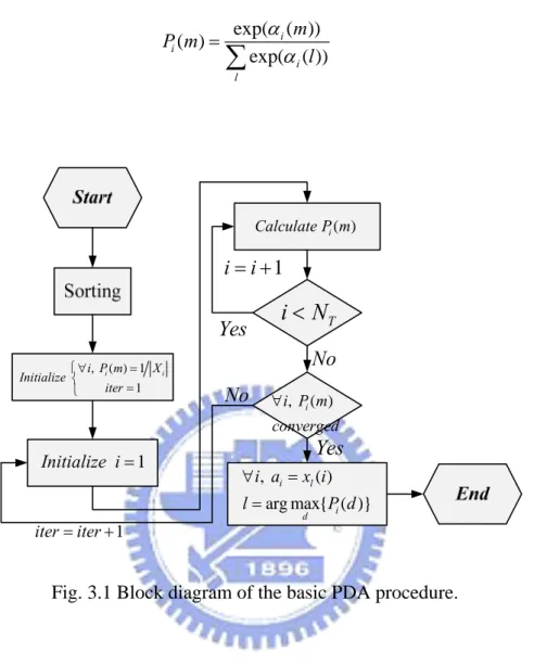
1 i i= + No , ( ) i i P m converged ∀ , ( ) arg max{ ( )} i l i d i a x i l P d ∀ = = Yes No Yes 1 iter iter= +

Fig. 3.1 Block diagram of the basic PDA procedure.

The basic procedure for the PDA detector is as follows:

1. Based on the matrix in (3.1), we obtain the optimal detection sequence proposed for the V-BLAST OSIC in [9]and denote the sequence as

G

1

{ }NT

i i

k ₌ .

2. Initialize the probabilities as P m_i( ) 1= X_i ,∀ ∀ , and set the iteration counter m i iter=1. 3. Initialize i = 1.

4. Based on the current values of {p_kj}_kj≠ki , we use the “Gaussian forcing” idea to approximate Pr

(

( ) ,{

)

i i

k k

a =x m y p } ∀m

j j i

corresponding elements of .

i

k

p

5. If i N< _T , let i= +i 1 and back to step 4. Otherwise, carry on step 6.

6. If ∀i, p_i has converged, go to step 7. Otherwise, let iter=iter+1 and return to step 3. 7. For j=1,...,N_T, make a decision ˆa for _j a via _j

ˆ_{j j}( ), arg max{ _j( )}

m

a = x l l= p m (3.13)

The block diagram of the basic PDA procedure is shown in Fig. 3.1.

3.1.2 Computational Refinements

A. Speed-Up–Matrix arithmetic

As noted in [4], although the computation in step 4 is no longer exponential, to calculate the inverse of for each element directly is still expensive. Further simplifications can be evaluated by applying the Sherman-Morrison-Woodbury formula [10] twice consecutively.

i

Ω

1. Define auxiliary variables Ω

[ ] (3.14) T i i iVar ai = + Ω Ω e e 2. Compute Ω_i−1 via 1 1 1 1 1 [ ] 1 [ T i i i ] T i i i Var a Var a − − − − − = + + Ω e e Ω Ω Ω e Ω e (3.15) i

3. Compute P m_i( ) and update E a[ ]_i , Var[ ]a_i . 4. Compute Ω−1 via

1 1 1 1 1 [ ] 1 [ T i i i i i i T i i i i Var a Var a − − − − − = − + Ω e e Ω Ω Ω e Ω e ]

a

V (3.16) B. Speed-Up–Successive Skip

In our simulations, we have observed that the algorithm generally converges within 2 to 4 iterations for SNR < 14 dB, and within 1 to 2 iterations for SNR > 14 dB. However, the overall complexity can be high if one or two elements of exhibit slow convergence. To reduce the complexity in these instances, successive skip is applied each iteration. Note that, the successive skip method is different from the successive cancellation method which mentioned in [4]. The advantage of the successive skip method is implemented easily and lower complexity than the successive cancellation method. The main idea of the successive skip tactic is that the posterior probability of some elements is high enough to let us believe it within the process of converges. So, if we have this element in the next iteration, we can simply skip it.

After zth iteration, we define to be the set of elements that satisfy

max{ ( )} )P m_{i ∀m} ≥ ∀

ε

, i (3.17)

where

ε

= −1 (0.2

σ

2) is a small positive number. At z+1th iteration, we will skip the elements that belong to V .

3.2 Generalized PDA Detector

square/rectangular (sqr/rect) QAM. In the case of sqr/rect q-QAM, the GPDA algorithm differs from the PDA approach of [11] by reducing the number of probabilities associated with each transmit symbol. As an apparent consequence of reducing the number of probabilities for sqr/rect QAM, the GPDA shows an improved error probability over the PDA approach used in [11]. A further advantage of GPDA is that it offers a reduced computational cost over that of [11] for the case when the number of receive antennas is greater than the number of transmit antennas.

To obtain the system model for sqr/rect QAM version of the GPDA detector, we begin by transforming (2.1) into the real-valued vector equation

= + r Ha v (3.18) where

{ } { }

{ } { }

{ } { }

{ }

{ }

{ }

{ }

T T T T T T T T T ⎡ ⎤ = ℜ_⎣ ℑ _⎦ ⎡ ⎤ = ℜ_⎣ ℑ _⎦ ⎡ ⎤ = ℜ_⎣ ℑ _⎦ ℜ −ℑ ⎡ ⎤ = ⎢_{ℑ ℜ} ⎥ ⎣ ⎦ r r r a a a v v v H H H H H (3.19)

Next we multiply (3.18) from the left by HT to obtain = +

y Ga n (3.20)

where y H r= T , , and . Note that, because the element of are modeled as i.i.d. complex Gaussian, will almost always have full rank and consequently the symmetric matrix will be positive definite with probability nearly one.

T = G H H _{n H v=} T H H G

The model for sqrt/rect QAM version of the GPDA detector is obtained by multiplying (3.20) from the left by _G−1 to yield

i i j j j i a a ≠ = + = +

∑

+ y a n e e n (3.21)

In (3.21), y G y= -1 , , and is a column vector whose ith element is 1 and whose other element are 0. is a member of one of two possible sets:

-1 = n G n i a i e { ( )}, [1, ] { ( )}, [ 1, 2 ] i i T i i i T T S X x m i N a S X x m i N N ℜ ℑ = = ∈ ⎧ ∈ ⎨ _{= = ∈ +} ⎩ (3.22)

In (3.22), and S are the sets of distinct values that can be assumed by the real and imaginary parts of the QAM symbols respectively. Thus equation (3.21) can be solved via PDA which we introduced in Section 3.1. Note that, when we calculate equation (3.9) in the GPDA algorithm, it should be modeling by the real Gaussian distribution rather than the complex Gaussian distribution and the noise variance should be

S_{ℜ ℑ}

2 2

σ

rather than σ . 2

3.3 Simulation Results

Perfect Channel State Information (CSI) Perfect noise variance estimation

Number of subcarrier 64 Length of cyclic prefix 16

Channel Rayleigh Fading

Relative power (dB) (0,0)

Modulation QPSK, 16QAM, 64QAM

Table 3.1 Simulation parameters for comparing PDA with GPDA.

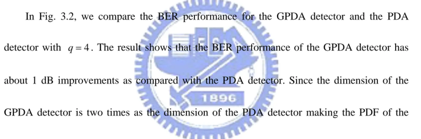
In this Section, we use several computer simulation examples to show the performance and the computational cost of the PDA detector and the GPDA detector. We also compare the PDA detector and the GPDA detector with the V-BLAST ZF OSIC [9] and the optimal ML detector in the examples. The simulation parameters are shown in Table 3.1.

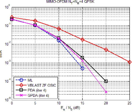
In Fig. 3.2, we compare the BER performance for the GPDA detector and the PDA detector with . The result shows that the BER performance of the GPDA detector has about 1 dB improvements as compared with the PDA detector. Since the dimension of the GPDA detector is two times as the dimension of the PDA detector making the PDF of the interference and noise closer to Gaussian distribution. In Fig. 3.3, it shows the performance of the aforementioned detectors for the case

4

q=

16

q= .

In Fig. 3.4, we compare the effect of sorting for the GPDA detector and the PDA detector with . The result shows that the BER performance of the PDA and the GPDA detectors has approximately more 2 dB than that of the unsorted PDA and the unsorted GPDA detectors. Thus, we can identify that sorting is an important factor for the GPDA and the PDA detectors.

4

q=

detector with . The result shows that both the GPDA detector and the PDA detector just need 2-4 iterations to converge. In Fig. 3.6, it shows the BER performance of the aforementioned detectors for the case

4

q=

16

q = .

In Fig. 3.7, we compare the complexity for the GPDA detector and the PDA detector with . For the case of complexity of the system, the measurement was calculated using FLOPS function in MATLAB [14], which counts the approximated floating point operations that the algorithm needs to complete decoding in one block of transmitted symbols. The result shows that there is a great gap of the original complexity between the GPDA detector and the PDA detector. After using the matrix speed-up (speed-up I) tactic, the gap between the GPDA detector and the PDA detector has reduced. If we use matrix speed-up tactic and successive skip tactic simultaneously (speed-up II), the complexity may reduce once more. Overall, the complexity of the GPDA detector is slight more than that of the PDA detector for

4

q=

4

q= . In Fig. 3.8, we compare the complexity for the GPDA detector and the PDA detector with . As the figure suggests that, after using speed-up tactic, the complexity of the GPDA detector will be significantly less than that of the PDA detector.

16

q=

In Fig. 3.9, we compare the complexity for the GPDA detector and the PDA detector with different modulation order, at SNR=0 dB. We can observe that with greater modulation order, the gap between the GPDA detector and the PDA detector gets wider.

detector with , at SNR=25 dB. The result shows that the GPDA detector and the PDA detector are almost free from the impact of the noise variance estimated error. Note that,

16 q = [ E 2 2 [ ] [ ] E E 2 ]

σ

=

σ

+ Δ

σ

where E[ ]

σ

2 is estimated noise variance composed of real noise

variance E[

σ

2] and estimation error E[Δ

σ

2].

After above comparisons, the GPDA detector shows improved BER performance over the PDA detector by reducing the number of probabilities associated with each transmit symbol. Moreover, the complexity of the GPDA detector is much less than that of the PDA detector, especially in high order modulation. Hence, that is the reason why we choose the GPDA detector rather than the PDA detector.

Chapter 4

Data Detection in MIMO-OFDM System Based on

GPDA Detector

4.1 GPDA-MCPDA Detector

The basic idea of the GPDA-MCPDA detector is using the GPDA detector at the low SNR regions, and using parallel MCPDA method to generate numbers of random samples at the high SNR regions. After generating samples, we will pick up a sample from the final iteration of parallels, and the sample which has minimum distance (i.e. 2

arg min

i

a X∈ r - Ha ).

Thus, we can get a solution from the GPDA-MCPDA detector.

4.1.1

Markov Chain Monte Carlo Method

A major limitation towards more widespread implementation of Bayesian approaches is that obtaining the posterior distribution often requires the integration of high-dimensional functions. This can be computationally very difficult, but several approaches short of direct integration have been proposed. The MCMC methods [6], which attempt to simulate direct draws from some complex distribution of interest. MCMC approaches are so-named because one uses the previous to randomly generate the next sample value, generating a Markov Chain (as the transition probabilities between sample values are only a function of the most recent

sample value).

The realization in the early 1990’s that one particular MCMC method, the Gibbs sampler, is widely applied to a broad class of Bayesian problems has sparked a major increase in the application of Bayesian analysis.

4.1.1.1

Monte Carlo Integration

The original Monte Carlo approach was a method developed by physicists to use random number generation to compute integrals. Suppose we wish to compute a complex integral

( )

b ah x dx

∫

(4.1)

If we can decompose h x( ) into the production of a function f x( ) and a probability density function p x( ) defined over the interval (a,b), then note that

( ) ( ) ( ) ( ) [ ( )] b b p x a h x dx= a f x p x dx E= f x

∫

∫

(4.2)

so that the integral can be expressed as an expectation of f x( ) over the density p x( ). Thus, if we draw a large number x₁, ,x_n of random variables from the density p x( ), then

( ) 1 1 ( ) [ ( )] ( ) n b p x a i h x dx E f x f x n = =

∑

∫

i (4.3)

This is referred to as Monte Carlo integration.

Monte Carlo integration can be used to approximate posterior (or marginal posterior) distributions required for a Bayesian analysis. Consider the integral ( )I y =

∫

f y x p x d( | ) ( ) x , which we approximate by

1 1 ˆ( ) ( | ) n i i I y f y x n = =

∑

(4.4)

where x_i are draws from the density p x( ).

4.1.1.2

Importance Sampling

It was observed in the preceding Section 4.1.1.1 that the integral can be approximate by Monte Carlo integration. However, not every density p x( ) can be drawn directly. Now, we suppose the density q x( ) roughly approximates the density p x( ), then

( ) ( ) ( ) ( ) ( ) ( )( ) ( ) [ ( )( )] ( ) q x ( ) p x p f x p x dx f x q x dx E f x q x q x = =

∫

∫

x (4.5)

This forms the basis for the method of importance sampling, with

1 ( ) 1 ( ) ( ) ( ) ( ) n i i i i p x f x p x dx f x n

∑

= q

∫

_x (4.6) where x_i are draws from the density q x( ).

4.1.1.3

Introduction to Markov Chains

Before introducing the Gibbs sampler, a few introductory comments on Markov Chains are in order. Let denote the value of a random variable at time , and let the state space refer to the range of possible

t

X t

X values. The random variable is a Markov process if the transition probabilities between different values in the state space depend only on the random variable’s current state, i.e.,

1 0 1

Pr(X_t+ =s X_j| =s_k, ,X_t =s_i)=Pr(X_t+ =s X_j| _t =s_i) (4.7) Thus for a Markov random variable the only information about the past needed to predict the future is the current stage of the random variable, knowledge of the values of earlier states do not change the transition probability. A Markov chain refers to a sequence of random variables generated by a Markov process. A particular chain is defined most critically by its transition probabilities,

0

(X , X_n)

( , ) ( )

p i j = p i→ j , which is the probability that a process at stage s_i moves to state s in a single step, _j

1 ( , ) ( ) Pr( _{t j}| _t ) p i j = p i→ =j X + =s X =si (4.8) Let ( ) Pr( ) j t Xt sj π = = (4.9)

denote the probability that the chain is in state j at time , and let denote the row vector of the state space probabilities at step . We start the chain by specifying a starting vector . Often all the elements of are zero except for a single element of 1, corresponding to the process starting in that particular state. As the chain progresses, the probability values get spread out over the possible state space.

t

π

( )

t

t

)

(0)

π

π

(0

The probability that the chain has state value s_i at time (or step) is given by the Chapman-Kolomogrov equation, which sum over the probability of being in a particular state at the current step and the transition probability from that state into state

1

t+

i

1 1 ( 1) Pr( ) Pr( | ) Pr( ) Pr( ) ( ) Pr( , ) ( ) i t i t i t k t k k k k k k t X s X s X s X s k i t k i t π π π + + + = = = = = = → =

∑

∑

∑

= (4.10)

Successive iteration of the Chapman-Kolomogrov equation describes the evolution of the chain.

We can more compactly write the Chapman-Kolomogrov equation in matrix form as follows. Define the probability transition matrix P as the matrix whose i j, th element is

( , )

P i j , the probability of moving from state to state i j , P i( → j) . The Chapman-Kolomogrov equation becomes

( 1)

t

+ =

( )

t

π

π P

(4.11)

Using the matrix form, we immediately see how to quickly iterate the Chapman-Kolomogrov equation, as

2 ( )t = (t−1) =( (t−2) ) = (t−2)

π π P π P P π P (4.12) Continuing in this fashion show that

( )t = (0) t

π π P (4.13) Defining the n-step transition probability p as the probability that the process is in state _{i j}( )_,n

j given that it started in state , n step ago, i.e., i

( )

, Pr( | )

n

i j t n j t i

p = X₊ =s X =s (4.14) it immediately follows that p is just the i,j-th element of _{i j}n_, Pn.

( )

, 0

n i j

p > for all . That is, all states communicate with each other, as one can always go

from any state to any other state (although it may take more than one step). Likewise, a chain is said to be aperiodic when the number of steps required to move between two states (say

,

i j

x

and ) is not required to be multiple of some integer. Put another way, the chain is not forced into some cycle of fixed length between certain states.

y

*

π

* *

A Markov chain may reach a stationary distribution , where the vector of probabilities of being in any particular given state is independent of the initial condition. The stationary distribution satisfies

=

π π P

*

(4.15) The condition for a stationary distribution is that the chain is irreducible and aperiodic. When a chain is periodic, it can cycle in a deterministic fashion between states and hence never settles down to a stationary distribution.

A sufficient condition for a unique stationary distribution is that the detailed balance equation holds,

*

( ) _j ( ) _k

P j→k π =P k→ j π (4.16)

If equation (4.16) holds for all , the Markov chain is said to be reversible, and hence equation (4.16) is also called the reversibility condition. Note that this condition implies

, as the

,

i k

= π πP jth element of πP is ( )_{j i} ( ) _j ( ) _j ( ) i i i P i j P j i P j i _i π π π =

∑

→ =

∑

→ =

∑

→ πP =π (4.17)

with the last step following since rows sum to one.

4.1.1.4

Gibbs Sampler

One problem with applying Monte Carlo integration is in obtaining samples from some complex probability distribution. Attempts to solve this problem are the roots of MCMC methods. In particular, they trace to attempts by mathematical physicists to integrate very complex functions by random sampling, and resulting Metropolis-Hastings sampling [6]. The Gibbs sampler [6] [15] (introduced in the context of image processing by Geman 1984), is a special case of Metropolis-Hastings sampling wherein the random value is always accepted (i.e. α =1). The task remains to specify how to construct a Markov Chain with values converged to the target distribution. The key to the Gibbs sampler is that we only consider the univariate conditional distributions (the distribution when all of the random variables but one is assigned fixed value). Such conditional distributions are far easier to simulate than complex joint distributions and usually have simpler forms. Thus, we simulate n random variables sequentially from the n univariate conditions rather than generating a single n-dimensional vector in a single pass using the full joint distribution.

To introduce the Gibbs sampler, consider a bivariate random variable ( , )x y , and suppose we want to compute one or both marginal, p x( ) and p y( ). The idea behind the sampler is that it is far easier to consider a sequence of conditional distributions, p x y( | ) and

( | )

p y x , than to obtain the marginal by integral of the joint density p x y( , ), e.g.,

( ) ( , )

p x =

∫

p x y dy. The sampler starts with some initial value y₀ for y and obtains x₀ by generating a random variable from the conditional distribution, p x y( | = y₀). We use x₀ to generate a new value of from the sampler. To do so, we draw from the conditional distribution based on the value

1 y

0

x , p y x x( | = ₀). The sampler proceeds as follows: ~ ( | i i 1) x p x y y= ₋ (4.18) ~ ( | i y p y x x= _i) (4.19)

Repeating this process for k times, then it generates a Gibbs sequence of length k, where a subset of points ( ,x y for _{j j}) 1≤ ≤j m k< is taken as our simulated draws from the full joint distribution. The first m times of the process, called burn-in period, can make the Markov Chain converge to the distribution that near its stationary one.

When more than two variables are involved, the sampler is extended in the obvious fashion. In particular, the value of the kth variable is drawn from the distribution

where denotes a vector containing all of the variables but k. Thus, during the ith iteration of the sample, to obtain the value of _i( )k

( ) ( k | p

θ

( ) ) k − θ _θ( k− )

θ , we draw fro the distribution

, k+

_θ

n = m ( ) , i ( ) ( ) 1) ( 1) ( ~ ( , k k k k i p

θ

θ

θ

−

θ

−

θ

+ − − (1) | (1) i i ( 1) ( , , k

θ

θ

= = les, ( , , ,w x ( 1)

θ

) 1 1) n

θ

= i (4.20)

For example, if there are four variab y z) | ~ ( | ~ ( | i i x x x p x w w y p y w w

, the sampler beco

i i m i es 1 1 , , , , , ~ ( | , , ) i i i i i i i y y z x x z z z p z w w x x y y 1 1 ~ ( , ) i i i i w p w = y y z z 1 1) ) z − = − = − − − − = = = = = = = = = (4.21)

Now, we consider the equation (3.2) and we use Gibbs sampler to generate samples of from the distribution

a

( | )

P a y . The procedure as follows:

b T T T T N b s n n n-1 2 2 1 3 for n N 1 to N ple a from (P a a a| , , = − + i n n-1 n-1 n-1 1 1 2 3 N n-1 N n n N N 1

generate initial samples randomly

sample from ( | , , , , ) sam , , ) sample from ( | a P a a a a a a P a a − a y y i T n n 2 N 1 , , , , ) end a a ₋ y

then, we consider P a( _i|a y , and it can be factorize as ₋n_i, )

n n n n n n ( _i) ( P y a₋ P an n n n n n n n n n ( , ) ( ) ( , ) ( , ) ( , ) ( ) ( ) ) ( , ) ( ) ( ) ( , ) ( ) ( , ) ( ) ( , ) ( , ) i i i i i i i i i i i i i i i i i i i i i i i i i i i a i i i i a P a P a P a P P a P a P a P a P a P P a P a P a P a P a P a − − − − − − − − − − − − − − − = = = = =

∑

∑

y a a y y a y a a y a a y a y a a y a a y a y a       (4.22) where T n n n n-1 n 1 1 1 [ , , , , , i a a ai i a − = − + a … … -1 N ] and n ( _{i i}( ), _i

P ya =x m a₋) can be calculated as follows:

T T N -1 n n 1 1 N -1 n n 1 1 n 1 1 ( ( ), ) exp( ( ( ) ) ( ) i H i i i i i j j j j j j i i i i j j j P a x m x m a a x m a − − − = = + − = = 1 ( _{j j} )) j i a = + ∝ − − − − Φ −

∑

∑

∑

∑

y a y e e e e (4.23) thus, we define − − y e e

( ) i m

γ

T T T N N -1 -1 n n 1 1 n n 1 1 1 1 N -1 1 n 1 1 1 1 n 1 ( ( ) ) ( ( ) )) (2 ( ) 2 ) ( ) Let (2 ( )) ( ) i i H i i j j j j i i j j j j j j i j j i i H i i i i i i j j j j j j i H i i i i i x m a a x m a a x m x m a a x m x m − − − = = + = = + − − = = + − = − − − − Φ − − − ⎛ ⎞ ∝ − − Λ Φ _⎜ Λ = − _⎟ ⎝ ⎠ = − Φ

∑

∑

∑

∑

∑

∑

y e e e y e e e y e e e e κ e e

(

)

1 1 Let [2 ] [ ] ( )[ ] ( ) i i H H i j ji i ii i j x m x m − − = −Λ ⎛ ⎞ =_⎜ Φ − Φ _⎟ ⎝

∑

⎠ κ y κ (4.24)

where [2κ_iH]_j is the jth element of 2κ , H_i 1

[Φ− ]_ji is the element (j,i) of Φ−1 and

2

σ −1

Φ = G _(4.25)

finally, we can obtain

n n ( , ) ( , ) exp( ( )) i i i i i l P a P a l

γ

− − =

∑

y a a y (4.26)

In this routine, “for” loop examines the state variables a_k in order, N_b+N_s times. The first N_b iterations of the loop, called burn-in period, are to let the Markov Chain converge to near its stationary distribution. During the next N_s iterations, the Gibbs sampler generate the N_s samples, i.e.,

T n n n n 1, 2, N T a a , a ⎡ ⎤ = ⎣ ⎦

a , for n 1, 2,= , N_s. In general, the

t sample can be istribution should be converged

after

las the solution of the distribution. Since the d

b s

N +N times iteration.

There are two problems of Gibbs sampler:

1) How do you choose an initial point? A poor choice of initial point will greatly increase the required burn-in time, and an area of much current research is whether an optimal initial point can be found.

2) How many iterates are needed? This question does not have exact answer, the majority

.1.2 GPDA-MCPDA Detector

at higher values of SNR, some of the transition

tioned answers are obtained from the experience.

4

In [12], the author mentioned that

probabilities in the underlying Markov Chain may become very small. As a result, the Markov Chain may be effectively divided into a number of nearly disjoint chains. The term nearly disjoint here means the transition probabilities that allow movement between the disjoint chains are very low. Therefore, a Gibbs sampler that starts from a random point will remain within the set of points surrounding the initial point and thus may not get a chance of visiting sufficient points to find the global solution. In [13] two solutions for solving this problem were proposed: (i) run a number of parallel Gibbs sampler with different initial points; (ii) while running the Gibbs sampler, we assume a noise variance which is higher than it actually is. These two methods turned out to be effective for low and medium SNRs.

In the parallel MCPDA detector, we will focus on these two methods which men

above to improve the performance of MCMC method. First, we use parallel Gibbs samplers with the initial point generated randomly. Second, we compute covariance according to (3.6) rather than (4.25), so named MCPDA. Since we take the variance of residual interference caused by the random samples into account in the equation (3.6), the covariance will increase.

Furthermore, with few times of iteration, the covariance will be gradually narrowing. This may be regarded as automatic Simulated Annealing method [6]. Finally, we will pick up a sample from the final iteration of parallels, and the sample which has minimum distance (i.e.

2

arg min

i

a X∈ r - Ha ). Thus, we can get a solution from the parallel MCPDA detector.

r 3, we have mentioned that the GPDA detector performs well at th

In Chapte e low SNR

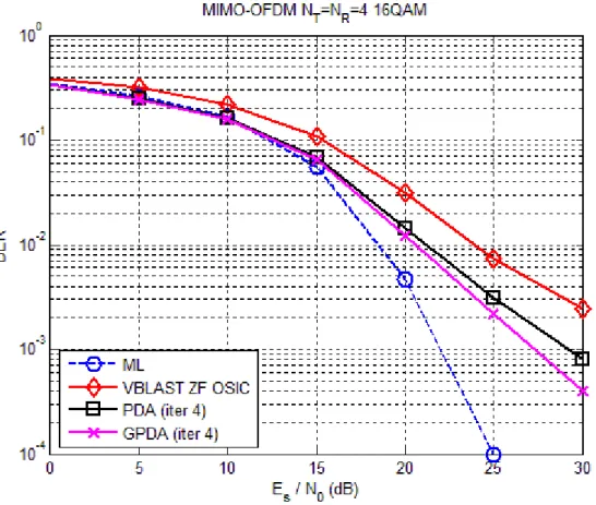
regions, so we can only use the GPDA detector at the low SNR regions; however, with the SNR increasing (exceed M dB), the performance of the GPDA detector will get worse gradually. Thus, we need to use parallel MCPDA method to assist the GPDA detector in order to reach better performance, so named GPDA-MCPDA detector. Moreover, MCPDA is similar to GPDA, we only need to add few blocks, and then the GPDA detector will become the MCPDA detector. Therefore, it may be quite simple to implement. The block diagram of the GPDA-MCPDA detector is shown in Fig. 4.1 and the discrepancy between the GPDA detector and the MCPDA detector is shown in Fig. 4.2.

1 − Ω ˆ GPDA X _ 2 ˆ Rand X _ ˆ Rand M X 2 ˆ arg min r - Hx _1 ˆ Rand X ˆ a 2 , ,σ r H 2 , ,σ r H

, ( ) 1 1 i i i P m X Initialize iter ⎧∀ = ⎨ ₌ ⎩ Start Sorting 1 Initialize i= ( ) i Calculate P m T i N< 1 i i= + No , ( ) i i P m converged ∀ Yes No End 1 iter iter= + Yes PDA MCPDA Draw sample Calculate by (3.6) and (4.26) Generate initial sample s N ˆ= a a

Fig. 4.2 The discrepancy between the PDA detector and the MCPDA detector.  

.2 GPDA-SD Detector

not have good performance at the high SNR

.2.1 Sphere Decoding

e lgorithm is a quasi-ML detection technique. It promises to find

4

As we know, the GPDA detector does

regions. In order to solve this problem, we try to find a solution which is better than the GPDA solution. Therefore, we use the Sphere Decoding (SD) algorithm to do this work, so named GPDA-SD, which can attain a better performance and lower complexity in the MIMO-OFDM spatial multiplexing system.

4

Th sphere decoding [3] a

was first introduced by Finke and Pohst [16] in the context of the closest point search in lattices but it has become very popular in digital communication literature. Its various applications include lattice codes, CDMA systems, MIMO systems, global positioning system (GPS), etc.

4.2.1.1 Real Sphere Decoding

Fig. 4.3 A sphere of radius and centered at

In communication system, the SD algorithm is used to solve the ML problem as follows:

d

r

. 2 ML ˆ arg min i a X∈ = a _{r - Ha (4.27)}

The computational complexity of above exhaustive search

m

method is really high. Therefore, the SD algorithm is brought up to avoid the exhaustive search and search only over the possible a which lie in a certain sphere of radius d around the given vector

r

, thereby reducing the search space and, hence, the required co putations (see Fig. 4.3).

It is clear that the closest point inside the sphere will also be the closest point for the who

ny points,

2) oints are inside the sphere? If this requires testing the distance of

The SD algorithm does not really address the first question, but usually uses ZF solution to be le point. However, close scrutiny of this basic ideal leads to two key questions.

1) How do you choose radius d? Clearly, if radius is too large, we obtain too ma

and the search remains exponential in size, whereas if radius is too small, we obtain no points inside the sphere.

How can we tell which p

each point form

r

, then there is no point in SD, as we will still need an exhaustive search.

the radius of the sphere. However it does propose an efficient way to answer the second. The basic observation is the following. Although it is difficult to determine the points inside a general N_T-dimensional sphere, it is trivial to do so in the one-dimensional case. The reason is that a one dimensional sphere reduces to the endpoints of an interval, and so the desired points will be the integer values that lie in this interval. We can use this observation to go from dimension k to dimension k +1. Suppose that we have determined allk-dimensional

points that lie in sphere of radius Then, for any such k -dimensional point, the set of admissible values of the

(

k

+

1)

th d ensional coordinate th lie in the higher dimensional sphere of the same radius ms an interval.

The above means that we can determine all

a d.

im at

d for

radius d by successively determining all points in spheres of lower dimensions 1, , N_T and the same radius d . Such an algorithm for determining the points in an N_T-di

sphere essentially constructs a tree where the branches in the kth level of the tree correspond to the points inside the sphere of radius d and dimension k (see Fig. 4.4). Moreover, the complexity of such an algorithm will depend on the size of the tree, i.e., on the number of points visited by the algorithm in different dimensions.

2,

mensional

at hand. To this Fig. 4.4 Search tree of sphere decoding.

With this brief discussion, we can now be mo e specific about the problemr

end, we shall assume that

N

_R

≥

N

_T. Note that, the point Ha lies inside a sphere of radius

d centered at

r

if and only if

2 2

d ≥ r - Ha _(4.28)

In order to break the problem into the sub-problems described above, it is useful to consider the QR factorization of the matrix H

R T T ( N N ) N 0 _{− ×} ⎡ ⎤ ⎢ ⎥ ⎣ ⎦ R Q = H _(4.29)

where R is N_T by N_T upper triangular matrix, and Q Q Q=[ _{1 2}] is an N_R by N_R N orthogonal matrix. The matrices Q₁ and Q₂ represent the first N_T and last N_R− _T orthonormal columns of Q, respectively. The condition (4.28) can be written as

2 2 [ ] d _{1 2} 2 1 2 2 2 1 2 0 0 H H H H ⎡ ⎤ ≥ − _{⎢ ⎥} ⎣ ⎦ ⎡ ⎤ ⎡ ⎤ = ⎢ ⎥ ⎢ ⎥ ⎣ ⎦ ⎣ ⎦ = + R Q r - a Q Q r - Ra Q r In other words R r Q Q a 2 2 2 2 1 H H

d

−

Q r

≥

Q r-Ra

_(4.30) Defining y Q r= ₁H and 2 2 2 2 H

d

′ = − Q r

d

allows us to rewr (4.31) where denotes an ite this as T T 2 N y r a ⎛ ⎞

∑

-N 2 , 1 i i j j i j i d = = ′ ≥ ⎜ ⎟ ⎝ ⎠

∑

, i j

r

( , )

i j

entry of Here is where t

ht-ha h

... (4.32)

where the first term only on , the second term on } and

R. he upper triangular property of R

comes in handy. The rig nd side of t e above inequality can be expanded as

T T T T 2 2 N N ,N N ( ) d′ ≥ y −r a T T T T T T T 2 N 1 N 1,N N N 1,N 1 N 1 (y ₋ r ₋ a r _{− −}a ₋ ) + − − + T N a to T T N N 1 {a ,a ₋ , is that d′ so on. Therefore, a necessary condition for Ha lie inside the sphere

T T T T

N N ,N N

(y r a )

≥ − . This

condition is equivalent to

T belonging to the interval

2 2

N

T N d y d a ⎡− +′ ⎤ ⎢ ′+ ≤ ≤ ⎢ ⎥ ⎢ T T T T T T N N N ,N N ,N y r r ⎥ ⎥ ⎢ ⎥ ⎢ ⎥ ⎢ ⎥ ⎣ ⎦ (4.33)

where denotes rounding to the nearest larger element in

poi

eans sufficient. For every satisfying (4.33), defining ⋅

⎡ ⎤

⎢ ⎥ the set of numbers that spans

the point. Similarly, ⋅⎢ ⎥_{⎣ ⎦ denotes rounding to the nearest smaller element in the set of} numbers that spans the nt.

Of Course, (4.33) is by no m T N a T 2 N′ −1 T T T T 2 2 N N ,N N ( ) d =d′ − y −r a and T T T T T N 1 N 1,N N 1 N y ₋ y ₋ r ₋ T a_N = − , a stronger necessary 32), which leads to T N 1 a condition can be found by looking at the first two terms in (4. ₋ belonging to the interval

T T T T T T T T T T T N 1 N 1 N N 1 N 1 N N 1 N 1,N 1 N 1,N 1 d y d y a r r − − − − − − − − − ′ ′ − + + ⎡ ⎢ ⎥⎤≤ ≤ ⎢⎢ ⎥⎥ ⎢ ⎥ ⎢ ⎥ ⎢ ⎥ ⎣ ⎦ (4.34)

One can continue in a similar fashion for

T

N 2

a ₋ and so on until

.2.1.2 Complex Sphere Decoding

ies on a real system where

a

is chosen from a

1, thereby obtaining all a

points belonging to (4.28).

4

The SD algorithm described above appl

real point, but in communication systems we face to deal with complex systems, because of the modulation scheme we used is QPSK. In this case, equation (4.28) becomes as follows:

2 2

d ≥ r - Ha _(4.35)

{ } { }

{ } { }

{ }

{ }

{ }

{ }

T T T T T T ⎡ ⎤ = ℜ_⎣ ℑ _⎦ ⎡ ⎤ = ℜ_⎣ ℑ _⎦ ℜ −ℑ ⎡ ⎤ = ⎢_{ℑ ℜ} ⎥ ⎣ ⎦ r r r a a a H H H H H (4.36)

If

a

belongs to QPSK then each entry of a belongs to BPSK. Thus equation (4.35) can be

.2.2 GPDA-SD Detector

y problems of the SD algorithm are mentioned. The second

block diagram of the GPDA-SD detector is shown in Fig. 4.5. As the diagram solved via SD which we introduced in Section 4.2.1.1.

4

In the Section 4.2.1.1, two ke

one can be solved by the algorithm of SD, but we don’t know how to choose the radius in the first problem. In this case, we can use the distance calculated by GPDA as the radius of sphere.

The

indicates, it can be divided into three types. First, when SNR is below M dB, which SNR is quite low, we can use the GPDA detector directly to achieve near-optimal solution. Second, when SNR is between M dB and N dB, we can use the GPDA-SD detector to assist the GPDA detector to reach better performance. Finally, when SNR is over N dB, the complexity of the SD algorithm (using the ZF solution to be the radius of the sphere) may be lower than that of the GPDA-SD detector, hence using the SD algorithm directly will be a better choice.

Fig. 4.5 Block diagram of the GPDA-SD detector.  

.3 Simulation Results

Perfect channel information

4

Perfect noise variance estimation Number of subcarrier 64 Length of cyclic prefix 16

Channel Rayleigh Fading

Path 2 Relative power (dB) (0,0)

Number of iterations (GPDA) 2 (if no mention)

Modulation

16QAM (M=16, N=30) 64QAM (M=21, N=35) Table 4.1 Simulation parameters for MIMO-OFDM system.

this Section, we compare the BER performance between MCMC and MCPDA, and then

In

we show the influence on the number of iterations and the number of parallel for the MCPDA detector. After that, we compare the BER performance of proposed two detectors