變動取樣率之低功率移動估測設計

國 立 交 通 大 學

電 機 與 控 制 工 程 研 究 所

碩 士 論 文

變動取樣率之低功率移動估測設計

On Power-Saving Motion Estimation using Variable

Subsample Ratios

指導教授：董蘭榮 博士

研究生：葉松樹

Advisor: Dr. Lan-Rong Dung

Graduate Student: Sung-Shu Yeh

June 2005

Graduate Institute of Electrical and Control

Engineering

National Chiao Tung University

Hsinchu, Taiwan, ROC

On Power-Saving Motion Estimation Using Variable Subsample Ratios

Graduate Student: Sung-Shu Yeh

Advisor: Lan-Rong Dung

Department of Electrical and Control Engineering

National Chiao Tung University

Abstract

In modern video standard, such as MPEG-1, MPEG-2, MPEG-4 and H.264/MPEG-4 AVC, motion estimation requires the heaviest computational load and hence dominates main power requirement in video compression. Lots of published papers have presented efficient algorithms for motion estimation. But they don’t consider the influence of the video content. An adaptive motion estimation algorithm with variable subsample ratios has been presented. This proposed algorithm can adaptively select the compatible subsample ratio for each current group of picture (GOP). This proposed algorithm has been successful implemented in H.264/MPEG-4 AVC with software model JM9.2. Experimental results have shown that the proposed algorithm can not only adaptively select the suitable subsample ratio to various video sequences but also maintain ∆PSNRY of 0.36 dB at most to save about 69.6% power consumption of motion estimation in a fixed bit rate control on average. The proposed algorithm can also easily combine with other fast algorithms which reduce the computational complexity of FSBM. For FME in JM 9.2, we save 73.6% power consumption and keep quality degradation under 0.33 dB. Hence the proposed algorithm is suitable for real-time implementation of high quality and power-saving video applications using a powerful CPU.

國立交通大學

電機與控制工程學系研究所

摘要

最新的影像壓縮規格中，如MPEG-1，MPEG-2，MPEG-4 and H.264/MPEG-4 AVC，移動位移估測需要龐大的計算量與能量消耗。因此，移動位移估測主導了 在影像壓縮中的計算量與能量需求。針對位移估測，很多論文已經提出了不同的 快速演算法，可是他們並沒有考慮到影像內容的影響。所以，我們提出了一種新 的快速演算法，稱為“變動取樣率之低功率位移估測演算法”，這個演算法可以針 對不同性質的影像內容，選取最適合的取樣率來完成位移估測，以達到節省能量 且畫質衰退在可以容許的範圍之內。針對不同性質的影像內容，動態的選擇四組 不同的取樣率，分別為16：16、16：8、16：4、16：2。我們提出的這個演算法 已經成功的實現在H.264/MPEG-4 AVC的軟體模型JM9.2中，實驗結果顯示這個演 算法不只可以動態的依照不同的影像內容來選擇適合的取樣率，而且可以維持最 多0.36 dB的畫質衰退，在固定的傳輸頻率下，平均可以節省69.9％的能量損失。 這個演算法的另一個好處是可以輕易的與其他位移估測快速演算法結合，而達到 進一步減少所需的計算量，我們結合JM9.2中的FME快速演算法，可以維持最多 0.33 dB的畫質衰退且節省73.6％的能量損失。因此，對於我們所提出的“變動取 樣率之低功率位移估測演算法”，是適合實現在高畫質的即時影像壓縮應用上。

誌 謝

能夠完成這篇碩士論文，我心中的充滿無限的感謝與激動，然而它對我的意 義，並不止於表面上的這些文字。 首先，我要感謝在董蘭榮老師的多方指導，使學生在這兩年的研究生生涯 中，獲益良多，從針對問題的態度、解決問題的技巧、尋找問題的原委，給了我 相當大的啟發，在此，我獻上至高的謝意。 感謝整個實驗室研究團隊互助合作、無私的付出。感謝顯文學長、盟淳學長 的指導，樹德、明峰、育聖、芳彥的幫助，以及學弟岳璋、泰佑的協助，在我研 究上需要幫助或是精神上受到挫折的時候，大家總是支持我、幫助我，讓我一直 堅持到最後。 最後，最深的感謝，要獻給養育我、栽培我二十幾年的父母，你們的支持是 我在研究上最堅強的後盾，所有的喜悅與榮耀，都希望能與你們一同分享，謝謝 你們！我最敬愛的爸媽！ 僅以此篇論文獻給所有愛我及我所愛的人，再次獻上我由衷的感激，謝謝大 家！ 松樹 謹誌 國立交通大學 系統晶片實驗室 民國九十四年七月

2.1H.264/MPEG-4AVCVIDEO CODING SYSTEM...6

2.2FULL-SEARCH VARIABLE BLOCK SIZE MOTION ESTIMATION ARCHITECTURE (FS-VBSME) ...8

2.3THE SUBSAMPLE ALGORITHM USING FIXED PATTERN...13

2.4THE SUBSAMPLE ALGORITHM USING ADAPTIVE PATTERN...18

CHAPTER 3 ALIASING PROBLEMS IN SUBSAMPLE ALGORITHM...23

3.1GENERIC SUBSAMPLE ALGORITHM...23

3.2ALIASING PROBLEMS IN HIGH FREQUENCY BAND...28

CHAPTER 4 ADAPTIVE MOTION ESTIMATION WITH VARIABLE SUBSAMPLE RATIOS ...34

4.1PROPOSED ALGORITHM DEVELOPMENT...34

4.2SUBSAMPLE PATTERNS OF THE PROPOSED ALGORITHM...39

4.3THRESHOLD DECISION FOR VARIABLE SUBSAMPLE RATIOS...40

CHAPTER 5 EXPERIMENTAL RESULT...45

CHAPTER 6 CONCLUSION...58

List of Figures

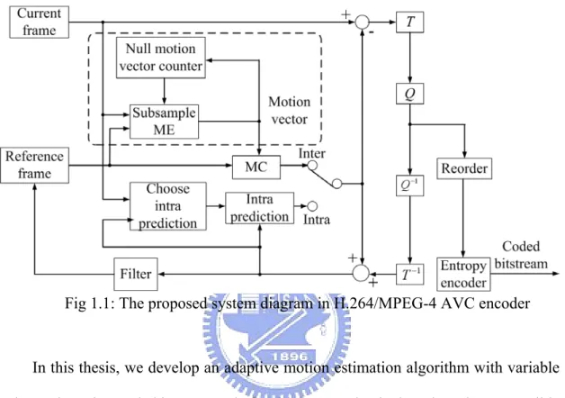
Fig 1.1: The proposed system diagram in H.264/MPEG-4 AVC encoder ....3 Fig 2.1: Rate-distortion curve comparison of H.264/MPEG-4 AVC with

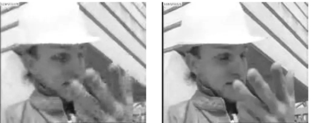
previous standards. (Excerpted from [22]) ...7 Fig 2.2: Subjective view comparison of MPEG-4 ASP (left) and

H.264/MPEG-4 AVC baseline (right) at bit-rate 112Kbps. (Excerpted from [22])...8 Fig 2.3: Block diagram of H.264/MPEG-4 AVC encoder...8 Fig 2.4: Segmented macroblock: Base block is 4x4. (Excerpted from [21])

...10 Fig 2.5: Variable block sizes in H.264/MPEG-4 AVC [4] (a) Macroblock

mode. (b) 8×8 mode. (Excerpted from [21]) ...10 Fig 2.6: One-dimensional array VBSME architecture in the paper [21].

(Excerpted from [21]) ...11 Fig 2.7: Process element of the FS-VBSME architecture in [21] (Excerpted

from [21])...12 Fig 2.8: Pixel patterns for decimation. (a) Full pattern with N×N pixels

selected. (b) Quarter pattern uses 4:1 subsampling. (c) Four-queen pattern is tiled with four identical patterns. (d) Eight-queen pattern. (c) and (d) are derived from the N-queen approach with N = 4 and N = 8, respectively. (Excerpted from [14])...15 Fig 2.9: (a) Patterns of pixels used for computing the matching criterion with

a 4 to 1 subsample ratio. (b) Alternating schedule of the four pixel subsample patterns over the search area (Excerpted from [12])...16

...20 Fig 2.12: (a) 1-D Hilbert sequence converted from Fig 2.11. (b) Edge pixels detected from 1-D Hilbert sequence. (c) 1-D row sequence converted from Fig 2.11. (d) Edge pixels detected from 1-D row sequence

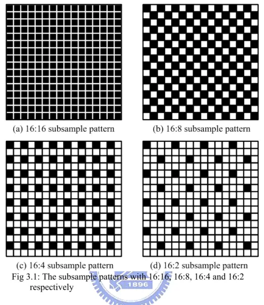
(Excerpted from [17]) ...22 Fig 3.1: The subsample patterns with 16:16, 16:8, 16:4 and 16:2 respectively

...25 Fig 3.2: The results ∆PSNRY of testing sequences “Dancer“, “Foreman“,

“Flower“, “Table“, “Mother Daughter“ and “Weather“...27 Fig 3.3: The results ∆PSNRY of testing sequences “Children“, “Paris“,

“News“, “Akiyo“, “Silent“ and “Container“ ...27 Fig 3.4: Frequency-domain illustration of down-sampling (Excerpted from

[18])...29 Fig 3.5: The diagram of ∆Q with 16:8, 16:4, 16:2 subsample ratios for table

sequence...32 Fig 3.6: The NMVC of the first P-frame in each GOP for table sequence..32 Fig 4.1: The flowchart of the proposed algorithm (Th16:2 is the threshold

between 16:2 subsample ratio and 16:4 subsample ratio, Th16:4 is the threshold between 16:4 subsample ratio and 16:8 subsample ratio and Th16:8 is the threshold between 16:8 subsample ratio and 16:16

Fig 4.2: The twelve testing video sequences ...41 Fig 4.3: The statistical distribution of ∆Q_GOP versus NMVC for twelve video

sequences ...41 Fig 4.4: Flow chart of the threshold decision algorithm...42 Fig 4.5: The distribution of threshold values ...43 Fig 5.1: Te average quality degradation of each GOP for the video sequence “table” ...47 Fig 5.2: The results ∆PSNRY of testing sequences “Dancer“, “Foreman“,

“Flower“, “Table“, “Mother Daughter“ and “Weather“ and the proposed algorithm results location...52 Fig 5.3: The results ∆PSNRY of testing sequences “Children“, “Paris“,

“News“, “Akiyo“, “Silent“ and “Container“ and “Weather“ and the proposed algorithm results location...52 Fig 5.4: The results ∆PSNRY of testing sequences “Dancer“, “Foreman“,

“Flower“, “Table“, “Mother Daughter“ and “Weather“ and the proposed algorithm results location in FME mode [38]...56 Fig 5.5: The results ∆PSNRY of testing sequences “Children“, “Paris“,

“News“, “Akiyo“, “Silent“ and “Container“ and “Weather“ and the proposed algorithm results location in FME mode [38] ...57

for horizontal, vertical and diagonal directions, there are eight, eight, and 15 possible edges, respectively, while for the diagonal directions, there are 15 possible edges. (Excerpted from [14]) ...18 Table 2 Threshold Setting of the adaptive subsample ratio threshold decision

...44 Table 3 Testing Video Sequences and Simulation Conditions...46 Table 4 Analysis of quality degradation using adaptive subsample ratio

decision ...49 Table 5 The simulation results of average subsample ratio and overall

average subsample ratio...49 Table 6 The PSNRY of the proposed algorithm and generic subsample ratio

algorithm...51 Table 7 The ∆PSNRY of the proposed algorithm and generic subsample ratio algorithm...51 Table 8 The result of the proposed algorithm in FME mode [38] ...55 Table 9 The PSNRY of the proposed algorithm and generic subsample ratio

algorithm in FME mode [38] ...55 Table 10 The ∆PSNRY of the proposed algorithm and generic subsample

Chapter 1 Introduction

In modern video standard, such as MPEG-1 [1], MPEG-2 [2], MPEG-4 [3] and H.264/MPEG-4 AVC [4], motion estimation requires the heaviest computational load and hence dominates main power requirement in video compression. Lots of published papers [4]-[17] and [39]-[47] have presented efficient algorithms for motion estimation. But they don’t consider the influence of the video content. In our observation, the video content effects on the performance of motion estimation. So we base on the video content to select the suitable motion estimation in order to achieve the best tradeoff between the power and quality. We think that we must use the different motion estimation in the different degree of the video content. Among these fast algorithms [4]-[17], the subsample algorithms [11]-[17] and [39]-[47] can not only easily combine with other approaches mentioned above but also reduce the number of matching points with flexibly changing subsample ratio.

The subsample algorithm, also called the pixel decimation algorithm, can be, in general, classified into two categories. One is fixed patterns [11]-[15], and the other is adaptive patterns [16] [17]. Bierling used an orthogonal sampling lattice with a 4:1 subsample [11]. Liu and Zaccarin implemented pixel decimation that is similar to Bierling’s approach with four alternating subsample patterns selected for each step so that all the pixels in the current block are visited [12]. T.Chiang et al presented an

N-queen decimation approach to address the spatial homogeneity and directional

coverage [14], [15]. The pixel decimation can be adapted based on the spatial luminance variation within a picture [16], [17]. The content-based subsample algorithm is proposed in [39]-[47]. Adaptive techniques can achieve better coding efficiency as compared to the uniform subsample schemes with an overhead in

subsample algorithms [16], [17] use the adaptive subsample patterns based on the spatial luminance variation within a picture, they all don’t mention the temporal variation. They result in serious aliasing problems in high frequency band to degrade the visual quality without considering the temporal variation. The temporal variation in the video means the degree of object-moving. The degree of object-moving is faster, and the temporal variation is stronger. Although the low subsample ratio cause aliasing in high frequency band, the degree of temporal variation will affect the degree of quality degradation. If the temporal variation is strong, aliasing problems will degrade the validity of motion vector (MV) and result in visual quality degradation to video sequences obviously. On the contrary, if the temporal variation is weak, aliasing problems will not degrade the validity of motion vector (MV) although the low subsample ratio still cause aliasing in high frequency band. That is because we do not need the high frequency band information to find the motion vector when the degree of object-moving is slow. Hence, using higher subsample ratio to reduce the prediction residual is necessary when temporal variation is stronger. In DSP theory [18] the subsample process will induce the aliasing in high frequency band. The aliasing problem affects the variance of the prediction residual under a fixed bit-rate constraint. The variance of the prediction residual affects the compression quality. The quality degradation of 0.5 dB is empirically reasonable for the perceptual tolerance of decompressed visual quality in video coding community. Therefore, in order to efficiently alleviate the aliasing problem to satisfy the visual quality under the quality

threshold of 0.5 dB for general video sequences, adaptively selecting the suitable subsample ratio according to the degree of temporal variation in the content is imperative.

Fig 1.1: The proposed system diagram in H.264/MPEG-4 AVC encoder

In this thesis, we develop an adaptive motion estimation algorithm with variable subsample ratios and this proposed algorithm can adaptively select the compatible subsample ratio for each current group of picture (GOP). The proposed algorithm is first to analyze the degree of the object-moving between the first P-frame and I-frame for the current GOP and then adaptively selects the suitable subsample ratio to the current GOP according to analysis result. The proposed algorithm also has been successfully implemented in the encoder model of H.264/MPEG-4 AVC [4] reference software JM9.2 [36] and the proposed system diagram is shown in Fig 1.1. The dash-lined region is the proposed motion estimation algorithm and the proposed algorithm offers four kinds of subsample ratios to adaptively switch. We use the statistics science to analyze every GOP degradation and null motion vector count (NMVC). And we get several different threshold values to experiment with video

in chapter 2. In chapter 3, we introduce the generic subsample algorithm in detail and describe the aliasing problem in the subsample algorithm. Chapter 4 describes the proposed algorithm. Chapter 5 shows the experimental performance of the proposed algorithm in H.264/MPEG-4 AVC [4] software model JM9.2 [36]. Finally, Chapter 6 concludes our contribution and merits of this work.

Chapter 2 Background

In this chapter, technical overview of H.264/MPEG-4 AVC [4] will be introduced [19] [20]. The feature of H.264/MPEG-4 AVC [4] unlike MPEG-4 [3] will be pointed out [19] [20]. The variable block size motion estimation is the main different place in H.264/MPEG-4 AVC [4]. The paper [21] proposed the new one-dimensional (1-D) very large-scale integration architecture for full-search VBSME (FSVBSME). About the full-search algorithm, it is particularly attractive to ones who require extremely high quality. However, it requires a huge number of arithmetic operations and results in highly computational load and power dissipation. In order to reduce the computational complexity of the FSBM, lots of published papers [4]-[17] and [39]-[47] have presented efficient algorithms for motion estimation. Among these fast algorithms [4]-[17] and [39]-[47], the subsample algorithms [11]-[17] and [39]-[47] can not only easily combine with other approaches mentioned above but also reduce the number of matching points with flexibly changing subsample ratio. In general, the subsample algorithm, also called the pixel decimation algorithm, can be classified into two categories. One is fixed patterns [11]-[15], and the other is adaptive patterns [16] [17] and [39]-[47]. Adaptive techniques can achieve better coding efficiency as compared to the uniform subsample schemes with an overhead in deciding which pattern is more representative. These presented subsample algorithms [11]-[17] and [39]-[47] can successfully reduce the computational complexity of motion estimation to save much power dissipation.

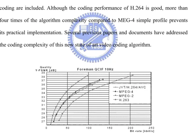
H.264/MPEG-4 AVC [4] with previous video coding standards. Under medium bit-rate, its PSNR quality outperforms MPEG-4 [3] simple profile by more than 3dB. Fig 2.2 shows H.264 baseline subjective view comparison with MPEG-4 advanced simple profile at the specification of QCIF and bit-rate 112Kbps.

H.264/MPEG-4 AVC [4] has such high performance because it adopts several novel coding tools in its algorithm design. For example, variable block size motion estimation, multiple reference frame motion estimation, and intra frame prediction are used in its prediction algorithm. In-loop deblocking filter offers good subjective view. The 6-tap filter is incorporated to do the quarter pixel interpolation. CAVLC (Context-Adaptive Variable Length Coding) and CABAC (Context-Adaptive Binary Arithmetic Coding) are adopted in its entropy coding design. H.264/MPEG-4 AVC [4] is the first video coding standard that adopts the arithmetic coding into its entropy design. The block diagram of H.264/MPEG-4 AVC encoder is shown in Fig 2.3. Video frames are captured into intra prediction and inter prediction parts. If the frame type is intra, the inter prediction part will be disabled. Multiple reference frames and variable block size motion estimation is used for inter prediction. The best mode among these prediction modes is chosen in the mode selection block. The input frame is then subtracted from the prediction and forms the residue block. The residue blocks are transformed by 4x4 integer DCT for luminance and 2x2 transform for chrominance DC coefficient. Scan and quantization procedures are then applied to the coefficients. The entropy coder receives these quantized coefficients and generates

codeword. The mode information is also transformed by the mode tables and fed into the entropy coder. The reconstruction loop includes the dequantization, inverse transform and deblocking filter. Finally, the reconstruct frame is written to the frame buffer for motion estimation.

There are three kinds of profile for H.264/MPEG-4 AVC standard [4]: baseline profile is for real-time communication, main profile is for digital storage application, and x-profile is for network streaming application. In the baseline profile, B-frame is not used and CAVLC is adopted in entropy coding. In the main profile, B-frame coding is used and CABAC is adopted for entropy coding. And X-profile has all the features of baseline profile while B-frame coding, SI-frame coding, and SP-frame [23] coding are included. Although the coding performance of H.264 is good, more than four times of the algorithm complexity compared to MEG-4 simple profile prevents its practical implementation. Several previous papers and documents have addressed the coding complexity of this new state of art video coding algorithm.

Fig 2.1: Rate-distortion curve comparison of H.264/MPEG-4 AVC with previous standards. (Excerpted from [22])

Fig 2.2: Subjective view comparison of MPEG-4 ASP (left) and

H.264/MPEG-4 AVC baseline (right) at bit-rate 112Kbps. (Excerpted from [22])

Fig 2.3: Block diagram of H.264/MPEG-4 AVC encoder.

Next section, we will discuss the architecture of motion estimation. And we will focus on the full-search variable block size motion estimation architecture.

2.2 Full-search Variable Block Size Motion estimation Architecture

(FS-VBSME)

The computational requirements for motion estimation are heavy and a real-time video application usually requires a direct mapped hardware architecture. Direct mapped architectures also have important advantages in terms of reduced power dissipation. Full-search algorithms, typically, can be implemented using regular 1-D

or 2-D systolic or systolic-like architectures as described by the paper [24]. 1-D systems offer a number of attractive features over their full 2-D counterparts, in particular much less complex data scheduling and simpler structures. These architectures are therefore attractive for portable devices because of their lower silicon area. The paper [25] has also demonstrated that flexible 1-D systems can be used to implement other fast matching algorithms, such as a three-step search (TSS) and pixel subsample.

To date, conventional VLSI architectures for computing variable block size motion estimation (VBSME) have been based on 2-D processor systems. For example, the architecture in the paper [26] uses a 2-D array with appropriate through masking of process elements (PEs). However, this results in low processor utilization. The architecture in the paper [27] uses a smaller 2-D array with partial-sum the sum of absolute difference (SAD) calculations performed sequentially using the smallest block size, 8×8. However, these architectures do not incorporate the capability to process all the variable block sizes (VBSs).

In H.264/MPEG-4 AVC [4], a macroblock is further segmented with the smallest block size being 4×4, as shown in Fig 2.4. This has two modes, the macroblock mode and the 8×8 mode. They are illustrated in Fig 2.5(a) and (b), respectively. VBSs must be accommodated, namely 4×4, 4×8, 8×4, 8×8, 16×8, 8×16, and 16×16. Referring to Fig 2.5(b), it will be noted that there are four quarter-blocks in a macroblock, each of which contains nine block patterns i.e., a total of 36 block patterns. However, observed in Fig 2.5(a), each macroblock contains another nine block patterns, with four of the 8×8 blocks common with the equivalent 8×8 blocks in Fig 2.5(b). Therefore, the total number of block patterns, to be processed is 36+9-4=41 i.e., a total of 41 motion vectors.

Fig 2.4: Segmented macroblock: Base block is 4x4. (Excerpted from [21])

Fig 2.5: Variable block sizes in H.264/MPEG-4 AVC [4] (a) Macroblock mode. (b) 8×8 mode. (Excerpted from [21])

The architecture presented in the paper [21] is based on 1-D array processor, in this case containing 16 PEs, in general, N for an N×N macroblock. This is summarized in Fig 2.6. A key aspect of the approach proposed is that it incorporates within the basic PE the means to accumulate the partial SAD values through shuffling. The scheduling of the current macroblock data (CMD) and search region data (SRD) is similar to a conventional 1-D architecture [28] with the CMD arranged in a raster scan sequence and the SRD arranged in a dual raster scan sequence. They apply this approach to the macroblock shown in Fig 2.4 and result in 16 SADs being computed, each with block size 4×4. The stored SADs are then re-used to compute SAD values for other block sizes. This is done by shuffling and combining the computed sub-block SAD values appropriately to derive SADs for each of the other larger

blocks sizes. For example, the results of two 4×4 sub-block computations can be combined to derive results for a 4×8 or 8×4 computation, and so on. This avoids the need to compute each of these from scratch and allows the overall computational requirements to be significantly reduced by avoiding the need to derive sub-block computation values that already have been established. As discussed below, this allows up to 41 VBS SAD values to be processed in a single processor.

Fig 2.6: One-dimensional array VBSME architecture in the paper [21]. (Excerpted from [21])

These computations of VBS’s SAD are performed using the internal PE circuitry. Details of which are shown in Fig 2.7. This uses a three stage process, provides 100% PE efficiency and allows SAD value computation to be choreographed directly with the data flow within the image. The first stage in the PE contains hardware to derive absolute difference values between the CMD and the SRD. These values are then latched to a second stage where they are multiplexed appropriately and stored in one of eight registers. The function of the registers and Mux C is to ensure that once computations have been performed these are stored and fed back in the correct order to compute the overall AD values for each of the sub-blocks 4×4. The function of the second stage of the array is twofold. The first is simply to pass, on successive cycles, the values 4×4 downwards through the PE cell. The second is to combine these values

values stored in the stage 2 registers via Mux D and Mux F. The net result is that by clock cycle 261 (256 cycles plus 5 cycles internal cell latency) all 41 candidate MVs are available from each PE.

Fig 2.7: Process element of the FS-VBSME architecture in [21] (Excerpted from [21])

Once all the values from an image block have been input then the data from a new block can immediately be input to each PE. This thus provides a continuous

streaming process that directly synchronizes with a constant flow of image data and means that each PE is 100% utilized. With 16 PEs working concurrently, the architecture described allows a total of 256 candidate MVs (16 16 search region) per sub-block to be processed in parallel with each PE producing all the information needed for a full search every 256 clock cycles— the same as existing architectures. However, in this case, this is done through the derivation of 41 MVs rather than one for each macroblock. Repeating this further 16 times means that up to 4096 clock cycles are required to complete a full search.

2.3 The Subsample Algorithm Using Fixed Pattern

The subsample algorithms [11]-[17] can not only easily combine with other approaches mentioned above but also reduce the number of matching points with flexibly changing subsample rate. For the fixed pattern, we can be sure that the power dissipation will be down by subample scale. But different patterns will case the different degreed of quality degradations.

Bierling used an orthogonal sampling lattice with a 4:1 subsample [11]. The pattern they used is the quarter pattern, shown in Fig 2.8 (b) [14]. The quarter pattern can save the power dissipation for 75%. And the paper [12] uses four different quarter pattern to the different search area. They are based on motion-field and pixel subsample. They first determine a subsample motion field by estimating the motion vectors for a fraction of the blocks. The motion vectors for these blocks are determined by using only a fraction of the pixels at any searched location and by alternating the pixel subsample patterns with the searched locations. They then interpolate the subsample motion field so that a motion vector is determined for each block of pixels. Fig 2.9 (a) shows a block of 8×8 pixels with each pixel labeled a, b, c,

computation, the use of this subsample pattern alone can seriously affect the accuracy of the motion vectors. To reduce this drawback, they proposes using all four quarter patterns, but only one at each location of the search area and in a specific alternating manner. Fig 2.9 (b) shows some pixels forming part of the search region in the previous frame. The pixels are labeled 1, 2, 3, and 4 in a regular pattern. The labeling of the pixels refers to which of the four quarter patterns of Fig 2.9 (a) is to be used for computing the matching at that location. That is, when computing the match at locations labeled 1 (i.e., when the upper-left pixel of the block to match falls on those locations), pattern A is used. Similarly, pattern B, C, or D is used when computing the match at locations labeled 2, 3, or 4.

Fig 2.8: Pixel patterns for decimation. (a) Full pattern with N×N pixels selected. (b) Quarter pattern uses 4:1 subsampling. (c) Four-queen pattern is tiled with four identical patterns. (d) Eight-queen pattern. (c) and (d) are derived from the N-queen approach with N = 4 and N = 8, respectively. (Excerpted from [14])

Fig 2.9: (a) Patterns of pixels used for computing the matching criterion with a 4 to 1 subsample ratio. (b) Alternating schedule of the four pixel subsample patterns over the search area (Excerpted from [12])

We can analyze the subsample pattern with the spatial homogeneity and directional coverage [14]. The spatial homogeneity is measured by the average and variance of spatial distances from each skipped pixel to its nearest selected pixel where N is the dimension of the block, and indicates the coordinates of the selected pixel nearest to the pixel at the position . K is the number of the selected pixels. Smaller ) , ( yx S ) , ( yx d

µ and indicate a more spatially homogeneous sampling lattice. An edge is defined as a line passing through the sampling grids in any of , , and directions in Fig 2.8 (d). The directional coverage is measured as the percentage of edges that at least one of the selected pixels exists on an edge. Table I shows that the quarter pattern has less spatial homogeneity and lacks half of the coverage in the specified directions. To address the issues of spatial homogeneity and directional coverage, the paper [14] construct a new N-queen sampling lattice Fig 2.8 (c) and (d). 2 d σ ° 0 45° 90° 135°

(

)

∑

∑

= = = = − − − = − − = N y x d d N y x d y x S y x K N y x S y x K N 1 , 1 2 2 2 1 , 1 2 ) , ( ) , ( ) ( 1 ) , ( ) , ( ) ( 1 µ σ µ (Excerpted from [14])

In the paper [14], to fully represent the spatial information of a N×N block, it is required that at least one pixel should be selected for each row, column, and diagonal. To satisfy such a constraint, the solution is identical to the problem of placing queens on a chessboard, which is referred to as -queen pattern. For a N×N block, as shown in Fig 2.8 (c) and (d), every pixel of the N-queen pattern occupies a dominant position, which is located at the center. All the other pixels located on the four lines in the vertical, horizontal and diagonal directions are removed from the list of the selected pixels. With such elimination process, there is exactly one pixel selected for each row, column, and (not necessarily main) diagonal of the block. Thus, the N-queen patterns present a subsample lattice that can provide N times of speedup improvement. Despite the randomized lattice, the paper [15] designed compact data storage architecture for efficient memory access and simple hardware implementation for the N-queen patterns.

d d µ Full 0 0 8/8 8/8 15/15 15/15 Quarter [11] 1.14 0.04 17.16% 4/8 4/8 7/15 7/15 Hexagonal [13] 1.03 0.11 11.07% 4/8 8/8 12/15 12/15 4-Queen [14] 1 0 8/8 8/8 10/15 10/15 8-Queen [14] 1.32 0.14 28.77% 8/8 8/8 8/15 8/15

2.4 The Subsample Algorithm using adaptive Pattern

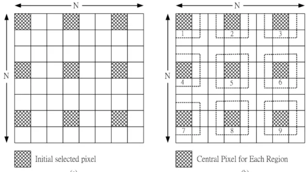
The approach using the fixed patterns could possibly be able to obtain a good estimation of motion when the intensity of the block is nearly uniform. However, in the case of high activity blocks, some details may be neglected. Thus, it probably would introduce excessive prediction error. The paper [16] is based on the fact that high activity in spatial domain such as edges and texture mainly contributes to the MAD criterion. We can vary the number of selected pixels based on the image details. In other words, we can use fewer pixels when the block has uniform intensity. But in the high activity block, more pixels can be employed for the MAD matching criterion. This adaptive approach [16] can reduce the prediction error compared with standard pixel decimation [11]-[15]. In the algorithm [16], they used the relationship between a pixel and its neighbors to select the most representative pixels. For example in 8×8 block size, initially, nine pixels are selected as shown in Fig 2.10 (a). The 8 x 8 pixel

block is divided into nine regions, depicted in Fig 2.10(b), and each region has its corresponding central pixel. In each region, the difference is defined the difference between central pixel and one of its neighbor pixels. If the difference is greater than threshold, this pixel is selected. We have used block size of 8 x 8 as an example for the description of the proposed algorithm in the paper [16], however, the extension of the proposed scheme to a large block size, say 16 x 16, is straightforward.

k D k D K k k h k I h k I

D ( , )= ( , )− , where (h, k) is the location of the neighbor pixel in

region K, with (h, k) as the displacements from the central pixel . I_k

Fig 2.10: Adaptive pixel selection (a) nine selected pixels. (b) The selected pixels in (a) are considered as the central pixel for each region, the dotted lines indicate the neighbor pixels of respective central pixels in each region. (Excerpted from [16])

Fig 2.11: An edge in a 16×6 block for testing the subsample algorithm [17]

About the paper [16], their scheme still requires an initial uniform division of a block, and therefore the pattern is locally adaptive. The pixel-decimation algorithm proposed in the paper [17] also utilizes edge information. Compared to Chan’s method [16], it extends the adaptivity from local to global. To realize global adaptivity, the algorithm [17] looks directly for edge pixels instead of requiring an initial uniform division of a block. This task [17] is made easier in a 1-D space with the help of Hilbert scan [29]. The Hilbert scan was named after the great German mathematician Hilbert, who found the simplest family of curves (Hilbert curves) that pass through all the grid points only once in a 2-D space [29]. The Hilbert scan, defined as a scan of a 2-D image through one of its Hilbert curves, is equivalent to a depth-first scanning of a quad-tree representation of the 2-D image. Some interesting features of this scan method used in previous applications include: 1) it is easier to extract clusters in an image with a Hilbert scan than other scan methods, e.g., row scan, row-prime scan, Morton scan, etc., and 2) it preserves 2-D coherence [30]–[35]. In addition, Kamata has shown that edge information in a 2-D image is preserved in its 1-D Hilbert-scan sequence, and has demonstrated an effective compression of 2-D images by compressing their 1-D sequences using the edge information [34]. The compressed images have a similar visual quality to that of the JPEG images at a high

compression rate.

To illustrate how edges are detected in a 1-D Hilbert sequence, Fig 2.11 shows a 2-D block with a closed circular edge, and Fig 2.12 (a) is the 1-D Hilbert sequence converted from the block in Fig 2.11. If edge pixels are defined at where pixel intensity changes the most, 22 edge pixels can be located in Fig 2.12 (a). All of the 22 pixels, when mapped back to 2-D, appear evenly distributed on the circular edge as shown in Fig 2.12 (b). For comparison, Fig 2.12 (c) is the 1-D row sequence converted from the same block in Fig 2.11. Although the row sequence contains 20 edge pixels, they all appear at the left and right vertical portion of the circular edge, and none appear on the upper and lower horizontal edges, as shown in Fig 2.12 (d). In general, the Hilbert scan not only provides edge information with little directional preference, but also preserves pixel coherence more effectively than other scan methods. In contrast, row scan, typical of many other scan methods, may miss edges due to its scan direction. Based on edge information in 1-D Hilbert sequences [29], the algorithm [16] selects pixels at which the matching criterion is evaluated.

Fig 2.12: (a) 1-D Hilbert sequence converted from Fig 2.11. (b) Edge pixels detected from 1-D Hilbert sequence. (c) 1-D row sequence converted from Fig 2.11. (d) Edge pixels detected from 1-D row sequence (Excerpted from [17])

The paper [39]-[47] proposed that the general subsample algorithm has aliasing problem when it is in high subsample rate. The aliasing problem leads to considerable quality degradation because the high frequency band is messed up. To alleviate the problem, he uses edge extraction techniques to separate the edge pixels from a macro-block and then perform subsampling to the remaining pixels.

Although the subsample algorithms [11]-[17] and [39]-[47] reduce the number of matching points with flexibly changing subsample rate to save the power dissipation, they will cause the aliasing problem in high frequency band. Next, we will explain aliasing problems in subsample algorithms.

Chapter 3 Aliasing Problems in Subsample

Algorithm

In this chapter, we present a generic subsample algorithm in which the subsample ratio ranges from 16-to-2 to 1-to-1. We use the fixed subsample ratio to test the video sequences and observe that the quality degradation is dependent on the video content. That is because the subsample process will induce the aliasing in high frequency band [18]. The video with high motion have the high quality degradation. On the contrary, the video with low motion have the low quality degradation. We discuss aliasing problems in subsample algorithms in this chapter. From DSP theory [18], we will kwon the reason why aliasing problems happen. We also can find this situation in every GOP of the video sequence. We assume that the frames in the GOP are very correlative. So we can see the GOP as a control unit to adaptively select the best subsample ratio. Aliasing problems can be solved more accurate. And the video sequence “Table” is the example to explain the relationship between the quality degradation and the video content in aliasing problems in high frequency band.

3.1 Generic Subsample Algorithm

Here, we present a generic subsample algorithm in which the subsample ratio ranges from 16-to-2 to 1-to-1. The basic operation of the generic subsample algorithm is to find the best motion estimation with less SAD computation. The generic subsample algorithm uses Eq.1 as a matching criterion, called as subsample sum of absolute difference (SSAD), where the macro-block size is N-by-N, is the

luminance value at of the current macro-block (CMB). The is

) , ( ji R ) , ( ji S(i+u, j+v)

The other subsample patterns are omitted because they also can be generated from the generic subsample algorithm and the subsample patterns of 16:16, 16:8, 16:4 and 16:2 shown in Fig 3.1 are symmetry and their scale is power of two.

( )

[

]

) 2 ( 8 , 7 , 6 , 5 , 4 , 3 , 2 , 1 ), 4 mod , 4 mod ( ) , ( ) 1 ( 1 , , ) , ( ) , ( ) , ( , 2 : 16 2 : 16 1 0 1 0 2 : 16 2 : 16 = = − ≤ ≤ − − + + ⋅ =

∑∑

− = − = m j i BM j i SM p v u p for j i R v j u i S j i SM v u SSAD n m N i N i m SM m

( )

⎩ ⎨ ⎧ < ≥ = ⎥ ⎥ ⎥ ⎥ ⎦ ⎤ ⎢ ⎢ ⎢ ⎢ ⎣ ⎡ − − − − − − − − − − − − − − − − = 0 , 0 0 , 1 ) ( , : ) 3 ( ) 4 ( ) 8 ( ) 3 ( ) 7 ( ) 6 ( ) 1 ( ) 5 ( ) 2 ( ) 4 ( ) 8 ( ) 3 ( ) 7 ( ) 6 ( ) 2 ( ) 5 ( ) 1 ( 2 : 16 n for n for n u is that function step a is n u when m u m u m u m u m u m u m u m u m u m u m u m u m u m u m u m u BM _m

Fig 3.1: The subsample patterns with 16:16, 16:8, 16:4 and 16:2 respectively

Given a subsample mask generated from Eq.3, the computational cost of SSAD can be lower than that of SAD. Hence, the generic subsample algorithm can achieve the target of power-saving with flexibly changing subsample ratio. However, the generic subsample algorithm suffers form aliasing problems in high frequency band. Aliasing problems will degrade the validity of motion vector (MV) and result in visual quality degradation to video sequences obviously.

We use the fixed subsample ratio from 16:2 to 1:1 to experiment the twelve video sequences [37] in H.264/MPEG-4 AVC [4] coder with JM9.2 [36]. Here, we define one group of picture (GOP) is fifteen frames, frame rate is 30 frames/s, the bit rate is 450k bits/s and initial Qp is 34. We can observe the quality degradation of the video sequence in the Fig 3.2 and Fig 3.3. In Fig 3.2, the video sequence “dancer” has

degradation acceptable. The quality degradation of 0.5 dB is empirically reasonable for the perceptual tolerance of decompressed visual quality in video coding community. Therefore, we can conclude that we must use the difference subsample ratio to keep the quality degradation acceptable. It is not enough to only use the fixed subsample pattern for all video sequences. From Fig 3.3, the most quality degradation is not over the 0.35 dB. We call those video sequences as low motion video sequences. They have the low degree of temporal variation. The temporal variation in the video means the degree of object-moving. The degree of object-moving is faster, and the temporal variation is stronger. Although the low subsample ratio cause aliasing in high frequency band, the degree of temporal variation will affect the degree of quality degradation. If the temporal variation is strong, aliasing problems will degrade the validity of motion vector (MV) and result in visual quality degradation to video sequences obviously. On the contrary, if the temporal variation is weak, aliasing problems will not degrade the validity of motion vector (MV) although the low subsample ratio still cause aliasing in high frequency band. That is because we do not need the high frequency band information to find the motion vector when the degree of object-moving is slow. Hence, using higher subsample ratio to reduce the prediction residual is necessary when temporal variation is stronger. For those video sequences, unlike the video sequences in the Fig 3.2, we can use the lowest the subsample ratio to save the largest power dissipation. That is because the quality degradation is acceptable.

Fig 3.2: The results ∆PSNRY of testing sequences “Dancer“, “Foreman“, “Flower“, “Table“, “Mother Daughter“ and “Weather“

Fig 3.3: The results ∆PSNRY of testing sequences “Children“, “Paris“, “News“, “Akiyo“, “Silent“ and “Container“

3.2 Aliasing Problems in High Frequency Band

As mentioned above, the generic subsample algorithm has aliasing problems for low subsample ratio and leads to considerable quality degradation because the high frequency band is messed up.

The subsample process is like the down-sampling process in DSP theory [18]. In general, the operation of reducing the sampling ratio will be called down-sampling. Down-sampling is illustrated in Fig 3.4. We assume that the Fig 3.4 (a) is the conceptual spectrum of a macroblock in a frame of a video sequence. If this macroblock is down-sampling by 2, then his new conceptual spectrum will be Fig 3.4 (b). Because the original conceptual spectrum is low bandwidth and the down-sampling ratio is high, the aliasing don’t happen in this case. If the down-sampling ratio becomes 3, the aliasing will happen shown in Fig 3.4 (c). The aliasing in the high frequency band will case the motion estimation is no accurate. Aliasing problems affect the variance of the prediction residual under a fixed bit-rate constraint. The variance of the prediction residual affects the compression quality. Therefore, in order to efficiently alleviate aliasing problems to satisfy the visual quality under the quality threshold of 0.5 dB for general video sequences, adaptively selecting the suitable subsample ratio according to the degree of temporal variation in the content is imperative.

(a) The original conceptual spectrum

(b) Down-sampling by 2

(c) Down-sampling by 3 (with aliasing problem)

Fig 3.4: Frequency-domain illustration of down-sampling (Excerpted from [18])

In all the twelve video sequences, the video sequences with low motion have no aliasing problems, like “Children“, “Paris“, “News“, “Akiyo“, “Silent“ and “Container“. About these video sequences, we can use the low subsample ratio in order to save the large power dissipation without the high quality degradation. That is because these video sequences have low frequency distribution and weak temporal variation. Although we down-sample the video sequences by large number, the high frequency don’t be messed up. On the other hand, the video sequences with high and normal motion have aliasing problems. If we down-sample those video sequences by large number, the quality degradation will be large. For example, the video sequence “Dancer” will case 0.93 dB quality degradation using the 16:2 subsample ratio. That quality degradation is very serious and can’t be acceptable.

subsample ratio results in more noticeable aliasing because of increasing the inaccurate moving motion vector count (MMVC) and furthermore increases prediction residual to degrade the visual quality in a bit rate control. Therefore, the high subsample ratio is necessary for a fast motion video. And the low subsample ratio is also suitable for a normal or slow motion video.

We define the null motion vector count to reflect the spectrum in frequency deomain. We use the lower of subsample ratio for the larger of NMVC. On the other hand, we use the higher of subsample ratio for the smaller of NMVC. The overhand of the point for the spectum is only an extra counter for implementation. But in the encode system, we get the NMVC value after encoding. But we have to decide the subsample ratio before encoding. In order to solve this problem, we use the GOP as a processing unit. For any video sequence, the degree of temporal variation in this video sequence is not the same. We also can find this situation in every GOP in the video sequence. The GOP is like the small size of video sequence, about 0.5 second. Because the number of frames in the GOP is smaller than that in the video sequence, we assume that the frames in the GOP are very correlative. So we can see the GOP as a control unit to adaptively select the best subsample ratio. If we do that, we can get the degree of temporal variation more accurate. Aliasing problems can be solved more accurate. So We get the NMVC of the first P-frame in the GOP as the point to select the suitable subsample ratio for this GOP. The more detail will be discuss in next

chapter.

We take the video sequence “Table” for example. To particularly analyze the results of visual quality degradation with different subsample ratios for a video, the normal motion video sequence “table” is simulated in H.264/MPEG-4 AVC [4] coder with JM9.2 [36]. Here, we define one group of picture (GOP) is fifteen frames, frame rate is 30 frames/s, the bit rate is 450k bits/s and initial Qp is 34. Subsample ratios are 16:8, 16:4 and 16:2 respectively and can be generated from Eq.3. Fig 3.5 shows quality degradation results versus these subsample ratios. Fig 3.6 shows the NMVC value of the first P-frame in each GOP. The average quality degradation of ith GOP ( ) is defined as shown in Eq.4, where is the average PSNRY of ith GOP using the full-search block-matching (FSBM). is the average PSNRY of ith GOP with specific subsample ratio (SSR). From Fig 3.5, there exists the stronger temporal variation between third GOP and seventh GOP, hence, the lower subsample ratio leads to more obviously aliasing problems and results in higher quality degradation. We can see the NMVC values of these GOPs are larger in Fig 3.6. This can reflect the the aliasing problem. Furthermore, the tenth GOP has maximum quality degradation because of scene change. Although lower subsample ratio leads to more obviously aliasing problems in high frequency band, Fig 3.5 also shows that quality degradation is unobvious between eleventh GOP and twenty GOP because of the weaker temporal variation. In Fig 3.6, the NMVC values of these GOPs are small. So we can use the NMVC to select the suitable subsample ratio for the GOP.

GOP ith Q ∆ PSNRY_{i FSME} SSR i PSNRY

(

_{i FSME i SSR}

)

(4) GOP

ith PSNRY PSNRY

Q = −

Fig 3.5: The diagram of ∆Q with 16:8, 16:4, 16:2 subsample ratios for table sequence.

From Fig 3.5 and Fig 3.6, the various degrees of temporal variation are distributed over GOPs even though the “table” video sequence is regarded as a normal motion video. Therefore, in order to efficiently alleviate the aliasing problems, we need develop an adaptive motion estimation scheme and this scheme can adaptively supply the suitable sample ratio to each GOP according to the degree of NMVC in order to maintain the better visual quality in a bit rate control.

process unit. We get the null motion vector count (NMVC) from the first P-frame in the current GOP. In order to make sure the correct of NMVC, we set the first P-frame in the GOP to use the full search motion estimation. That is 16:16 subsample ratio. According the value of NMVC, we select the suitable subsample ratio for the next 13 P-frames in the current GOP. Then the flowchart of the proposed algorithm is developed. Next, we provide four subsample ratios of 16:16, 16:8, 16:4 and 16:2 in order to let the proposed algorithm having better adaptive ability. The reason why to choose those subsample ratios is because they are symmetry and their scale is power of two. Final, we propose an adaptive subsample ratio threshold decision to set the compatible threshold values and get the optimal result. The static science is adopted in the adaptive subsample ratio threshold decision. We test the percentage of 90%-65% in the static data of the quality degradation versus NMVC to get the different threshold value. From the result of twelve testing video sequence, we take the 70% result as the optimal threshold value.

4.1 Proposed Algorithm Development

To efficiently alleviate the aliasing problems in subsample algorithm to maintain the visual quality under the threshold of 0.3 dB for general video sequences, we propose an adaptive motion estimation algorithm using variable subsample ratios and the proposed algorithm is based on the observation in Fig 3.4. From Fig 3.4, the

temporal variation in a frame is in proportion to moving motion vector count (MMVC), meaning that it is in inverse proportion to null motion vector count (NMVC). Therefore, we use one GOP as a processing unit and calculate the NMVC of the first P-frame in a processing unit. Next, we compare NMVC with threshold values to determine the suitable subsample ratio for the current GOP. We recursively execute these steps above, and we can adaptively supply the suitable subsample ratio to each GOP in one video sequence and also achieve the target of power saving.

A flowchart of the proposed algorithm is shown Fig 4.1 and the realization procedure of the adaptive motion estimation algorithm using variable subsample ratios is as follows.

Step 1: Setting initial value

Set i=1.

We set the initial value in this proposed algorithm. And the proposed algorithm is ready to start

Step 2: Starting

When starting the proposed algorithm, the ith GOP of current video sequence is picked out and the first frame of the ith GOP goes to Step 3.

In this step, we check the number of the frames in the GOP. We have to realize which frame is the first frame in the GOP and start our proposed algorithm from beginning. For the arrangement of a GOP, the first frame is coded using intra-prediction and the others are coded using inter-prediction. So, every GOP can be seen as a small size video sequence, about 0.5 second. But the advantage of this GOP is the high correlation between the frames in the GOP. That is why we choose the GOP as the process unit to adaptively select the suitable subsample ratio.

Step 3: Determining the current frame whether an I-frame or not

Step 4: Determining the current frame whether a first P-frame or not

If the current frame is a first P-frame, the proposed algorithm executes inter-frame coding for the current P-frame using 16:16 subsample ratio and then calculates the null motion estimation count (NMVC) of the current frame; otherwise, the current P-frame goes to Step 5.

The reason why the first P-frame in the GOP use the 16:16 subsample ratio is that we want the accurate NMVC. If the NMVC is not correct, the subsample ratio for the rest 13 P-frames will not be suitable for this GOP. It will cause the large quality degradation or waste the power dissipation for low motion GOP. Therefore, in order to get the correct NMVC, we consume the power to using the 16:16 subsample ratio.

Step 5: Adaptively selecting the suitable subsample ratio to the current P-frame

The proposed algorithm compares NMVC of the first P-frame with optimal threshold values to adaptively select a suitable subsample ratio and then uses this selected subsample ratio to execute inter-frame coding for the current P-frame and then the current P-frame goes to Step 6.

In this step, we process the rest 13 P-frames in the GOP. These frames will be code using the selected subsample ratio. The selected subsample ratio is according to the NMVC of the first P-frame in the GOP. We assume that the frames in the current GOP have the high correlation between each other. According to the NMVC of the first P-frame, we recognize the current GOP as high, normal or low motion GOP. And we compare this NMVC with the threshold value to decide the suitable subsample

ratio for the current GOP. The inter-prediction of the rest 13 P-frames uses this suitable subsample ratio.

Step 6: Determining the current P-frame whether a last P-frame or not

If the current P-frame is a last frame, the procedure goes to Step 7; otherwise, the next frame goes to Step 3.

When the current GOP is end, we have to start the proposed algorithm again and to control the next GOP. Otherwise, the frame in the current GOP will be coded according to the situation in the current GOP.

Step 7: Ending

If all GOPs in the current video sequence are encoded, the proposed algorithm finishes; otherwise, the procedure sets i=i+1 and goes to step 2;

This video is end and all frames in the video sequence have been coded using the proposed algorithm in the H.264/MPEG-4 AVC [4].

Fig 4.1: The flowchart of the proposed algorithm (Th16:2 is the threshold between 16:2 subsample ratio and 16:4 subsample ratio, Th16:4 is the threshold between 16:4 subsample ratio and 16:8 subsample ratio and Th16:8 is the threshold between 16:8 subsample ratio and 16:16 subsample ratio).

4.2 Subsample Patterns of the Proposed Algorithm

To demonstrate that the proposed algorithm has better adaptive ability, the proposed algorithm provides four subsample ratios and adaptively selects the suitable subsample ratio from these subsample patterns to the current GOP. These subsample ratios are fixed at powers of two in spatial distribution and are 16:16, 16:8, 16:4 and 16:2 respectively. These subsample masks can be generated in a 16-by-16 macro-block using Eq.3 and are shown in Fig 3.1. The reason why to choose those subsample ratios is because they are symmetry and their scale is power of two. We select four subsample ratios in our proposed algorithm. There are four levels of 16:16, 16:8, 16:4 and 16:2. All P-frames expect the first P-frame in the GOP will be classified into four levels according to the NMVC of the first P-frame in the GOP. Every GOP have only one subsample ratio. According to these subsample ratios, the proposed algorithm can adaptively select the suitable subsample ratio to the current GOP. For example, the proposed algorithm can provide the 16:16 subsample ratio for the current GOP which has the stronger degree of temporal variation or provide the 16:2 subsample ratio for the current GOP which has the weaker degree of temporal variation. The temporal variation in the video means the degree of object-moving. The degree of object-moving is faster, and the temporal variation is stronger. Although the low subsample ratio cause aliasing in high frequency band, the degree of temporal variation will affect the degree of quality degradation. If the temporal variation is strong, aliasing problems will degrade the validity of motion vector (MV) and result in visual quality degradation to video sequences obviously. On the contrary, if the temporal variation is weak, aliasing problems will not degrade the validity of motion vector (MV) although the low subsample ratio still cause aliasing in high frequency band. That is because we do not need the high frequency band information to find the

inter-prediction of the rest 13 P-frames uses this suitable subsample ratio. Therefore, a threshold decision for variable subsample ratios is necessary to set the compatible threshold values in order to adaptively choosing the suitable subsample ratio to the current GOP. Next, a threshold decision for variable subsample ratios will be presented in chapter 4.3.

4.3 Threshold Decision for Variable Subsample Ratios

To support a suitable subsample ratio to other P-frames of current GOP, except the first P-frame of the current GOP, an adaptive subsample ratio threshold decision is necessary. Therefore, we use 16:2, 16:4, 16:8 and 16:16 subsample ratios respectively to calculate the statistical distribution of ∆QGOP versus NMVC for twelve video

sequences (Fig 4.2) [37].

The statistical results are shown as in Fig 4.3 and each coordinate means

versus NMVC using a specific subsample ratio. From Fig 4.3, we can observe that the statistical distribution of versus NMVC focus on the right side. This situation means the most video sequence must have a part of background region. The background region means the MV is null. There is not video sequence without the background region except for scene change. For scene change case, there is no algorithm can be solved success.

GOP Q ∆ GOP Q ∆

“Dancer“ “Foreman“ ”Flower“ “Table“

“Mother Daughter“ “Weather“ “Children“ “Paris“

“News“ “Akiyo“ “Silent“ “Container“

Fig 4.2: The twelve testing video sequences

Fig 4.3: The statistical distribution of ∆Q_GOP versus NMVC for twelve

percentage of total using a selected subsample ratio and this method is proposed as Fig 4.4.

We first set the quality degradation threshold is 0.3 dB. We define the first region is the selected 16:2 subsample ratio. The second region is the selected 16:4 subsample ratio. The selected 16:8 subsample ratio is the third region. The last region, fourth region, is the selected 16:16 subsample ratio. In the first region, we calculate the percentage of the number of point with the quality degradation under 0.3dB using the 16:2 subsample ratio in this region. For the second region, the percentage of the number of point with the quality degradation under 0.3dB using the 16:2 subsample ratio change to 16:4 subsample ratio. And third region is for 16:8 subsample ratio. So we set the percentage threshold from 90% to 60%, every decreasing for 5%. We will get the seven forms of the adaptive subsample ratio threshold value.

To get the threshold values between these subsample ratios, we use the threshold decisions mentioned above to calculate the threshold values and the distribution of threshold values is shown as Fig 4.5. We can observe the size of every region directly in Fig 4.5.

Threshold of 16:8 (TH_16:8) 265 242 227 207 179 49 X

Table 2 shows the summary of threshold values using different adaptive subsample ratio decision. From the Table 2, we observe the adaptive subsample ratio threshold value of 60% is not complete. There is not the value. That is because the second region is too big and the rest region can make the percentage down to 60%. About the 65%, the value is too small so that the 16:16 subsample ratio is hardly selected. For the 90%, 85%, 80%, 75% and 70%, the first region increases. That means we can tolerate more change of the quality degradation over 0.3 dB. The same situation is happened in the second and third regions.

8 : 16 TH 8 : 16 TH

Chapter 5 Experimental Result

In our simulation, the proposed algorithm is simulated in H.264/MPEG-4 AVC [4] with software model JM9.2 [36] using AMD 2.0G Hz and the distortion measure is sum of absolute difference (SAD) which is computed for a 16-by-16 macro-block. We use twelve famous video sequences [37] to be tested and the simulation environment in JM9.2 is shown as in Table 3. From Table 3, the file format of these video sequences is CIF (352 × 288 pixels) and the search range is ±16 in both horizontal and vertical directions for a 16-16 macro-block. The bit-rate control is turned on to maintain a fixed bit rate of 450k bits/s under displaying 30 frames / s. In Chapter 4, we proposed an adaptive subsample ratio decision to pick the suitable subsample ratio and the adaptive subsample ratio threshold decision support six different threshold values between 16:16, 16:8, 16:4 and 16:2, which are shown as in Table 2. To choose the optimal threshold values from Table 2, we simulate these tested video sequences using these subsample ratio decisions respectively in the same simulation condition and then analysis to decide the optimal threshold values from these decisions based on two factors: average quality degradation (∆PSNRY) and average subsample ratio. The PSNRY is defined as Eq.5 where the frame size is N × M, and denote the Y components of original frame and reconstructed frame at (x; y). The ∆PSNRY is defined as Eq.6 and it means the difference of PSNRY which is calculated by a chosen algorithm and PSNRY which is calculated by using full-search block-matching algorithm (FSBM).

(

x y I_Y ,

)

Iˆ_Y

(

x,y

)

(

)

(

( )

( )

)

) 6 ( ) 5 ( , ˆ , 1 255 log 10 lg 2 2 10 FSME orithm a Chosen Y Y PSNRY PSNRY PSNRY y x I y x I M N PSNRY − = ∆ − ⎟ ⎠ ⎞ ⎜ ⎝ ⎛ × × =

∑∑

(

)

(

)

(

(

)

)

(

#

)

(7) ] 2 # 4 # 8 # 16 # [ : 16 2 : 16 4 : 16 8 : 16 16 : 16 frames P of Total frames P of frames P of frames P of frames P of − × − + × − + × − + × − = Table 3

Testing Video Sequences and Simulation Conditions Video Sequence Number of Frames Format Frame Rate (frames/s) Bit Rate (bits/s) Initail Qp Search Range GOP Unit Video Type Dancer 250 Foreman 300 Fast Motion Flower 250 Table 300 Mother Daughter 300 Weather 300 Children 300 Normal Motion Paris 300 News 300 Akiyo 300 Silent 300 Slow Motion Container 300 CIF (352 × 288) 30 450k 34 ±16 15 frames IPPP… IPPP…

To demonstrate that the proposed algorithm can adaptively select the suitable subsample ratio to each GOP for a tested video sequence, we analysis the average quality degradation of each GOP using Eq.4 for the video sequence “table” and the results is shown as in Fig 5.1. This case is the same with the Fig 3.4 in chapter 3. But the Fig 5.1 adds the distribution of the proposed algorithm to demonstrate the performance of the proposed algorithm. From Fig 5.1, there exists the stronger

temporal variation between third GOP and seventh GOP, the proposed algorithm can adaptively support higher subsample ratio to efficiently reduce the ∆GOP. Besides, the proposed algorithm can adaptively support lower subsample ratio to save power dissipation without affecting the ∆GOP between eleventh GOP and twenty GOP because of the weaker temporal variation.

Fig 5.1: Te average quality degradation of each GOP for the video sequence “table”

Table 4 shows the simulation results of PSNRY and ∆PSNRY for these tested video sequences using this threshold decision method. Table 5 shows the simulation results of average subsample ratio and overall average subsample ratio for these tested video sequences using this threshold decision method. Because threshold values of Table 2 can be calculated according to the target of average quality degradation of 0.3 dB, the average quality degradation of 0.3 dB is an important index for all tested video sequences. From Table 4 and Table 5, 90%, 85% and 80% statistics of threshold decision method can satisfy all tested video sequences under the average quality

dB. For the video sequences “Dancer” and “Mother Daughter”, their quality degradations in this 70% method are the same and are equal to 0.36 dB. And the quality degradation in this 70% method of video sequence “Foreman” is equal to 0.33 dB. For “Paris”, it is 0.35 dB. And 0.33 dB is for “Weather”. Although the overall average subsample ratio of 65% statistics of threshold decision method is the lowest, the average quality degradation of it exceeds 0.3 dB too much. For example, the average quality degradations of the sequences “Dancer” and “Foreman” are 0.77dB and 0.59 dB. These quality degradations are not acceptable. For the 70% statistics, we can observe the video sequences of fast motion have the maximum acceptable quality degradation for near 0.3 dB. In this quality degradation, the power consumption is the maximum. We can save the power efficiently. For the other threshold values, they can also keep the quality degradation acceptable. But they waste the power to gain the better quality degradation under 0.3 dB. For the low motion video sequences, the algorithm using the threshold value of 70% statistics can select adaptively the minimum power consumption to save power efficiently. The minimum power consumption is the average subsample ratio 16:3. That contains the number of the first P-frame in the GOP using 16:16 subsample ratio and all the rest P-frame using 16:2 subsample ratio. Therefore, in order to minimize the power consumption of motion estimation and maintain the average visual quality about 0.3dB, threshold values of 70% statistics is the optimal choice for adaptively selecting the suitable subsample ratio.And we save 69.6% power consumption and keep quality degradation under 0.36

dB.

Table 4

Analysis of quality degradation using adaptive subsample ratio decision The adaptive subsample ratio threshold decision

90% 85% 80% 75% 70% 65% Video Sequence Full Search PSNRY PSNRY Δ PSNRY PSNRY Δ PSNRY PSNRY Δ PSNRY PSNRY Δ PSNRY PSNRY Δ PSNRY PSNRY Δ PSNRY Dancer 33.42 33.4 -0.02 33.4 -0.02 33.4 -0.02 33.33 -0.09 33.06 -0.36 32.65 -0.77 Foreman 29.51 29.42 -0.09 29.36 -0.15 29.35 -0.16 29.2 -0.31 29.18 -0.33 28.92 -0.59 Fast Motion Flower 19.58 19.58 0 19.54 -0.04 19.54 -0.04 19.43 -0.15 19.31 -0.27 19.14 -0.44 Table 31.04 30.99 -0.05 30.98 -0.06 30.93 -0.11 30.85 -0.19 30.78 -0.26 30.7 -0.34 Mother Daughter 39.34 39.14 -0.2 39.12 -0.22 39.11 -0.23 39.01 -0.33 38.98 -0.36 38.89 -0.45 Weather 32.26 32.06 -0.2 32.04 -0.22 32.01 -0.25 31.97 -0.29 31.93 -0.33 31.93 -0.33 Children 29 28.87 -0.13 28.84 -0.16 28.81 -0.19 28.72 -0.28 28.71 -0.29 28.71 -0.29 Normal Motion Paris 30.67 30.5 -0.17 30.45 -0.22 30.46 -0.21 30.36 -0.31 30.32 -0.35 30.32 -0.35 News 37.27 37.19 -0.08 37.17 -0.1 37.15 -0.12 37.12 -0.15 37.07 -0.2 37.07 -0.2 Akiyo 42.36 42.27 -0.09 42.24 -0.12 42.24 -0.12 42.21 -0.15 42.21 -0.15 42.21 -0.15 Silent 34.62 34.56 -0.06 34.57 -0.05 34.58 -0.04 34.56 -0.06 34.53 -0.09 34.53 -0.09 Slow Motion Container 35.47 35.45 -0.02 35.45 -0.02 35.45 -0.02 35.45 -0.02 35.45 -0.02 35.45 -0.02 Table 5

The simulation results of average subsample ratio and overall average subsample ratio

Threshold Decision 90% 85% 80% 75% 70% 65% Video Sequence Average Subsample ratio Average Subsample ratio Average Subsample ratio Average Subsample ratio Average Subsample ratio Average Subsample ratio Dancer 16:15.55 16:15.55 16:15.55 16:14.43 16:11.75 16: 6.91 Foreman 16:14.32 16:13.31 16:12.93 16:10.61 16:10.24 16: 6.06 Fast Motion Flower 16:16.00 16:15.10 16:15.10 16:11.98 16: 8.80 16: 5.12 Table 16: 9.50 16: 9.03 16: 7.17 16: 5.32 16: 4.67 16:3.55 Mother Daughter 16: 7.08 16: 6.43 16: 6.34 16: 3.92 16: 3.55 16: 3.00 Weather 16: 5.87 16: 5.32 16: 4.39 16: 3.18 16: 3.00 16: 3.00 Children 16: 7.82 16: 7.27 16: 6.43 16: 3.83 16: 3.27 16: 3.00 Normal Motion Paris 16: 6.52 16: 6.25 16: 5.22 16: 3.46 16: 3.00 16: 3.00 News 16: 7.45 16: 6.71 16: 4.95 16: 3.09 16: 3.00 16: 3.00 Akiyo 16: 4.76 16:3.83 16: 3.46 16: 3.00 16: 3.00 16: 3.00 Silent 16: 7.27 16: 7.08 16: 6.34 16: 3.92 16: 3.00 16: 3.00 Slow Motion Container 16: 3.18 16: 3.00 16: 3.00 16: 3.00 16: 3.00 16: 3.00

Overall Average Subsample