適應變動與具恢復性的即時群體串流系統

國

立

交

通

大

學

網路工程研究所

碩

士

論

文

適應變動與具恢復性的即時群體串流系統

Dynamic and Resilient Peer-to-Peer Architecture for Live

Streaming

研 究 生：范姜智為

指導教授：蕭旭峯 教授

適應變動與具恢復性的即時群體串流系統

Dynamic and Resilient Peer-to-Peer Architecture for Live Streaming

研 究 生：范姜智為 Student：Chih-Wei Fan-Chiang

指導教授：蕭旭峯 Advisor：Hsu-Feng Hsiao

國 立 交 通 大 學

網 路 工 程 研 究 所

碩 士 論 文

A Thesis

Submitted to Institute of Network Engineering College of Computer Science

National Chiao Tung University in partial Fulfillment of the Requirements

for the Degree of Master

in

Computer Science

June 2007

Hsinchu, Taiwan, Republic of China

適應變動與具恢復性的即時群體串流系統

研究生：范姜智為 指導教授：蕭旭峯 國立交通大學網路工程研究所 摘要 如何選擇路由路徑在 peer-to-peer(P2P)的網路或是應用層的多重傳播可以當 做是選擇父節點的行為。過去的演算法中大多使用單一的評定方法來選擇該節點 的父節點群。本篇論文提出一個創新的方法，結合一個節點剩餘存活時間與其他 衡量因素，來動態的選擇父節點。另外在資料傳輸部份，資料產生端使用rateless code 與時間區段分割架構，如此一來接受者在網狀結構中，即便擁有多個資料 來源，也不需要額外的協調控制機置。我們的父節點選擇演算法除了決定路由的 路徑並且有減少浪費的頻寬以及降低端點到端點間的延遲的優點，能夠達到近乎 即時的串流系統。模擬的結果可以說明我們所提出的方法有效而且有組織的使所 有的用戶可以享受即時的串流節目。

Dynamic and Resilient Peer-to-Peer Architecture for Live

Streaming

Student：Chih-Wei Fan-Chiang Advisor：Hsu-Feng Hsiao Department of Computer Science

National Chiao Tung University

Abstract

Routing in peer-to-peer networks or application-layer multicast can be regarded as the process of parent locating and selecting. Many algorithms in the literature adopt some monotonic criterion to choose parents. In this paper, we propose a novel

approach that utilizes the residual lifetime of peers, among other factors, to make the decision of time-dependent parent-selection dynamically. Moreover, the source is encoded in the fashion of digital fountain coding and proper segment scheme is included so that a peer makes as little effort as possible to coordinate the content distribution among its multiple parents for the live streaming applications. The parent selection algorithm also arranges the routing in the way of reducing the ineffective throughput and the viewing time difference known as synchronization property in a live streaming. The simulations show the robustness of the proposed method and good synchronization between peers for the live streaming scenario.

Acknowledgement

首先要誠摯地感謝我的指導教授蕭旭峯博士，從研究所一入學開始，以自由 開明的風氣帶領我們，並且給予最大的研究創意空間，使我在這兩年研究生活中 獲益匪淺，從蕭教授身上學到的不僅僅是學術上的知識，更有做研究與待人處事 的行為與態度，萬分感謝蕭教授兩年對我的栽培。 另外要感謝我的同窗，王聖舜、石新嘉、張玉書、楊采綾，在一同修課與做 研究的過程中互相砥礪幫忙，並透過討論和辯思，激盪出創新的想法才成就出我 的碩士論文。更要感謝我的女朋友，林妙珊小姐，在這兩年無怨無悔的陪伴，並 且在我遇到瓶頸或是心情低落的時候鼓勵我，讓我勇敢的面對挑戰與困難，非常 謝謝妳。 最後，我要感謝我的父母從小的養育與教誨，給予我良好的學習環境與開放 的生活態度，讓我的求學生活無後顧之憂，並且能夠勇於挑戰自我，實現自我， 超越自我，以此論文獻給我摯愛的雙親，謝謝你們。

Table of Contents

Acknowledgement ... III

 

Table of Contents ... IV

 

List of Figures ... VII

 

List of Tables ... IX

 

Chapter 1 Introduction... 1

 

1.1 Preface ... 1 

1.2 Motivation ... 1 

1.3 Research Objectives ... 2 

1.4 Outline of the thesis ... 3 

Chapter 2 Related Works ... 4

 

2.1 Preface ... 4 

2.1.1 Client-Server Architecture ... 4 

2.1.2 Peer-to-Peer Architecture ... 5 

2.1.3 Pros and Cons ... 6 

2.2 Peer-to-Peer Structure Model ... 7 

2.2.1 Tree Based Model ... 7 

2.2.2 Mesh Based model ... 8 

2.2.4 Comparison ... 11 

2.3 Peer Fluctuation ... 12 

2.4 Peer Synchronization ... 14 

2.5 Peer-to-Peer Network Maintenance ... 15 

Chapter 3 Proposed Method ... 16

 

3.1 Preface ... 16 

3.2 Proposed Protocol ... 17 

3.2.1 Parent Selection ... 17 

3.2.2 Join Protocol ... 20 

3.2.3 Update Protocol ... 21 

3.3 Data Management Model ... 23 

3.3.1 Luby Transform (LT) Codes ... 23 

3.3.2 Luby Transform Codes Coding Scheme ... 24 

3.3.3 Data Transfer Protocol ... 30 

3.3.4 Request Rate Allocation Function ... 31 

3.3.5 Score Adjustment Mechanism ... 32 

3.4 Peer Lifetime Distribution ... 33 

3.4.1 Lifetime Distribution Research ... 33 

3.4.3 Residual Lifetime Expectation ... 36 

3.4.4 Summary ... 37 

3.5 Other Detail Design ... 37 

3.5.1 Hot Spot Problem ... 37 

3.5.2 Data Protocol Overhead ... 38 

3.6 Benefit of Our Peer-to-Peer System ... 39 

3.7 System Structure ... 40 

Chapter 4 Simulation Result ... 42

 

4.1 Simulation Surroundings ... 42 

4.2 Parameter Setting ... 43 

4.3 Different Weight Setting ... 43 

4.4 Synchronization of Peers ... 45 

4.5 High Churn Surroundings ... 48 

4.6 Pull-Push Overhead Saving ... 50 

Chapter 5 Conclusions and Future Work... 54

 

5.1 Conclusions ... 54 

5.2 Future Work ... 55 

List of Figures

Figure 2-1: Network Architectures ... 4 

Figure 2-2: Basic tree based peer-to-peer architecture ... 8 

Figure 2-3: Basic mesh based peer-to-peer architecture ... 9 

Figure 2-4: Cluster based ... 10 

Figure 3-1: Join Protocol ... 21 

Figure 3-2: Update Protocol ... 22 

Figure 3-3: LT codes flow ... 25 

Figure 3-4: LT codes Encoder ... 26 

Figure 3-5: LT codes Decoder ... 27 

Figure 3-6(a)(b): LT Codes Decode Flow ... 28 

Figure 3-7: Section Based LT Codes ... 29 

Figure 3-8: Data Transfer Protocol ... 31 

Figure 3-9: Data Protocol Overhead ... 39 

Figure 3-10 : System Structure ... 41 

Figure 4-1 : Network Topology ... 42 

Figure 4-2 : Weight Setting Reaching Process ... 44 

Figure 4-3 : Our Proposed and rStream Average End-to-End Streaming Delay ... 46 

Figure 4-4 : Average End-to-End Streaming Delay with Different Buffer

Size ... 47 

Figure 4-6 : Average Throughput under High Churn Scenario ... 49 

Figure 4-8 : Continuous Index in High Churn Scenario ... 50 

Figure 4-9 : Pull-Push Overhead Saving ... 51 

Figure 4-10 : Effective Throughput with Pull-Push Data Protocol ... 52 

Figure 4-11 : Continuous Index with Pull-Push Data Protocol ... 52 

List of Tables

Table 2-1: Comparison between Client-Server and P2P ... 6  Table 2-2: Tree, Mesh, and Cluster Comparison ... 11  Table 4-1: Parameter Setup ... 43 

Chapter 1 Introduction

1.1 Preface

With the development of entertainments business, live digital multimedia services such as video on demand (VOD), IPTV, VOIP, and …etc, emerge rapidly in our life. Traditional Client-Server structure has problem fulfilling such services. This is because serving a huge crowd needs a relative enormous amount of network bandwidth.

Therefore, researchers hope they could build a new network structure to utilize the network resource more effectively. Many popular peer-to-peer file sharing network structures were introduced to these kind services. Nowadays many famous live streaming services take advantage of the peer-to-peer network structure. For example: Cool Streaming [1] , PPStream [35], QQLive [36]…etc.

1.2 Motivation

Peer-to-peer structure first appeared in file sharing and then the structure has been extended to multimedia streaming with great popularity. However, there are still many open issues in a peer-to-peer streaming network to be addressed.

Timing fluctuation of node’s participation and node’s limited available bandwidth are the main natural deficiencies of a peer-to-peer system. Both the natural drawbacks make design a good peer-to-peer network structure difficult.

To overcome these natural drawbacks, some researches analyse peers’ behaviour in a peer-to-peer system. Through a long time observing, they concluded that a peer’s

lifetime follows heavy-tailed distribution. With this conclusion, we hope we could construct a peer-to-peer system which overcame the natural drawbacks of peer-to-peer structure.

1.3 Research Objectives

The objectives of our framework can be summarized as the following two parts: y Constructed a peer-to-peer structure to resist the natural drawbacks of a

P2P system

The lifetime of a peer could be modelled by some distribution [2] [3] [4]. And it has the characteristic that “the longer a node stays in the system, the less probability it will leave the system.”

Besides the variation of peer lifetime, heterogeneous channel condition between peers further presents another challenge. Since a streaming system, especially live streaming, is delay sensitive, the time-dependent available bandwidth is more critical in a streaming system than in a file sharing application.

Many of current peer-to-peer systems in the literature evaluate a peer’s ability according to only one observed parameter such as available bandwidth [5] [6] [7] [8], locality [9], or other factors [10] [11] [12] [13]. However, it is rather easy to attend to one parameter without losing track of the others. We propose to route the traffic through peers according to a weighted combination of several metrics.

y Decrease the data reconciliation control overhead

For a multi-parent streaming system, a peer needs to coordinate their parents for the desirable contents from different peers with the cost of a certain amount of control

traffic. For example, PROS [7] needs to keep gossip and PROMISE [6] divides a file into many chucks to be assigned to different peers. To counter this restriction, we adopt rateless code [14] into the proposed peer-to-peer streaming architecture to relax the need of content coordination and also serve as a error recovery tool.

1.4 Outline of the thesis

The remainder of this paper is organized as follows. In Chapter 2 we review the related works. The proposed application-layer routing scheme for the peer-to-peer streaming architecture and the rateless code based streaming architecture are presented in Chapter 3. In Chapter 4, we evaluate the performance of our proposed algorithm, followed by the conclusions in Chapter 5.

Chapter 2 Related Works

2.1 Preface

Nowadays, there are two main network architectures for one-to-many applications. One is client-server and the other is Peer-to-Peer (P2P) architecture. Different services suit for different network architecture. We introduce both below.

(1) Client-Server Architecture (2) Peer-to-Peer Architecture

Figure 2-1: Network Architectures

2.1.1 Client-Server Architecture

In a client-server architecture, a client is the node that proposes a request and a server is the node to fulfill clients’ requests. Nowadays there are many services take advantage of this architecture such as HTTP, SMTP, Telnet, and DNS…etc. These services have common characteristics, including short service time, less bandwidth requirement and less time-dependent. Therefore, a small amount of servers can serve

Client-server architecture is not suitable for the services such as streaming and file-sharing. This kind of service has different requirements such as long term service time for each request, larger bandwidth consumption, and even high time-dependence. Under streaming-like service, client-server architecture will confront the problem caused by limited bandwidth of the network bottleneck. Multi-server solution is not the best resolution toward the service provider. This is because the above problems will appear again when user number increases or the streaming quality is upgraded. Even though client-server architecture can provide stable and reliable service, it isn’t appropriate to the streaming-like services. So how to serve large number of users under restricted available bandwidth becomes a huge issue.

2.1.2 Peer-to-Peer Architecture

A peer-to-peer architecture means that a node is server and also client at the same time. Peer-to-peer architecture is a distributed system. It relies on the cooperation of participating peers. The protocol defined in a peer-to-peer architecture should consider many views. How to construct peer-to-peer architecture? How to maintain existed architecture? How to forward data content in a peer-to-peer network?

A peer plays client and server roles simultaneously in a peer-to-peer architecture. This is said that a peer should receive service from peers and provide service to peers at the same time. Peers contribute their available bandwidth. The more peers participate in the system, the higher robustness peer enjoy the service. That’s the reason that peer-to-peer architecture can provide the services which need a long term service time and relative amount bandwidth. Although peer-to-peer architecture solved clearly the problem that client-server can’t handle, its natural drawbacks made it hard to put into practice. Peer unstable and heterogeneous channel conditions are

the two main natural drawbacks. Recent peer-to-peer researches aim for design a well peer-to-peer construction method. It contains the construction, maintenance, data transfer and other issues.

2.1.3 Pros and Cons

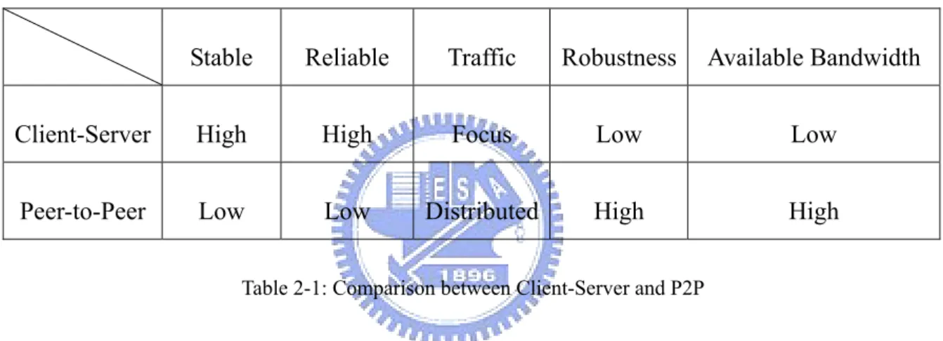
Summarize the advantages and disadvantages of client-server and peer-to-peer architecture. Table 2-1 shows the comparison between client-server and peer-to-peer architecture.

Table 2-1: Comparison between Client-Server and P2P

Client-server is more stable and reliable than peer-to-peer architecture. This is because data always store on single or multiple servers and service providers just keep server side working normal all time. To maintain small number of servers is much easy. That is why client-server architecture could provide stable and reliable service.

However, peer’s natural high churn makes the stability and reliability rely on all participating peers’ effort. It’s hard to make stable and reliable compared with client-server architecture. But the issue still could be alleviated by the well designed peer-to-peer architecture protocol.

Peer-to-peer architecture has overwhelming advantages in traffic, robust and available bandwidth aspects. Traffic in client-server structure usually is focus on the

Stable Reliable Traffic Robustness Available Bandwidth

Client-Server High High Focus Low Low

path toward server but peer-to-peer architecture distributed the traffic on the network topology. This is said that traffic distributed on the path in whole participants.

Robust in peer-to-peer structure is better than client–server structure because client-server architecture will end the service while the server is broken. Peer-to-peer architecture will stop the service while there are no participants in system.

Finally the available bandwidth in client-server architecture will decrease with the increasing of participants. But, the available bandwidth will increase in peer-to-peer architecture while the participants contribute more than its download bandwidth. So each peer under the restricted bandwidth can provide service for infinite peers.

Due to our objective, design a network structure fitted lived streaming, we choose peer-to-peer architecture as our network structure. Next section will introduce the related pee-to-peer researches.

2.2 Peer-to-Peer Structure Model

Peer-to-peer structure has three main models: tree, mesh and cluster. We will give each a brief introduction and compare three models.

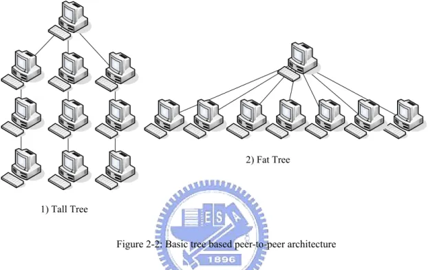
2.2.1 Tree Based Model

Peers connect to each other and form a tree which means that a peer has only one parent and one or more children. Figure 2-2 shows the two basic tree based

peer-to-peer architectures. Tall tree [15] [16] construction has least waste of available bandwidth but last few nodes will suffer from long delay. Each node in fat tree [17] has small delay but parents have relative heavy burden. However both of these methods can’t resist the transient behavior of peers. Moreover a tree based system

model needs a centralize mechanism to maintain peers’ position in a tree. A

peer-to-peer system should get rid of the centralize mechanism because huge crowd of peers might crash the central server.

2) Fat Tree

1) Tall Tree

Figure 2-2: Basic tree based peer-to-peer architecture

Maintaining tree based model needs less effort. However, it loses the distributed and robust advantages of a peer-to-peer system. It can’t solve the problem of high transient behavior. But it can deal with the heterogeneous channel conditions by optimally arranging peers in a tree.

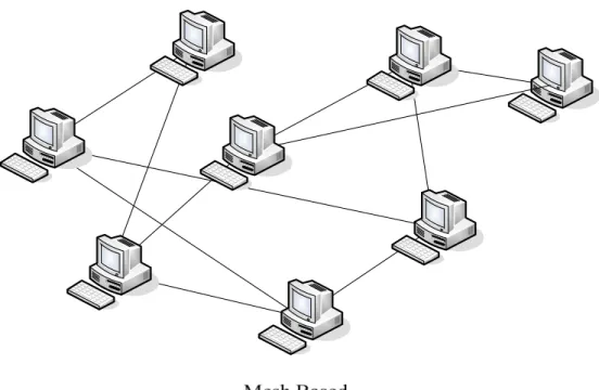
2.2.2 Mesh Based model

Mesh based model is a fully distributed system. [1] [7] use mesh based construction method. Peers gossip to its neighbors and acquire the overlay information without centralize mechanism. Figure 2-3 is an overlay example of a possible peer-to-peer mesh network.

Figure 2-3: Basic mesh based peer-to-peer architecture

However, mesh based architecture needs a complex protocol and a large number control messages. So, to maintain a mesh based network is not an easy job. Mesh based peer-to-peer network can’t immediately reflect the network situation to all participants. Peer might only get the information after few rounds of gossip. But the fully distributed characteristic can solve the heavy burden on servers or on few key peers in a tree based. This will enhance system robustness.

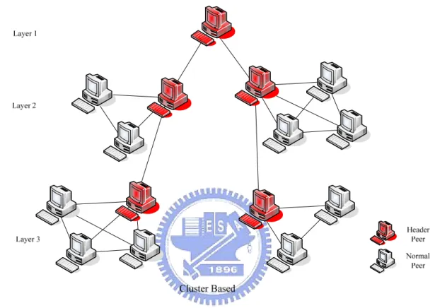
2.2.3 Cluster Based Model

A cluster based peer-to-peer architecture tries to combine the advantages in tree and mesh model. [18] [19] [20] use cluster method. In a cluster based peer-to-peer structure, peers will be divided into several groups by some factors. And then a cluster needs to pick up a leader. All group leaders form a tree based structure. Inside a cluster, peers form a mesh based structure. But the communication between peers in

different clusters must get through their leader (header). Figure 2-4 shows the simplest cluster peer-to-peer architecture. Header peer (Red) can cross layer communication and they construct like a tree. Normal peer just receives and transfers data in its group.

Figure 2-4: Cluster based

A cluster based peer-to-peer architecture is more robust than a tree based structure, and it has less complexity to construct the protocol than mesh based structure. But, forming a cluster still needs a centralize mechanism. Also we can’t promise the leader’s stability in a peer-to-peer system. So, cluster based structure didn’t solve the problem of transient behavior, it just leaves the problem to cluster leaders.

2.2.4 Comparison

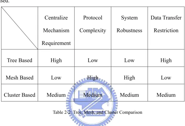
We summarize the advantages and disadvantages of these three construction models. Table 2-2 shows the comparison between tree based, mesh based and cluster based. Centralize Mechanism Requirement Protocol Complexity System Robustness Data Transfer Restriction

Tree Based High Low Low High

Mesh Based Low High High Low

Cluster Based Medium Medium Medium Medium

Table 2-2: Tree, Mesh, and Cluster Comparison

Tree and cluster structures rely heavily on the centralize mechanism. The centralize machine needs to record whole overlay connection and each peer’s state. And then central machine uses the algorithm to calculate the best peer arrangement location on the overlay. Mesh based still needs a central mechanism. This is similar to the tracker file for a new join peer. The central machine just replies a random peer list to the new comer. Then peer starts protocol to find parents. Due to the algorithm runs on each peer, centralized mechanism is much lighter in mesh based than others.

Tree based has lower protocol complexity. This is because central mechanism holds the overlay construction job. Peer seems to have an agent (central machine) which handles peer’s connection issue. Cluster based is more complex than tree based. This is because cluster leaders share the central machine’s burden. A cluster leader

manages its cluster works. The complexity of the mesh-based peer-to-peer architecture is the highest. In order to maintain the system, peer needs to gather parent, children, and data information. In a mesh based structure, fully distributed, peer should do those complexity jobs all the time.

Tree and cluster based structure is less robust. This is because they rely on specific peers such as single parent or cluster leaders. It’s hard to prevent the system form crashing while facing a high churn situation. Mesh based could totally resist the high churn problem. A peer connects to parents on its own. Also all peers are equal essential. The high churn couldn’t influence the mesh based architecture.

Data transfer shouldn’t be restricted by the overlay construction. Tree and cluster have the restriction due to their overlay construction. Mesh based structure can arbitrarily transfer data to each other. This is because a peer finds its parents on its own. Data transfer in mesh based structure is easier than in tree and cluster based.

We think mesh based is the best peer-to-peer structure model. It preserves the distributed and robust advantages of peer-to-peer system. Although mesh based model require a complex protocol design, personal computer today can alleviate the problem. Other two construction models didn’t preserve peer-to-peer advantages, therefore they are not suitable for our objective service, live streaming. In next section we will introduce solutions to the natural drawbacks of peer-to-peer architecture in literature.

2.3 Peer Fluctuation

File sharing is the well known peer-to-peer application. The natural drawbacks of peer-to-peer didn’t stand out in file sharing. This is because file sharing always considers the completeness of data receiving. Huge crowd of peers could recover the

influence of transient peers. Therefore, file sharing service is much suitable for peer-to-peer architecture. However, the issue of transient peers in streaming service can’t be covered by huge crowd of peers. This is because streaming service is fully time-dependent. Also, all peers require a stable streaming bit rate. High transient of peers and heterogeneous available bandwidth make the stability and delay fluctuation in a streaming system. This is the fatal drawbacks of streaming service on peer-to-peer architecture.

Fortunately, there are two ways to solve the peer fluctuation problem. One is the construction method of a peer-to-peer system, and the other is the streaming data protection. Error recover property existed in many coding techniques. For example, Forward Error-Correction coding (FEC) promises that receiving fix number of different encoded blocks can restore the original data content. Multiple Description Code (MDC) divide data into small groups. Receiver can restore low resolution of video content as long as it received one description. The more description it received, the higher resolution of video content it can watch. CoopNet [21] uses MDC to alleviate the damage of transient peers. On system construction side, CoopNet use multiple, diverse distribution trees transfer extra data to prevent the influence of overlay broken. However, without restriction of redundant data transferring will increase network burden. Also, there is a centralize tree construction mechanism. We think tree based peer-to-peer architecture can’t resist the high churn behaviors of peers. ROST [10] constructs an application multicast tree using the peer’s lifetime characteristic. The measurement of a peer’s ability in ROST is based on the product of bandwidth and lifetime (BTP). Because, they use the characteristic that peer who lives in system longer will have lower probability to leave the system. When a new comer in ROST, it will be placed at leaf. Then, it will exchange the position with its parent if

its BTP is bigger than its parent. Eventually, older peer will close to the root. The whole system will drive to stable because of the churn behaviors often appeared far from root. However, peer bandwidth and its lifetime have no relation. A new comer with huge bandwidth will close to root after a small period of time. This situation might make ROST unstable. Although ROST uses peer lifetime characteristic to achieve stability, tree based architecture isn’t fit into the scalability of peer-to-peer system. To make a peer-to-peer system robust, we shouldn’t rely on specific peers.

2.4 Peer Synchronization

Peer synchronization issue in peer-to-peer live streaming system is much important. We use popular peer-to-peer live streaming system [35] [36] which suffer from 30 to 300 seconds end-to-end delay. To decrease delay relies on peer-to-peer construction strategy. By constructing a short tree, [17] achieves the shortest path on an overlay. And this can enhance synchronization of all peers. [22] [23] make peer synchronize by considering the corresponding of physical network topology and overlay network. This consideration let transfer messages on overlay won’t have extra time consuming. However, to understand the network topology and routing are not an easy job. Except the observation method, rstream [24] uses mathematic induction to minimize the end-to-end streaming delay.

rStream formulates the small delay and bit rate satisfaction as a linear optimization problem. According to each overlay link delay and capacity, rStream decides upstream peer’s rate allocation with minimal delay. rStream on some aspects need central control mechanism. That is under a high churn situation peer will do update process at the same time. This burst throughput might be the miscalculating

2.5 Peer-to-Peer Network Maintenance

Peer-to-peer streaming protocol can generally classify into server driven, receiver driven, and data driven [25]. Server driven [26] [27] [28] is the tree based structure which root is data source. On the contrary, receiver driven is the tree based architecture which receiver is the root. Data-driven [1] [29] (gossip based) is that peer random selected its neighbors and peer exchanged information of others by many control messages (gossip). However, centralized algorithms usually need a power server to be root. This is hard to be a scalable streaming system. Therefore, many distributed algorithms try to solve this problem. ZIGZAG [19] minimize the transmission delay, and Splite-Stream [28] maintain multiple distributed tree to reach scalability.

CoolStreaming [1] is a data driven method also a mesh based structure. Peer in CoolStreaming have many partners. It used membership management and partnership management to retrieve the information of partners. Data coordination in multi-parents is important. To avoid redundant data, peers exchange data chunk availability using buffer maps. To exchange frequently buffer map and requesting specific data chunks will increase the amount of control messages. This is the disadvantage of a mesh based structure. Rateless code can solve the data coordination problem. We will introduce in section 3-2.

To maintain a peer-to-peer streaming system, tree based is simpler than mesh based. But, tree-based system always needs a power-server. It is not a scalable solution to a streaming service. We should use mesh based peer-to-peer system structure to make a scalable streaming service.

Chapter 3 Proposed Method

3.1 Preface

High fluctuation of node’s participation and limited bandwidth availability are the natural disadvantages of peer-to-peer network. As previous chapters describe, we know that to design a good lived streaming system should need a mesh based peer-to-peer network structure. rStream uses linear optimization model to design an efficient distributed optimal rate allocation algorithm and minimizes end-to-end delays. Moreover, rStream takes Luby Transform (LT) codes on data transformation. This code can reduce the amount of control messages for data reconciliation. However, rStream still has some drawbacks. 1) It still uses centralize mechanism when a joined peer does first optimal parent combination. 2) It takes passive measure while facing the transient of peer. When central mechanism finds many requests of rate recalculation, it sends broadcast messages asking all peers to rearrange its rate. 3) It takes advantage of pull-push data transfer scheme but they don’t consider the round-trip-time overhead of this scheme. 4) They have restriction of data transfer. A peer only can transfer the decoded data section.

Our proposed method makes peer exchange messages with others. Then, peer joins into the streaming system. We promise the stability of sufficient streaming data bit rate. In high churn surroundings, peer can calculate the lost probability of their parents. Thus, a peer will not be affected by the transient behavior of peers. Besides, we use effective throughput prediction to reduce the overdue data of pull-push data transform scheme.

Sub-chapters below are the details of our propose streaming system. It contains our proposed protocol, data transfer scheme, lifetime distribution, and other small issues of design this system.

3.2 Proposed Protocol

How to pick up a group of parents is the main part of a peer-to-peer protocol. Our proposed protocol is aimed at recovering the natural drawbacks of peer-to-peer architecture.

3.2.1 Parent Selection

Our parent selection algorithm uses lifetime distribution of peers and weighted factors to evaluate the ability of peers.

There exists a phenomenon in a peer-to-peer system. That is “the longer a peer lives in the system, the less probability it will leave later.” Also, this peer lifetime distribution can be modeled by heavy-tailed distribution [2] [4] [10]. (Most of researches use Shifted Pareto Distribution [30]) We use this distribution precisely point out the peer, i, reliable level Li(t) with its lifetime t.

We use three factors to measure a peer’s ability. These parameters use weighted adjustment. The three factors are PABW (Path Available Bandwidth), FL (Fresh Level), and ER (Effective Ratio). PABW is the probably upload bandwidth of a peer. FL represents the data latency of a node owning. ER shows the data usability of a node owning.

A. Path Available Bandwidth (PABW)：

calculates the PABW value itself, it sums up the PABW values multiply the reliable level L(t) of each parent of itself. (1). SPABW(i) represents the total bandwidth that a peer, i, will receive from its parents in the future. Later, a peer, i, compares this value (SPABW(i)) with its available bandwidth multiply its leaving probability D(t). Choose the minimum one as its PABW value (2).

Therefore, PABW factor represents the minimum supply bandwidth of a peer in the future. PABW factor on source is equal to the supply bandwidth of the child.

B. Fresh Level (FL)：

Fresh level (FL) represents the delay relative to the source node of a peer. The source must give a time stamp on the data packet. When a peer received data from its parent, it can realize the delay relative to the source. The fresh level value of a parent can be calculated by using the time stamp from source. The detail of fresh level calculation is that peer records all fresh level parameters of its parents. The peer chooses the maximal one from its parents as its fresh level parameter.

Fresh level parameter also shows data new/old level of a peer. If delay on leaf peers were as close as those peers who connected with source in a real time streaming system, peer-to-peer system can work more effective.

C. Effective Ratio(ER)：

Effective ratio is trying to show the data usability of a peer transmission. It is

∑

∈

×

=

sParent i j j j

t

L

j

PABW

i

SPABW

'

))

(

)

(

(

)

(

(1)

))

(

)

(

),

(

min(

)

(

i

SPABW

i

ABW

i

D

i

t

i

PABW

=

×

(2)

the parent. Above two factors predict the ability of a peer. This parameter can reflect the real contribution of a parent. Multi-parent scheme cannot avoid the waste of data generation and transmission. Besides reflecting the contribution of a parent, this parameter can restrain some parents from transferring redundant or overdue data. To compute this factor, a peer needs to receive a period of time data. The factor could be counted while the peer is already my parent. We will introduce the way to calculate this factor later (In 3.3.3). It has to combine with our data management model.

The evaluation score (ES) of a parent candidate Pi can be expressed as:

)

(

*

)

(

)

(

)

(

i

w

₁

FL

i

w

₂

PABW

i

w

₃

ER

i

ES

=

∗

+

∗

+

(

3

)

where w1, w2, and w3, are weighting factors.

The weightings of evaluation processes are set according to the factors leverage. Path available bandwidth factor can reflect a peer’s stability on data supply. Fresh level factor can reflect a peer owning data latency and closing to the source. Effective ratio shows the healthy level of data supply of a peer. All peers in a live streaming system hope to receive streaming data smoothly before leaving. We will enhance the weighting on PABW to keep receiving stable streaming data. ER still needs to consider, because it can reflect the streaming data usability. Also, we can’t ignore the latency of data, because in a live time streaming system overdue data is useless.

Finally, the new comer chooses the parents according to their evaluation scores. The number of selected parents depends on the summation of the evaluation scores of selected parents.

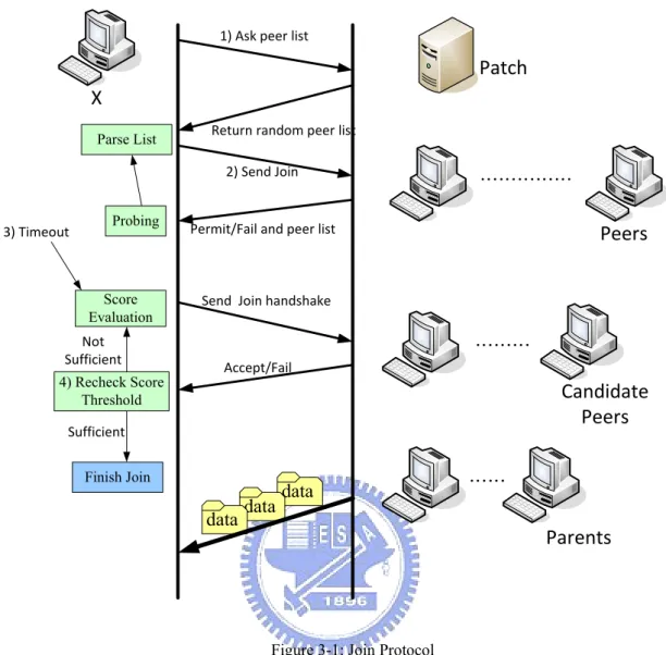
3.2.2 Join Protocol

We use four-way join protocol:

1) Peer X joins into the streaming system. Peer X asks a random peer list from a patch server. This server records partial active peers in the streaming system. When the server receives a request from a peer, it just replies randomly a list of peers.

2) Peer X sends out join message to all the peers who are on the list. Also, it asks them to reply another peer list which they connected with and the evaluation factors.

3) Peer X acquires information of other peers in a period of time. Then, it does the evaluation score process which we introduce above. Finally, it ranks the score and decides candidate peers. It sends out the join handshake message to those candidate peers.

4) Peer X receives accept/refuse message from candidate peers. When the summation of evaluation values of parents is exceed the threshold, peer X stops sending out join handshake message and it finishes the join process.

X Patch 1) Ask peer list Return random peer list 2) Send Join i Permit/Fail and peer list ……… Send  Join handshake Ci Accept/Fail Not  Sufficient Count Peers＇ 3) Timeout P Sufficient Peers i …… Parents i ……… Candidate  Peers data data data Parse List Finish Join 4) Recheck Score Threshold Score Evaluation Probing

Figure 3-1: Join Protocol

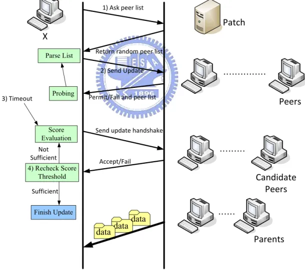
3.2.3 Update Protocol

Parents of a peer will leave the system arbitrarily. Peers should do update procedure to keep the stability. A peer checks the statuses of its parents in a fixed period of time. If parents are less stable or supply lower quality of data, a peer will do the update process. This represents that some of parents does not fit into the requirement of the peer. Thus, they should be replaced.

Update protocol:

server.

2) Peer X sends out update messages to peers who are on the returning peer list or connected with peer X. It asks these peers to return a peer list they

connected with and the evaluation factors.

3) Peer X acquires information after a period of time. Then, peer X does the evaluation score process which we introduce above. Finally, it ranks the score and decides candidate peers. It sends out the update handshake message to candidate peers.

4) Peer X receives accept/refuse message from candidate peers. When the summation of evaluation values of parents is exceed the threshold, peer X stops sending out update handshake message and it finishes the update process. X Patch 1) Ask peer list Return random peer list 2) Send Update i Permit/Fail and peer list ……… Send update handshake Ci Accept/Fail Not  Sufficient Count Peers＇ 3) Timeout P Sufficient Peers i …… Parents i ……… Candidate  Peers data data data Parse List Finish Update 4) Recheck Score Threshold Score Evaluation Probing

Through peer periodically does update process, our peer-to-peer system won’t be affected by the fluctuation of node’s participation.

3.3 Data Management Model

This sub chapter introduces our proposed data management model. It contains the data encoder, data decoder, data transfer protocol, score adjustment mechanism, and request rate allocation function.

How to construct a peer-to-peer system efficiently is a huge issue. Then, how to control data transferring between peers especially in multi-parents structure is also an important part. This is because peer exchanging data status can reduce to receive repeated or overdue data. Moreover, peer-to-peer system can reach the optimal utilization. However, too many data control messages are the redundancy. We use Luby transform codes [14] to reduce the data control messages between peers and the system performance can keep well.

3.3.1 Luby Transform (LT) Codes

Luby Transform Codes is one of rateless fountain codes. Rateless fountain codes includes LT codes [14], Raptor codes [31], and On Line code [32]. Rateless code is much suitable for peer-to-peer streaming data. The spirit of rateless code is that it can generate infinite coded data by finite messages. When receiver gets (1+ε)× N coded data (blocks), it can restore the original messages in a high probability. (N: number of original data, ε: a constant close to zero)

3.3.2 Luby Transform Codes Coding Scheme

The coding scheme of LT codes in our streaming system contains four parts. We will give an overview of coded flow of LT codes. Then, we will show the encoder and decoder of LT codes. And, following is the section based LT codes. The last is recoding benefit.

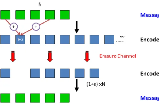
y Overview

LT codes uses XOR○+ operation to generate infinite coded data. First, it divides

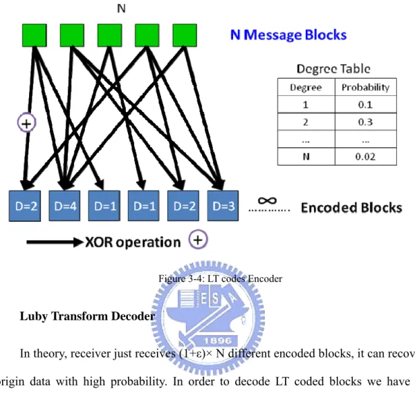
the transferred file into message blocks (N) with fix size. When generating an encoded block, LT codes uses a degree distribution to decide the degree (D) of this encoded block. Degree (D) means that to pick up number of D message blocks does XOR operation. Next, this encoded block picks up number of D message blocks randomly. This is the formation of an encoded block. Figure 3-3 shows the flow of LT codes. The second encoded block (blue) whose D is equal to 2 chooses randomly two message blocks (green) to do XOR operation.

Therefore, if we wanted to restore an encoded block, we should have the same degree distribution and random number generation system. Fortunately, this is easily fulfilled in present computer system.

Figure 3-3: LT codes flow

y Luby Transform Encoder

Luby transform encoder encodes files to infinite encoded blocks. It divides a file into fixed size message blocks (N). Numbers of message blocks (N) will influence the total amount of encoded blocks (4). Large of N will generate nearly infinite encoded blocks.

∑

=

=

N m N m

C

k

EncodeBloc

0

#

(

4

)

where N is number of message blocks.

The key of generating encoded blocks is the degree distribution. There are Ideal Soliton distribution and Robust Soliton distribution mentioned in Luby Transform literature. The probability degree distribution decides the degree D of an encoding block. It selects randomly D non-repeated message blocks to form an encoded block. Figure 3-4 is the process of generating encoded blocks. Each Æ represents an XOR operation. For example, the first encoded block is the first and the forth message

blocks do XOR operation.

Figure 3-4: LT codes Encoder

y Luby Transform Decoder

In theory, receiver just receives (1+ε)× N different encoded blocks, it can recover origin data with high probability. In order to decode LT coded blocks we have to construct the same relationship between encoded and message blocks in encoder.

When sender transfers an encoded block, it has to attach the information about how to generate this encoded block. Because the same random number generator and degree distribution are on every node, sender just attaches the random seed as the relative information. Decoder side can get the same relationship between message and encoded blocks. Figure 3-4 and 3-5.

Figure 3-5: LT codes Decoder

Decoding procedure keeps finding the degree one encoded blocks. Because encoded block with degree one is generated by one message block. In other words, the message block is equal to the encoded block Figure 3-6(a). The message block with degree one has been restored. While doing above procedure repeatedly, we can find some degree two blocks restorable. Because of one of message blocks which it connected with has been restored. After XOR operation, this encoded block with degree two decreases its degree to one. So another message block can be restored Figure 3-6 (b). In the end, we can restore all message blocks.

(a)

(b)

y Section Based LT codes

LT codes uses in file transport originally. But our objective is streaming, we have to do some modification on the data segmentation of LT codes. Figure 3-7 shows the transformation of LT codes from file application to streaming. We consider the streaming data as the target bit rate multiply a fix period of time. The production is equal to a small file. Therefore, we can use the benefit of LT codes without huge scale change.

LT decoders are independent on different time section, because each time section can view as a small file. Streaming application by using LT codes means many small files transfer with time restriction.

Figure 3-7: Section Based LT Codes

y Benefit of LT Codes

The reason we use LT codes is that it can reduce the data control messages. The natural characteristic of LT codes can totally solve the data control message overhead problem. Because any peer can generate infinity encoded blocks after decoding the streaming section data. Not only the source but all participants who decoded the streaming section have the ability generating different encoded block of this section.

reconciliation mechanism. With the help of LT codes characteristic, we can reduce the data control messages between parents and children. Also, it can simplify the data transfer protocol design.

3.3.3 Data Transfer Protocol

We use LT codes to simplify the data transfer protocol design. Also, we use section based data transfer scheme. A peer decides the start section after join or update procedure. The policy is that a peer picks up the start section which is all its parents receiving at most now. After a parent gets the message of section request, it transfers the section data to this child until receiving the next section request. Figure 3-8 is the data transfer protocol.

The measurement of effective ratio (ER) starts after decoding a data section. (Effective ratio mentioned in 3.2.1.) When a peer receives an encoded data packet from its parent, it can check this packet is useful or redundant. After decoding a section, a peer can easily count out the effective rate of their parents during last streaming section. This is said that peers can understand the contribution of each parent. The effective ratio of parents could be calculated by the ratio of the contribution to the data request rate of the parent.

Data receiving buffer is important for any streaming system especially peer-to-peer streaming system. It can relieve the damage of fluctuation of peers and different network conditions. A peer can receive a range of streaming sections, typically from the next section of playback to a small number of future sections. Also, peers need to transfer streaming data in a peer-to-peer system. They should have data sending buffer. Data sending buffer should not be too large in a real time streaming

system because of the time limitation. Our purposed streaming system uses small (two) sending and receiving section buffers.

Parent B

Parent A

Child

Request Sectio_{n i} Section i d ata Section i d ata Section i d ata Section i d ata Section i dat a Section i dat a Section i dat a Decoded

Section i _{Request Sec}

tion i+1 Section i+ 1 data Section i+ 1 data Section i+ 1 data . . . . . . . . . Star Section Selection Section i d ata Request _{Section i} Reques_{t Sectio} n i+1 ER calculation

Figure 3-8: Data Transfer Protocol

3.3.4 Request Rate Allocation Function

This function allocates the request rate to each parent. The request rate RequestRate(i) to a selected parent, i, is according to the parent’s evaluation score as shown in (5).

Rate MAXRequest j ES i ES i e RequestRat Parents j × =

∑

∈ ) ( ) ( ) (

(

5

)

We request higher rate to those peers with higher evaluation value, because the evaluation score of a peer represents its ability. We restrain the transfer rate of parents with low score and enhance the others. This adjustment of request rate will make our system more robust to different network surroundings.

3.3.5 Score Adjustment Mechanism

A parent might not be able to fulfill the request rate from its children due to the constrained upload bandwidth of the parent. Our rate allocation function depends on parent’s evaluation score. Therefore, the evaluation score of a parent needs to update frequently. Then, it can rapidly reflect the statuses of parents. We call this mechanism score adjustment.

Score adjustment is triggered after effective ratio calculation. We use the moving average αi of effective ratio to adjust the score of peer, i, as shown in (6) and (7). As a result, the evaluation score of the parent who suffers from insufficient upload bandwidth will decrease, as well as the importance of this parent to the peer.

)

(

8

.

0

2

.

0

_i

ER

i

i

=

×

α

+

×

α

(

6

)

i

i

ES

i

ES

(

)

=

(

)

×

α

(

7

)

3.4 Peer Lifetime Distribution

3.4.1 Lifetime Distribution Research

Peer lifetime distribution is a possible solution for the fluctuation behavior of peers. Many researches analyze possible behavior of peers by observing a peer-to-peer system over a long period time. Most of the results show that peer lifetime distribution can use heavy-tailed distribution to approximate. Besides, the characteristic is “the elder peer has smaller probability to leave system than younger peer.” Some researches take advantage of this characteristic on their parent selection algorithms. Pareto distribution is one of the heavy-tailed distributions. In [30] [33] use shifted Pareto distribution (8) to model lifetime duration of a peer.

0 , 0 , 1 , : 1 ) ( ) 1 ( > > > ⎟⎟ ⎠ ⎞ ⎜⎜ ⎝ ⎛ + = − − x where x x f

α

β

β

β

α

α ₍₈₎

3.4.2 Continuous to Discrete Lifetime Distribution

We use shifted Pareto distribution to model the lifetime of a peer. But, shifted Pareto distribution is a continuous probability distribution. We have to modify it to fit into our system. This is because a digital system cannot use continuous function. Sampling is the way to change a continuous distribution into a discrete one. After sampling shifted Pareto distribution, we should make sure that it still has heavy-tailed property.

distribution every s seconds as shown in (9).

N

i

where

is

s

i

x

x

x

d

x

dx

x

dx

x

dx

x

dx

x

dx

x

dx

x

f

x

P

N

i

s

i

x

is s i is s i is s i is s i is s i is s i is s i is s i is s i

∈

>

>

+

−

−

+

=

+

−

=

+

−

=

+

+

=

+

=

+

=

⎟⎟

⎠

⎞

⎜⎜

⎝

⎛

+

=

⎟⎟

⎠

⎞

⎜⎜

⎝

⎛ +

=

⎟⎟

⎠

⎞

⎜⎜

⎝

⎛

+

=

=

∈

×

=

− − − − − − − − − − + + − + + − + − − − − − − −

∫

∫

∫

∫

∫

∫

∫

,

0

,

1

,

]

)

(

)

)

1

(

[(

]

)

(

[

]

)

(

1

[

)

(

)

(

)

(

1

)

(

1

)

(

)

(

) 1 ( ) 1 ( ) 1 ( 1 ) 1 ( 1 1 ) 1 ( 1 1 ) 1 ( 1 ) 1 ( ) 1 ( ) 1 ( ) 1 ( ) 1 (

β

α

β

β

β

β

β

β

α

αβ

β

β

αβ

β

β

αβ

β

β

β

α

β

β

β

α

β

β

β

α

β

β

α

α α α α α α α α α α α α α α α α (9) Next, we need to verify P(x) is a probability distribution.

1) Probability value shouldn’t be negative. (10)

0

]

)

(

)

)

1

(

[(

)

(

0

,

0

)

(

)

)

1

(

(

0

)

(

)

)

1

(

(

)

(

)

)

1

(

(

)

(

)

)

1

(

(

0

,

,

,

)

(

)

1

(

]

)

(

)

)

1

(

[(

)

(

≥

+

−

−

+

=

∴

>

∞

→

=

+

−

−

+

>

+

−

−

+

∴

+

>

−

+

∴

+

<

−

+

∴

>

+

<

−

+

+

−

−

+

=

− − − − − − − − − − α α α α α α α α α α α α α α α

β

β

β

β

β

β

β

β

β

β

β

β

β

β

β

β

β

β

is

s

i

x

P

i

where

is

s

i

is

s

i

is

s

i

is

s

i

s

i

where

is

s

i

is

s

i

x

P

Q

Q

(10)

1

]

[

)

2

(

)

(

)

(

[

]

)

(

)

)

1

(

[(

]

)

(

)

)

1

(

[(

)

(

]

)

(

)

)

1

(

[(

)

(

1 1 1

=

=

+

−

+

+

+

−

=

+

−

−

+

=

+

−

−

+

=

+

−

−

+

=

− − − − − ∞ = − − ∞ = − − ∞ = − −

∑

∑

∑

α α α α α α α α α α α α α α α α

β

β

β

β

β

β

β

β

β

β

β

β

β

β

β

β

K

s

s

s

is

s

i

is

s

i

x

P

is

s

i

x

P

i i i (11)

So we have verified P(x) is a probability distribution. Now, we will make sure P(x) still has the heavy-tailed property. A distribution is said to be heavy-tailed if:

,

0

,

]

[

X

>

x

≈

cx

−

x

>

P

α

where 0 < α < 2 and c > 0 are constants. We prove the heavy-tailed property on discrete shifted Pareto distribution as shown in (12).

α α α α α α α α α α α α α α α α α

β

β

β

β

β

β

β

β

β

β

β

β

β

β

β

− − − − − − − ∞ = − − ∞ = − − ∞

=

≈

−

+

=

+

+

−

+

+

+

−

−

+

=

+

−

−

+

=

+

−

−

+

=

=

=

>

∑

∑

∑

x

js

s

j

s

j

js

js

s

j

is

s

i

is

s

i

js

x

where

x

P

x

X

P

j i j i X

)

(

]

)

)

1

(

[(

)

)

1

(

(

)

(

)

(

)

)

1

(

[(

]

)

(

)

)

1

(

[(

]

)

(

)

)

1

(

[(

,

)

(

)

(

K

(12)

distribution and a peer lifetime distribution. Then, we can calculate the leaving probability D(t) of a participant after it survived time period t.

Our parent selection algorithm can calculate more precise reliable level of a peer with this information. We argue that parent selection algorithm combined with peer lifetime distribution could effectively control the fluctuation of peers.

3.4.3 Residual Lifetime Expectation

To count the reliable level of a peer needs the residual lifetime expectation of a peer. First, we introduce the residual lifetime expectation. Residual lifetime expectation R(x|x>t) means how long a peer will survive after it lived t seconds as shown in (13).

t

t

x

P

x

P

x

t

t

x

P

x

P

x

t

t

x

x

E

t

x

x

R

t t

−

≤

−

⋅

−

=

−

>

⋅

=

−

>

=

>

∑

∑

∞ +

)

(

1

)

(

)

(

)

(

)

|

(

)

|

(

0 1

μ

₍₁₃₎

:where E(x|x>t) is the conditional expectation of t and μ is mean of P(x).

So, we define the reliable level L(t) of a peer is that the probability of a peer who will keep survive until I (peer) leave the system as shown in (14).

)

(

1

)

(

1

)

(

)

(

)

|

(

)

(

t

x

P

t

B

x

P

t

x

P

t

B

x

P

t

x

t

B

x

P

t

L

≤

−

+

≤

−

=

>

+

>

=

>

+

>

=

(14)

:where B is the residual lifetime expectation of a peer itself and t is the peer already survive time.

keep survive until I leave the system (B+t). Thus, we can measure the reliability of a peer.

3.4.4 Summary

We use discrete shifted Pareto distribution to model peer lifetime. Then, we are able to measure the reliability of a peer by calculating residual lifetime expectation of the peer. Reliable level L(t) represents the probability that a peer who already survived time t and it will keep in system until I leave. We combine this information to our parent selection algorithm. We make the path available bandwidth (PABW) evaluation factor more precise. This is said that we can measure the possible bandwidth that a parent will give to me in the future. Therefore, our parent selection algorithm could effectively control the fluctuation behavior of peers.

3.5 Other Detail Design

Except above main system structure description, some small issues will influence the whole system performance. These small issues are hot spot problem and data protocol overhead.

3.5.1 Hot Spot Problem

We say peer-to-peer system is high robust because all peers are equal essentials. If we rely on some specific peers, system performance will be unstable when those peers fail or leave. Tree based peer-to-peer construction is the best example. Our proposed method can distribute the importance of each peer by our multi-factors evaluation algorithm. Besides the evaluation algorithm, we design an active detect

mechanism to enhance the distribution of essentials of peers. This mechanism can achieve better system performance. According to our data protocol, we use section based data transportation. We adjust the scores of parents by its contribution after a peer decoded a section. Then, the new request bit rate of each parent is calculated according to the new evaluation score of the parent. We suppose a parent who can satisfy the request rate of a peer this section. The parent might satisfy more request rate next section. Therefore, a peer divides its parents into two groups before it request new bit rate. The policy of classification is the parent satisfied data request rate last section or not. If the parent cannot satisfy my data require bit rate last section, its next section request data bit rate will be limited in the require bit rate of last section.

Through this method, child can decrease the require bit rate from hot parent. We could make all participants more equal essentials, therefore our peer-to-peer system will be more robust.

3.5.2 Data Protocol Overhead

Our data transfer protocol might have some overdue data transmission. This situation happened during peer sends out next section request until it receives next section data. Figure 3-9 shows the overdue data transmission. The best way to solve this problem is that a peer sends next section request message in advance of a round trip time. This is because some of data blocks are in the network pipe. We can predict a round trip time effective data throughput by calculating the effective contribution of a parent from this section start to now. This small algorithm can reduce the overdue of our data transmission. We have simulation in chapter 4.6.

Figure 3-9: Data Protocol Overhead

3.6 Benefit of Our Peer-to-Peer System

One of the most important objectives of a peer-to-peer streaming system is to make peers receive stable streaming data. The characteristic of stable and reliable data receiving can make a peer catch up with the source playback rate faster and thus it helps to reduce the end-to-end streaming delay.

The proposed parent selection algorithm takes the upload bandwidth of a peer, among other factors, into consideration and we enhance this metric by combining with lifetime distribution of a peer. A peer can choose parents who are able to supply stable streaming data better over other peers.

The restriction of data transfer in rStream is that a peer can only send the data which it already decodes. The purpose of this restriction is to try to decrease data packets with high correlation between peers. This restriction will make the delay accumulate fast. The proposed data transfer protocol in this dissertation removes such restriction. A peer can start to serve its child peers once a section contains some coded blocks so as to reduce the difference of decoded sections between peers which will in turn enrich the list of parent candidates when a peer joins the system or performs the process of parent update. From the simulation results shown in Section 4, the proposed algorithm shows almost half of the end-to-end streaming delay reported in rStream [24]. To sum up, the proposed peer-to-peer streaming system consider multiple factors, including peer lifetime distribution and LT codes, besides the well-designed data transfer protocol. It can achieve small end-to-end streaming delay.

3.7 System Structure

Our system contain join, update protocol module, data management module, and peer list maintenance module. Figure 3-10 shows the system module details and the relation between each module. Peer list maintenance module contains parent selection module, evaluation score function, lifetime distribution, and peer list monitor. Data management module contains transfer rate allocation, request rate allocation section selection function, score adjustment module, parent contribution recording, data

Chapter 4 Simulation Result

4.1 Simulation Surroundings

In this chapter, we present results from experiments in simulated peer-to-peer streaming environments, based on our implementation of proposed system with the C++ programming language. The simulation platform is NS-2 2.29 and network topology is random generated with BRITE topology generator. Figure 4-1 is one of the topologies. We put our peers on the leaf and the middle nodes (core network) are generated by BRITE.

4.2 Parameter Setting

Pareto Sampling (s) 2 seconds

Peer upload/download capacity 1024 Kbps Source upload capacity 10 Mbps Join/Update Probing Time 1 second

Score Threshold 8

Update time period 5 seconds

LT block size 1024 Bytes

LT section size 128 K Bytes

Target bit rate 512 Kbps

Buffer size 2 sections

Simulation Time 1500 seconds

Table 4-1: Parameter Setup

4.3 Different Weight Setting

According to formula (3), we have to decide a better combination of weights. Due to the summation of three weights, we narrow the searching range on the plane of the equation w1+w2+w3=1. Then, we use the gravity of triangle to reach the better solution. Figure 4-2 is the gravity of triangle and the reaching process.

(0,1,0)

(0,0,1)

(1,0,0)

(1/3,1/3,1/3)

(2/3,1/6,1/6)

(1/6,1/6,2/3)

(1/6,2/3,1/6)

(1/3,7/12,1/12)

(1/12,7/12,1/3)

(1/12,10/12,1/12)

Red:Level-1

Blue:Level-2

(Fresh Level ,Path Available Bandwidth, Effective Ratio)

Figure 4-2 : Weight Setting Reaching Process

Each point is the gravity of each triangle and the weights from left to right is fresh level, path available bandwidth and effective ratio. Red points are the level-1 combination of weights. After the level-1 process, we run level-2 process from the best solution in level-1. In the end, we will find the best combination of weights.

We use three metrics to measure a combination of weights. They are the averages of effective throughput, the average of source section difference and the average of continuous index. The effective throughput of a peer is calculated by none repeated and in time Luby Transform data packets (encoded blocks) every two seconds. The

average of source section difference is the average of the section difference of all peers from source every 10 seconds. Finally, the continuous index is the playback smooth level. The way to calculate continuous index is the ratio of successful playback sections to whole sections in the lifetime of a peer.

Due to the time restriction, we only run to level-3. We get the better result under the combination of weights (1/6, 2/3, 1/6). The path available bandwidth is the most important factor. This is reasonable because when a peer did not have sufficient data bit rate, it cannot enjoy the streaming content even owning the latest data content. The other two factors: fresh level and effective ratio, we cannot distinguish the importance level under above combination of weights because they are the same. However, we can realize the different importance level while we observe the whole level-3 results. In our results, left level-3 point has better performance than right point. The fresh level is a little higher important than effective ratio. We believe that we can find the best combination of weights by using this gravity of triangle method, and the importance level of three weights is path available bandwidth > fresh level > effective ratio.

The weight setting in later simulation is (1/6, 2/3, 1/6) if no other explanation.

4.4 Synchronization of Peers

This experiment shows the average end-to-end streaming delay under different number of peers in system simultaneously. The media streaming bit rate is 300 Kbps and source has 10 Mbps upload capacity. We consider two classes of receivers: asymmetric digital subscriber (ADSL) and Ethernet peers. The ratio of two classes is 7 to 3. The download capacities of ADSL group are in the range of 512 Kbps ~ 3