TSS: a daily production target setting system for fabs

TSS: a Daily Production Target Setting System for Fabs]

Guan-Liang Wu, Kang Wei, Chih-Yang Tsai, Shi-Chung Chang Control and Decision Laboratory

Department of Electrical Engineering National Taiwan University, Taipei, Taiwan, R. 0 . C.

Email: scchang@,ac. ee. ntu. edu. tw

Nan-Jye Wang, Rong-Long Tsai, Huei-Ping Liu Taiwan Semiconductor Manufacturing Corporation

Hsin-Chu, Taiwan, R.O.C. MFG-2B

Abstract

In this paper, a Target Setting System (TSS) is designed as a computer aided decision support, which includes three modules: (1) Master Production Schedule Conversion (MPSC), (2) Capacity Estimation, and (3) Target Setting Main Function (TSMF). MPSC converts wafer release and output schedule into daily demanded moves of each production stage while CE estimates tool capacity by taking auto-regression of the actual move data. TSMF then takes the outputs of MPSC and CE and WIP distribution as its inputs, and adopts PULL, PUSH and iterative proportional capacity allocation schemes to calculate the daily target of each stage. TSS has been implemented for daily application. The scheduled total moves by TSS are within 5% of what have been actually achieved in the shop floor and about 50% of scheduled stage targets are within 15% difference with actual stage moves.

This work was supported in part by the National Science Council of the Republic of China and Taiwan Semiconductor Manufacturing Co. under Grants NSC 85-2622-E-002-018R and NSC 86-2622-E-002-025R.

1. Introduction

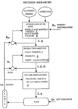
Functions of a decision hierarchy for target-based production flow control in a fab is depicted in Figure 1. Major issues include (1) wafer release and output scheduling, (2) daily target setting and (3) lot dispatching [2, 51 Wafer release/output aims at controlling the wafer-in-process (WIP) level and cycle time while meeting delivery requirements. It schedules the quantities of wafer release and output using a day as a time unit over two to four months. Lot dispatching determines which lot to process next when a tool is available. Daily target setting bridges between these two fbnctions. It combines daily release/output schedule, present fab production states, and tool capacity forecast to properly set daily production targets at each production stage, which then serves as a guideline for dispatching .

Operational complexity of a foundry fab is rooted in its high-variety, low-volume production and very complicated fabrication processes. There are typically multiple operation objectives for setting daily targets: (01) (02) (03) (04) (05)

to meet target monthly output volume, to balance the production line,

to reduce WIP and cycle time, to maximize tool utilization, and

to facilitate on-time delivery of products.

In addition, there are often time varying operation constraints and manually maintained data, which may not be completely captured by the manufacturing execution system (MES) due to very dynamic

and complex operations. Daily target setting is therefore quite challenging and a computer-aided decision support tool is highly desirable for daily operations.

In the past few years, Chang et a1 have developed a series of algorithms based on deterministic problem formulation for daily target generation and tool allocation (TGMA) of a foundry fab. The core method [ 11 of these algorithms adopts an iterative, proportional resource allocation approach that combines flow balance relationship, deterministic queueing analysis and some empirical rules to capture the important decision factors such as maximizing production moves, balancing the line, reducing WIP levels and prediction of detailed production flows. After the first successful field application at TSMC, the core method was extended to weekly short-term scheduling WTGMA) [6]

were implemented into tools and were applied in the field. method is also available [4].

Some theoretical analysis of the core

Although TGMA-based tools have achieved some successes, there are four major deficiencies that hindered the long lasting applications of these tools:

1)Exact numbers of tools at the beginning of a day are used in capacity calculation, which actually vary during the day and differ a lot from those taken for calculation;

2)Standard WIP of each stage requires empirical input and adjustment;

3)Standard processing times are used for production flow and cycle time calculation, which are difficult to be accurately maintained in a foundry fab of high product variety, low volume per product and frequent tool change;

4)Insufficient accuracy in capacity modeling of some critical tools.

Deficiencies 1) and 3) are due to unnecessary data accuracy requirements, which need not be so accurate for the purpose of daily target setting. Deficiencies 2) and 4) require a new algorithm and a detailed model respectively.

In this paper, we develop a new Target Setting System (TSS) as a computer decision-aid for setting the daily target of each production stage. TSS is designed by simplifying the data requirements and unnecessary algorithmic complications, enriching fhnctionality and enhancing user interface of the existing TGMA-based tools. It includes three major fkction modules: (1) Master Production Schedule Conversion (MPSC), (2) Capacity Estimation (CE), and (3) Target Setting Main Function

(TSMF). MPSC and CE hnctions are then described in

Section 3 and TSMF described in Section 4. Section 5 presents field test results. Finally, concluding remarks are summarized in Section 6.

Section 2 first gives a system overview.

11. System Overview

In addition to the five objectives (01-05) listed in the Introduction, TSS is also designed to

( 0 6 ) track higher level production targets;

(07) be able to estimate wafer flow-in and forecast WIP distribution;

(08) support dynamic calculation of standard WIP at each production stage;

(09) minimize requirements for manually maintained input data by modification of algorithm; and

(010) provide a friendly user interface.

evolves. However, the problem is very challenging because of the dynamic nature and complexity of a foundry fab.

To reduce the problem complexity and focus on the purpose of daily target setting, we make a few assumptions:

A l . A M P S is available, which is based on reasonable estimation of mid-term tool capacity and

production demands.

A2.

Detailed characteristics and constraints of tool operations are neglected; empirical statistics about tool capacity are used as aggregate characterization.

A3. There exists no priority difference among prodcuts A4. The production unit is a wafer

A5. The fabrication process of each part type is fixed.

A6. Stage is adopted as the basic unit for describing process flows, where a stage of a product type is obtained by aggregating a few consecutive fabrication steps of the product type.

A7. All the stages of various fabrication processes can be arranged into a global sequence of totally J

stages in a way that if stage k precedes a stage k’ in one process, the stage k also procedes stage k’ in the global stage sequence.

-, A8. Each stage has a corresponding key tool group. As steps of a stage may require tools from

different tool groups and different stage may also share the same amchine groups, the tool group that has the highest ratio of processing time over number of tools among the steps in a stage is selected to be the key tool of the stage.

A9. Buffer space is large and can be considered as infinite.

Figure 2 depicts the TSS system fbnctional flow chart. The MPSC module converts wafer release and output schedule of M P S into daily demanded moves of each production stage according to the average cycle time of each stage and the process flow of each product. It also recommends the reference WIP levels for next day production. As long as all daily demanded moves are achieved every day, on-time delivery of M P S demands can be accomplished and cycle time variation controlled. The

MPSC module is designed to run daily. The CE module estimates the capacity (number of wafer moves) of each tool type per day. It takes a moving average of the actual move data of individual tool over a certain period of time as the estimated capacity. And finally, TSMF takes daily stage demands from MPSC, tool capacity estimates from Capacity Estimation, and WIP distribution from the MES to calculate the daily target moves of each stage.

111. Demanded Move Calculation and Capacity Estimation

MPSC and CE modules correspond to higher levels in the decision hierarchy of production flow They set the environment of TSMF and significantly affect the accuracy of target setting. control.

The two hnction modules are now described respectively.

III. 1 MPSC Module

Inputs of the M P S C module are

- WIP levels by stage by part type,

- actual wafer output by type up to date,

- process flow of individual part types,

- cycle times by stage by type, and

-

M P S schedule (wafer start and output) for the coming three months,

which can all be obtained form the manufacturing execution system (MES) or the management information system(MIS). The outputs include

-

demanded numbers of wafer moves by stage by type during the day under consideration,

- delayed numbers of wafer moves by stage by type at the beginning of the day under consideration, each of which is the differences between the demanded and the actual cumulative moves to-date for a type at a stage, and

- the reference WIP levels by stage by type for next day production.

Let us now define some notations. As M P S C is designed for individual part types, the part type index is omitted in the following notational definitions.

Notations

J: total number of stages;

j : stage index, j=1, ,J, T: time horizon; t: time index, t= 1, . . . ,T; d: current time;

CT,: empirical cycle time of stage j , j=1 , . . . ,J, WIP,(t): empirical cycle time of stage j , j=l,. . .,J; MPS-OUT(t): the delivery quantity of day t in the M P S ;

QC-OUT(t). the delivery quantity of day t in the M P S ; DD,(t). demanded moves of stage j during day t ,

Cum-DD,(t): cumulative demanded moves from day 1 to the end of day t-1 at stage j;

MPS-day-demand,(d): total demanded moves of current day including DD,(t) and the delayed number of moves up to the end of t-1.

The MPSC algorithm converts, for each part type, wafer release and output schedule of M P S into demanded moves of each production stage. It is described as follows.

MPSC Algorithm

Step I : Compute, for all the M P S outputs, the available time of MPS-OUT(t) = t - d, t=l,. . .T.

Step 2: Compute the remaining cycle time from a stage j to output backward in stage sequence, RCT, = CT,,

RCT, = CT,

+

RCT,+l, for j=J-l,. . . , 1.

Step 3: Compute the slack times of individual stages,

SLJ = t

-

d

-

RCT,+I, forj=l,. . .,J.

Step 4 : Calculate the demands by M P S for the current day. The demand for stage j due to MPS-OUT(t), t=l, . . . ,T, is

x, O < x l l

MPS-OUT(t)* rI(SLJ), where

n(x)

=

1

2

-

x, if 1 < x I 2,

0, otherwise. Total demand by M P S for stage j is therefore

T

DDj (d) = xMPS-OUT(t)

*

Il(SLj), j = 1,. . ., J, t=l

and the cumulative demand up to the beginning of the current day is

d - - -1

CUIII-DD j (d) =

C

DD j (t), j E l,.. ., J.

t=l

Step 5: Calculate the demanded (to be fulfilled) moves by M P S for the current day

The cumulative moves of stage j that have been accomplished up to the beginning of the current day can be calculated by

J

Actual-move,(d)= z W I P j l ( d ) + QC-OUT(d), j =l,...,J,

j'= j+l

where QC-OUT(d) is the amount of output wafers up to the beginning of the current day. The demanded (to be fulfilled) moves by M P S for the current day is

MPS-day-demand .(d)=Max{DD.(d)-t Cum-DD.(d)-Actual-move.(d), 0), j = 1 , ..., J.

I J I J

LII.2 CE Module

Inputs of the CE module include

-

tool ID, type and stage mapping tables,

- multi-chamber tool ID table,

-

tool time data of the previous day such as up, lost, backup and hold times,

-

actual moves of the previous day,

-

capacity estimate for the previous day, and

- process flow of individual part types.

Let c,(t) be the capacity estimate of day t for tool group m and C,(t) be the auto-regression (AR) Previous day utilization of each tool is first calculated by utilizing the tool estimate for tool group m.

time data. The value of c,(t) is obtained by actual moves of tool k

utilization of tool k ' c"=

keM,

where the summation is over all the tools belongmg to tool group m.

then

The AR estimate for tool group m during day t is

C,(t)=ac,(t)+(l-a)C,(t-l), O I a 1 1 .

IV. Target Setting Main Function

Reference WIP levels are critical to target setting. In TSMF, the reference WIP level of a stage is set as the average WIP level under the M P S demanded moves of the next day, which can be calculated by applying Little's formula. Such a definition is intended to prepare for the next day operation through efforts of the current day A PULL procedure is first used to calculate the up-to-date cumulative production demand of each part at each stage. Tool capacity is allocated to such demands proportionally among individual stages[l] For the residual tool capacity and WIPs aRer PULL, a PUSH procedure then tries to push as many as possible residual WIPs of individual stages to their respective downstream stages so that the tool utilization can be maximized and cycle times can be reduced. Target moves of individual part types at a stage are obtained by adding up, across all part

types, the PULL targets and PUSH targets of the stage. Note that in the one hand, the available WIP of

individual stages affects the setting of reasonable targets; on the other hand, target settinghool allocation affects the flow-in from up-stream stages and hence available WIPs of individual stages. Cycle time statistics are also exploited to pose a heuristic constraint on updating the amount of flow-in

wafers to each stage. The maximum number of flow-in wafers for a stage is the sum of initial WIPs of upstream stages that are within one-day cycle time to the stage under consideration. The PULL,

PUSH and Flow-in updating procedures constitute an iteration of TSMF and are repeated till the calculated set of stage targets converge. Figure 1 gives the fknctional flow chart of TSMF.

To formalize the description of the algorithm, let us add the part type index to the previously defined notations and further define some new notations.

Notations

I:

i:

Tom-Dem,. daily M P S demand for type i at stage in the next day; WIP,. the WLP level of type-i parts at stage j at the beginning of the day; Ref-WIP,. the desirable WIP level preparing for next day production at stage j .

Flow- in,. number of type-i wafers flowing to stage-j from its up-stream stages during the day; R,:

M. m:

C,: S,:

total number of part types; part type index, i = 1,. . . I;

amount of type i wafer start for the day; the total number of tool groups;

the tool group index,m=l, . . ,M;

estimated capacity of a tool in group m in term of wafers per day;

the set of all part type and stage pair (i, j) that require tool group m for processing;

Decision Variable

Target,: number of type-i wafers leaving stage j to its down-stream stages.

TSMF Algorithm

Step 0: Initialization

Input all the necessary data.

Set Flowin,, = R for all i, and Flow-in = 0 for all i and j=2,. . . J

F o r i = 1, ..., I

Stepl: Compute the reference WIP levels. Ref-WIP, = Tom-Dem,* CT,, j = l , . . .,J

Step 2: Compute the maximum number of flow-in wafers to each stage,

Forj=J, J-1, ..., 2,

Max-flow

~,,

= 0,

j 7 = j ,

While Time < 24 hours and j > 1, j 7 = j 7 - 1 ,

Max-flow lJ, = Max-flow

',,

+ WIP

',.,

Time = Time

+

CT l,..

Pull Procedure

Step 3: Calculate the PULL demand for each stage by considering the demand of the stage itself, the downstream stage demand and the number of available WIP.

For j = l , . . . ,J

Pullf,, = Max (0, MPS-day-demand I@+l) -t R e f - m qk+i)

-

WIP I(k+i) >,

Pullf

',,

= Max (MPS-day-demand 1,, Pullf ,),

Pullf

',,

= Min (Flow-in ?1 + WTP ',,, Pullf,).

Step 4 : Allocate tool capacities by part type and by stage proportionally to their WIPs. For m=l , , . . ,M,

For each part type i that uses tool group m at stage j,

Pull,, =

Push Procedure

F o r i = 1, ..., I

Step 5: Calculate the remaining WIP of each stage that can be pushed to the down stream stages. For stages j = l , . . . ,J,

Push lJ = Max [0, Flow-in IJ

+

WIP I,

-

Pullf J .

Step 6: Allocate residual capacity of tools by part type and by stage proportionally to their remaining WIPS.

For each part type i that uses tool group m at stagej,

Step 7:Generate new targets and check convergence. Target, = P u l l ,

+

Push,, I=l, ..., 1, j=1, .,.,

J.

I J

If X z l T a r g e t i j -Flow-ini~+1)11@, then i=l j=1

Output Target, and Stop.

Step 8: Update Flow-in and iterate. Flow-in = Min ( Target

Go to Step 3 for the next iteration

, Maxflow 1, )

V. Implementation Results

In designing and implementing TSS, the desirable features include (1) meeting the production demands of M P S , ( 2 ) line balancing, (3) mean cycle time and variance reduction, (4) manual data maintenance reduction, (5) maximization of daily moves, (6) wafer flow-in forecast, and ( 7 ) target adjustment for banking and scrap. Table 5.1 summarizes the coverage of these features by individual TSS functions. Note that although the data files of key tool, tool subtype and its mapping to production stages require manual maintenance, they are maintained at a monthly or quarterly frequency.

TSS has been implemented for daily application Production supervisors briefly review and adjust the targets generated by TSS every morning. Targets are then delivered to shop floor after the production meeting There have been less then 20 out of a total of 140 production stage targets each day that require some adjustments. Figure 2(a) depicts that the scheduled total moves by TSS (before manual adjustments) are mostly within 5% of what were actually achieved in the shop floor Since

the daily capacity variation of tool is about 10 - 15% of the forcasted capacity, we consider the scheduled daily target of a stage accurate if it is within 15% of the actually achieved number of moves. The performance of TSS on stage target accuracy is given by Figure 2(b), which shows that about 50% of scheduled stage targets are accurate.

Detailed analyses indicate two potential cause of the by-stage inaccuracy of TSS. The first is the discrepancy between the demanded moves calculated from M P S and what are desired in a day by the shop floor managers. As TSS is driven by M P S , such an observation suggests hrther integration between M P S and shop floor scheduling in operational philosophy. The second is the use of empirical cycle times, which are very well known to be in accurate; they vary a lot from day to day with respect to actual WIP distribution and available tool capacity. TSMF does not adopt the stage of penetration estimation algorithm (SOPEA) as the previous TGMA algorithms do because SOPEA requires accurate stage processing times which are difficult to maintain in a foundry fab. This second cause is a tradeoff between accuracy and maintainability. In addition, coarse modeling of key tools of individual stages may also contribute to the inaccuracy.

VI. Conclusions

In this paper, a computer aided decision support system, TSS, was designed for daily target setting. It includes three modules. (1) Master Production Schedule Conversion (MPSC), ( 2 ) Capacity Estimation, and (3) Target Setting Main Function (TSMF) MPSC and the PULL procedure of TSMF drives to meet the higher level, mid-term ( M P S ) targets, while the PUSH procedure of TSMF tries to maximize capacity utilization The auto-regression based CE automatically yields good estimates for target setting purpose. Capacity allocation proportional to PULL and PUSH demands among stages leads to line balancing effect and PULL demands are given a higher priority in allocation. Modifications on flow-in estimation heuristics and fine-tuning of tool models are now being conducted to improve the by-stage taget setting accuracy.

References

[ l ] S.-C Chang, L.-H. Lee, L.-S. Pang, T. Chen, Y.-C. Weng, H.-D. Chiang, D. Dai, “Iterative Capacity Allocation and Production Flow Estimation for Scheduling Semiconductor Fabrication,”

1 7th IEEE International Electronics Manufacturing Technology Symposium, Austin TX, Oct., 1995 , Dept. pp. 508 - 512.

of Electrical Engrg , National Taiwan University, Taipei, Taiwan, R 0 C , March, 1996.

[3] W.-L. Jan, S.-C. Chang, I.-C. Hsu, S.-R. Huang, K.-C. Lin , “TG&MA-Priority,” Technical Report,

Dept. of Electrical Engrg., National Taiwan University, Taipei, Taiwan. R.O.C., 1995.

[4] W.-L. Jan, “Analysis of Proportional Tool Capacity Allocation Scheme in a Deterministic Re- entrant Line,” M.

s.

Thesis, Dept. of Electrical Engrg , National Taiwan University, Taipei, Taiwan,

R.O.C., June, 1994.

[5] R Uzsoy, C. Lee, L. A. Martin-Vega, “A Review of Production Planning and Scheduling Models in the Semiconductor Industry,” IIE Trans., Vo1.26, Sept. 1994, pp. 44-55.

[ 6 ] T -H. Wang, “Design and Analysis of Daily Production Control Methods for Semiconductor Wafer Fabrication,” M. S. Thesis, Dept. of Mech. Engrg., National Taiwan University, Taipei, Taiwan, R.O.C., June, 1994 FAB DECISION HIERARCHY

(y-J

+

4

SCHEDULING BY PC w, M R ~ DISTURBANCES WEEKLY AND MON7FILY

TARGETS 1

r - 4

DAILY DEPT WAFER

I

WLEASE

_I

PRODCCTION MEETING -DAILY ‘TARGETS f -PRIORITY, p fts (KSR) 0Y-I.INE DISPATCHING .I.RACKING TARGETS B Y 1 Or DISI’AI’CI-IING

F i m e 1: decision Hierarchv of Production Scheduling

Capacity

Initialization

Set Flow-In = 0; Calculate reference WIPs

PULL Procedure

Calculate PULL demand by Proportional tool capacity

part by stage; allocation

PUSH Procedure

Calculate residual capacity and WIP demand by part by stage; Proportional residual tool

capacity allocation

+

Flow-in Updating

Update flow-in by up-stream stage target

c

Check

I

I

Stage Target Output

Figure 1: TSMF Flow Chart Figure 2: TSS System Functional Flow Chart

::;I

A 5% xxx xxx xxx

/ \

xxx xxx xxx 0%

-

1 2 3 4 5 6 7 8 9 d a v PART NTUOO 1 40%

[

I

1 2 3 4 5 6 7 8 9 d a v

STAGE Cum Dem

WAF-START 96

Figure 4(a): TSS Performance on Total Moves

Figure 4(b): TSS Performance on Stage Targets

XXX XXX xxx