235
Investment Strategy, Dividend Policy and
Financial Constraints of the Firm*
Chau-Chen Yang*
National Taiwan University
Chung-Jiun Lin**
National Taiwan University
Yi-Chen Lu
Avanti Corporation
In the real world where the capital market is considered imperfect, firms are facing financing constraints due to the presence of asymmetric information and agency problems. Fazzari, Hubbar, and Petersen (FHP) (1988) propose the use of investment-cash flow sensitivity to investigate whether the firm has financing constraints. They find that the effect of cash flow on investment is larger for the low-pay-out firms. Later research such as Devereux and Schiantarelli (1989), Hoshi, Kashyap and Scharfstein (1991) and Kaplan and Zingales (1997) also followed FHP’s method to do more research on financing constrains. FHP assume that the dividend policy of a firm is exogenous to the investment-cash flow relationship. We propose that the dividend policy of a firm is endogenous and use a two-stage Probit Selection model to deal with examination of the financing constraints of the firms. The empirical result shows that: 1) There exist some differences between the OLS model and Probit Selection Model, especially in the explanatory variable, Tobin’s q. 2) In the long run, firms that pay no dividend are observed to have significant financing constraints, compared with firms that pay dividends frequently.
1. Introduction
It is well documented that incentive problems may affect a firm’s investment decision. When firms have financial constraints and there exist incentive
problems, firms may have to forego good investment opportunities. Incentive problems induced by information asymmetry or agency problem are features of an imperfect financial system. Assuming for the time being that managers pursue the goal of value maximization, because external financing is more expensive than internal financing, an increase in internal cash flow or corporate liquidity will reduce the cost of capital and increase investment, ceteris paribus. In the extreme case, when a firm has no access to external financing, investment spending is capped by internal cash flow, therefore firm value is reduced. The presence of information asymmetries between managers and capital providers will cause the underinvestment problem. Due to the fact that dividend policy will directly affect the capacity of internal capital, when external financing is more expensive than internal financing, investment spending will be excessively sensitive to internal cash flow, liquidity and other measures of corporate financial slack. This paper recognizes the importance of internal capital to investment decisions and explores whether companies with different dividend policy have different financing constraints.
FHP (1988) proposes that the relation between cash flow and investment can be used to detect the extent of financing constrains facing a firm. They find that the effect of cash flow on investment is larger for the low-pay-out firms and that the differences across pay out classes are both statistically and economically significant. Subsequent research such as Devereux and Schiantarelli (1989), Hoshi, Kashyap and Scharfstein (HKS) (1991) have replicated and extended the FHP findings in many ways. HKS (1991) analyzes a subset of the Japanese manufacturing firms that have been continuously listed on the Tokyo Stock Exchange between 1965 and 1986. The empirical results reveal the fact that investment by the Group Firms having a close relationship to the bank is much less sensitive to liquidity than that by the Independent Firms which raise capital through more arms-length debt. In other words, Independent Firms face more binding liquidity constraints than Group Firms.
Whited (1992) explores the behavior of investment of firms when firms maximize their value subject to borrowing constraints and presents some evidence consistent with the view that information and incentive problems in debt markets affect investment. He uses two indicators to reflect a firm’s financial position: 1) the market value of debt relative to the market value of the firm, and 2) the ratio of interest expense to the sum of interest expense and cash flow. The empirical results generally support the view that a firm’s financial position affects its investment. Schaller (1993) extends the observed countries for which there is evidence on the empirical importance of capital market imperfections arising from asymmetric information. He introduces three new tests that are
based on exogenous characteristics of the firm and are directly tied to the existence of asymmetric information. These tests were conditioned on 1) the maturity of the firm; 2) the extent to which ownership is concentrated, and 3) the availability of collaterizable assets. Chirnko and Schaller (1995) conduct an empirical research similar to Schaller (1993) for which firms are sorted out according to the following three characteristics: 1) maturity, 2) the concentration of ownership and 3) membership in an interrelated group. The main empirical conclusion is similar to that of Schaller (1993): liquidity matters more for firms that find it difficult to credibly communicate private information.
Calem and Rizzo (1995) use the hospital industry as a sample and focus on investment by U.S. hospitals during 1985 through 1989. Their sampling method is almost exclusive reliance on panel data from the manufacturing sector, which departs from the tradition of existing empirical work. They demonstrate that financing constraints affect firms outside of the manufacturing sector. Second, by focusing on a single, narrowly defined industry rather than examining a cross-section of industries, they avoid the problem of attributing observed differences in liquidity/investment relationship to financing constraints or industry differences. Gilchrist and Hummelberg (1995) eliminate the empirical problems associated with Tobin’s q by constructing an alternative proxy — “Fundamental
q” for the expected discounted stream of marginal profit to invest. However,
KZ (1997) raised the contra argument that is neither entirely unreasonable nor unproblematic. They use the observations from FHP (1988) under the lowest level of dividend pay-out category to re-categorize observations according to the real possibility of facing financing constraints, and apply the FHP (1988) methodology to run the regression analysis. FHP (1996) immediately reply to KZ’s criticism by identifying three major flaws in the KZ analysis. They conclude that the KZ findings are consistent with the presence of financing constraints and do not contradict the interpretations given by FHP and subsequent research. This study aims to find out whether the dividend policy of a firm in Taiwan reveals its financial constraints as implied in the FHP paper. However, we treat the dividend policy of a firm as endogenous to the relationship between investment decisions and cash flow of a firm. A two-stage Probit selection model is used for this research purpose. The first stage is to classify firms into two groups: pay dividends and do not pay dividends, and examine what variables are key factors to affect a firm’s dividend decision. The second stage is to examine financing constraints of a firm by investigating the relationship between investment and cash flow of a firm. The next section will briefly discuss our research methodology. Section 3 describes the construction of the data set, and Sec. 4 the empirical result. Section 5 will conclude this research.
2. Data
Data in this paper are retrieved from the Taiwan Economic Journal (TEJ), with a sampling period from 1990 to 1998. Samples used in this paper must meet the following criteria:
1) Firms must be listed on the Taiwan Stock Exchange during the full sampling period;
2) Firms must have complete financial reports starting from 1990; 3) Firms are not in the banking industry;
4) Firms have not shown or been recorded as experiencing financial hardship. A total sample of 1841 firms is chosen. Further categorization is carried in accordance with their dividend pay-out behavior during the observation period, which is summarized as follows:
1During 1997 and 1998 we discard data for which financial distress is encountered. Dividend Year
Pay-out Behavior 1992 1993 1994 1995 1996 1997 1998
Pay Cash Dividend 58 54 52 60 61 59 46
Didn’t Pay Cash
Dividend 126 130 132 124 123 124 134
During the sampling period, there are 20 companies that pay a dividend every year and 96 companies that did not pay a dividend during the entire sampling period.
3. Methodology
3.1. Data categorization
Observations of firms are usually categorized according to some specified criteria before carrying out the empirical test of financial constraint. Fazzari, Hubbard and Petersen(1988) use dividend policy as categorization criterion for dividing observations into groups for testing. They find out that firms with a higher payout of dividend policy are less likely to have financing constraints. The reason that supports this classification method is as follows: when firms have financial constraints, because external financing is hard to access, they will
use internal financing to support their investment plans. This will cause firms to retain a higher portion of earnings, and pay out fewer dividends.
This study applies the grouping criteria of FHP (1988) to categorize observations into groups for empirical testing. However, we do not directly split observations, instead we apply the Probit Selection Model and its index according to firms’ dividend payout behavior. Therefore, it is necessary to discover elements that influence the firms’ dividend payout behavior which are considered as variables in the first stage regression model.
Generally speaking, dividend policies that have been commonly practiced include: (1) Fixed Dividend Policy; (2) Combination of Fixed and Additional Dividend Policy; (3) Unfixed Dividend Policy; (4) Fixed Amount Share Dividend Policy; (5) Non Dividend Policy; (6) Dividend Policy of Deferred Capital Corporation. There are many factors that could affect a firm’s dividend pay-put behavior. According to Partington (1989), these reasons include (1) profitability; (2) Stability of Dividend Pay-out and Retained Earnings; (3) Liquidity and Cash Flow; (4) Investment Variables and (5) Financial Variables.
Lintner (1956) finds that retained earnings of current and previous periods affect firm’s dividend payout behavior. Higgin (1972) proposes operational risks that are involved within one company have a close relationship with its dividend policy. Rozeff (1982) points out that a company’s internal share-holding structure also affects its dividend policy. The higher the proportion of external shareholder within a company, the more spread out a company’s ownership will be, therefore, the higher the agency cost. This triggers shareholders to demand a higher dividend payout rate to the company. Easterbrook (1984) proposes that the debt ratio also affects a company’s dividend payout behavior. When a company pays out retained earnings in the form of a dividend, the security of the debtor will, at the same time, be diluted, and therefore increase the agency cost of the debt. Hence he concludes that the debt ratio exerts a significant impact on a firm’s dividend payout behavior. Jahera, Lloud and Modani (1986) find that size is the major factor that determines a company’s dividend policy. Big companies are usually in mature industries with higher credit levels. Therefore due to the fact that the cost of divided policy is relatively low, large companies have a stable dividend policy, and moreover, have a higher pay-out rate than small companies.
The variables in the first stage regression are as follows: (1) Previous-period Dividend Pay-out
As proposed by the theory about a Smoothing Dividend Policy, the previous dividend pay-out behavior is the major consideration when a firm is setting dividend strategy.
(2) Profitability
Firms with good profitability records usually have better credibility, therefore it can utilize at lower cost. In other words, access to external financing is relatively easy for these firms which, in turn, influences their dividend pay-out behavior. (3) Earnings Growth
Firms with higher earnings growth are more likely to retain more cash for future expansion and are less likely to pay a cash dividend.
3.2. Investment and financing constraints
Ever since Modigliani and Miller (1958, 1961), the separability of firms’ investment and financing decisions has been a standard assumption of a perfect capital market. Once firms are able to get financing either through internal or external sources as good investment opportunities exist, under-investment problems will not occur. With the good substitutability between internal and external financing, an investment decision is independent of a financing decision. However, this is true only under the important assumption of a “perfect capital market”. In an imperfect capital market, firms must deal with problems of transaction costs, taxes and most importantly, information asymmetry, when they finance their investment projects. Jesen and Meckling (1976) point out that agency cost problem is caused by information asymmetry. It is then crucial for firms to consider all the abovementioned problems when there is financing need.
A number of influential theoretical papers have shown how capital market imperfections can arise under asymmetric information. For example, Myers and Majluf (1984) show that asymmetric information about real investment projects causes interest conflicts between existing security holders and providers of new investment financing. As for protecting the interests of existing shareholders, when stocks are being undervalued, it is impossible to issue new stocks. Therefore investors consider “issuing new stock” as a bad signal of the firm’s stability. Therefore external financing for issuing new stocks must cost more. Stiglitz and Weiss (1981) point out that the agency cost of loan markets will cause some firms to suffer from credit rationing, hence they will have more difficulties when financing through external sources. Financing constraints as illustrated above explain the existence of a strong relationship between investment and internal financing within a firm. But, where does internal financing come? How to choose the best proxy variables? And how to measure its correlation with company investment decisions? The remaining part of this section will present the answers.
3.3. Research method
3.3.1. A Two-stage transitional model: the Probit Selection model
A two-stage transitional model applied in this study is the Probit Selection Model. In the first stage where the Probit Model applies, the dependent variable is assumed to be “binary”, that is Y = 0, 1. In other words, observations are split into two groups according to some specific criteria. Usually, Z is used to denote the group, for example, here Z = 0, 1. In the second stage, for each group, the corresponding probabilities derived from the first stage are applied for adjusting the standard errors of regression coefficients and the regression analysis is done by instrumental variable approach.
The observation categorization of the Probit Model is done according to one specified benchmark −z*. When the value of an observation passes this
standard, t is considered as z = 1 otherwise z = 0. The following is the explanation of the model: ] , , , 0 , 0 [ ~ , , * , 2 2 σ ρ σ ε α ε β ε u N u u w z x y + = + = ′ ′ where 2 ε
σ is variance of the residual ε; 2 u
σ is variance of the residual u. ρ is the correlation of the two residuals. The standards of z is
z = 1, if z* > 0 z = 0, if z* < 0
The change of the second stage regression explained in terms of z = 1 is as follows: )] ( / ) ( )[ ( )]} ( 1 /[ ) ( ){ ( ] [ ] 0 , [ ] 1 ; [ ] sample in [ i i u i i i u i i i i i i i i i i i i i w w x w w x w u E x u w x y E z x y E x y E α α ϕ σ ρσ β α α ϕ σ ρσ β α ε β α ε ε ′ ′ ′ ′ ′ ′ ′ ′ ′ − Φ + = − Φ − − + = − > + = > + = = =
The above equations can be further simplified as: i i i i i i x x x y E θλ β λ ρσ β ε + = + = ′ ′ ( ) ] sample in [
Heckman applies moment method and consistency principles in the estimation process, regardless of efficiency. It has the following two principles:
(1) Use Probit Model in splitting standard z to estimate ρ value: For each observation,
Probit coefficients are used to calculate λ=ϕ(α′wi)/Φ(α′wi).
(2) Use Linear Regression to estimate β and θ=ρσε, then adjust standard errors and 2.
ε σ
The correct asymptotic covariance matrix of the two stages of estimation is: 1 * * * 2 * 2 * 1 * 2( ) [ ( ) ( ) ( )]( ) ] , [ Var Asy. b c =σε X′X− X′ I−ρ ∆ X′+ρ X′∆W
∑
W′∆X X′X − ) 0 1 ( ), ( ] [ diag ] : [ * ≤ ≤ − + − = = ∆ = ′ i i i i w X X δ λ α λ δ δ λ∑
=covariance matrix of α estimate estimate of σε2=σˆε2=e′e/N−θˆ2δ .3.3.2. Financial model
First stage
The first stage is the internal decision-making process: companies that face more financing constraints must retain more earnings for investment spending purpose. Moreover, it is possible for managers to judge whether or not the company is suffering from financial constraints, hence firms can make internal decision on dividend policy. The selection model that uses dividend pay-out behavior as observation splitting criterion is as follows;
t t t t t a aNI a PR a u Z = 0+ 1 −1+ 2 −1+ 3GROW−1+ where
period financial previous of dividend cash ) dividend cash stock preferred (deduct tax after profit net wher 1 1 = = − − t t PR NI e
(The above two variables are derived by subtracting away year end total capital amount of last period.)
term error period financial previous of rate growth profit GROW 1 = = − t t u
Split observations into two groups: if: pay cash dividend => then Z = 1
do not pay cash dividend => then Z = 0.
Second stage
(1) Development of the model
In the second stage of this study, the extended theorem of Q model is utilized for empirical testing. Q model is one investment model and its origin is based on the book titled The General Theory of Employment, Interest and Money, written by Keynes (1935). Grainard and Tobin (1968) and Tobin (1969), modified and extended to the Tobin’s q.
Application of the extended Q model is considered as the main strain of the recent research work. Examples include: FHP (1988), Devereux and Schiantarelli (1989), Hoshi, Kashyap and Scharfstein (1990), Galeotti and Schiantarelli and Daramillo (1994), Faroque and Ton-That (1995), Chirinko and Schaller (1995) apply it to test whether or not firms are facing financing constraints. The observation categorization according to company characteristics is usually done before applying the extended Q model to conduct research on financing constraints. This is a judgement of a subjective nature, therefore, scholars like Whited (1992), Kaplan and Zingales (1997) consider this method inappropriate for empirical testing. However, according to Schaller (1993), categorization of this kind has one important feature: in measuring the impact of liquidity on investment decisions, there might be a biased upward problem. However, differences among groups may not have a measurement bias problem. Moreover, this methodology has been comprehensively used as the empirical fundamental by a number of scholars. Hoshi, Kashyap and Scharfstein (1990) specifically give explanations to the problem and consider the measurement bias of difference among groups are not significant.
The model is as follows: . it it it it u K CF g K X f K I + + =
This is the general equation of investment where K is initial capital stock;
Iit represents the investment total on factories and facilities of company I during
period t; X is a vector of variables that affect investment policy, not only are variables in the current period considered, but it also consists of lagged values;
u is the error term. Function g(CF/K) implies the investment sensitivity of
accessing the degree of internal financing which is the central discussion of this study. However, when scholars conduct research of this kind, despite “Tobin’s
q” of investment opportunity is considered as the necessary controlling variable,
the issue regarding which variables should be included in f(X/K) (on the RHS of regression function) has no consistent opinion among scholars. This study takes references of regression variable selection criteria based on FHP (1988), Devereux and Schiantarelli (1989), Hoshi, Kashyap and Scharfstein (1991) and Chirnko and Schaller (1995).
The model
The empirical testing model in this stage is:
t t t t t t t t t t u K CF a K a K a Q a a K I + + + + + = − − − − − 1 4 1 1 3 1 2 1 0 1 Sales Liq
where Kt−1 is the capital stock balance of the fixed asset at the end period
of last financial year (beginning period of current financial year); It is the
investment spending of current financial year; Qt is Tobin’s q of current financial
year which is determined at the beginning of the initial period; Liqt is the
capital stock balance in more liquid forms asset during the current financial year, such as short term security; Salet−1 is the sales revenue of the last financial
year, which is the indicator of a company’s operating efficiency and is considered as the accelerating variable here; DFt is cash flow from the company operation
during the current financial period and ut is the error term.
Dependent variables: Investment:
It= Kt – Kt−1 + Dept
It= Gross Investment Spending of current financial year
Kt= Capital Stock of fixed asset of current financial year
Kt−1= Capital Stock of fixed asset of last financial year
Dept= Depreciation Rate of current financial year
The definition of investment in this study means Gross Investment as stated in FHP (1988) and Hoshi, Kashyap and Scharfstein (1991).
Independent variables: (1) Cash flow (CF):
CF = NI + Dep + Amt CF = Gross cash flow
NI = Gross income after tax of current financial year Dep = Depreciation rate of current financial year Amt = Amortization of current financial year
The term “Gross cash flow”, equal to income after tax plus depreciation plus amortization as defined in FHP (1988) and Hoshi, Kashyap, Scharfstein (1991).
(2) Tobin’s q (Q): Q = MV/RC Q = Tobin’s q
MV = market value of asset RC = replacing cost of asset
According to the definition, Tobin’s q = market value of asset (debt plus equity) divided by the replacing cost of asset. However, Hoshi, Kashiyap and Scharfstein (1991) only use depreciable assets as a calculation standard. Their definition of Tobin’s q is the depreciable asset (debt plus equity minus market value of the non-depreciable asset [e.g. land]) divided by replacing cost of the depreciable asset. Due to the fact that the market of the fixed asset is not an active market, the cost of the replacing asset cannot be accessed easily, nor to estimate, therefore it is a difficult task for researchers to estimate an accurate Tobin’s q. Different scholar applies different methods for estimating this variable.
(3) Accelerator effect:
Sale = Net Sales Revenue of last financial year
Scholars have no uniform opinions about whether to include the accelerator effect in the regression. For example, Gilchrist and Hummelberg (1995) do not incorporate the accelerator effect into the regression model. Scholars also have no uniform opinions about choices of accelerators. For example, Hoshi, Kashyap, Scharfstein (1990) consider the accelerator effect as lagged production (lagged production is referred as sales plus change in the volume of inventory stock); Ramirez (1995) takes sales of the last financial year as the accelerator effect; and Chirinko and Schaller (1995) consider sales growth as accelerator effect. In this study, accelerator effect is defined as what is stated in Ramirez (1995).
(4) Stock of liquidity (LIQ):
Liq = Cash on hand at the beginning date of current year
Stock of liquidity as referred to here means an asset that can be easily converted into cash, such as short-term security. This is another resource for internal financing. However, there is still no uniform conclusion on whether to include stock of liquidity in the regression. For example, Devereux and Schiantarelli (1989), Chirinko and Schaller (1995) propose regression model without including stock of liquidity as an independent variable. On the other hand, Ramirez (1995), Hoshi, Kashyap, Scharfstein (1990) have included this variable in their regression model for empirical testing.
4. Empirical Results and Analysis
The empirical result can be explained according to the following two parts: (1) Analysis using OLS model; (2) Analysis using Two Stage Transitional Model.
4.1. OLS model
There are two scenarios in this analysis:
(1) Short run scenario: on an annual basis, divide the samples into “Pay Dividends” and “Pay No Dividend” groups for separate tests;
(2) Long run scenario: select those samples that pay dividends every year (for convenience, we refer to this as Group 1) and those that pay no dividend (Group 2) in order to examine whether there exists any significant difference.
4.1.1. Yearly results of OLS analysis
From Table 1 (see Appendix), there are significant differences between the two groups of the sample. For 1992 results, Tobin’s q is a good explanatory variable under the PAY DIVIDEND group; but in the PAY NO DIVIDEND group, Sale is observed to be a good explanatory variable and CF is significant. In other words, firms that pay no dividend are generally under the influence of the internal assets fluctuation as a whole; on the other hand, as for the group of PAY DIVIDEND, investment decision is found to be less influenced by the internal assets fluctuation. This coincides with FHP (1988) results.
From 1993 results, CF is significant in both the PAY DIVIDEND and PAY NO DIVIDEND groups. In other words, whether paying a dividend or not, the investment decision is under the influence of internal assets fluctuation. In the PAY DIVIDEND group, the explanatory power for every variable is significant. Therefore, it is significant that investment decision making is affected by many factors. On the other hand, for the PAY NO DIVIDEND group, besides CF, Tobin’s q is also significant; the result of 1993 is different from that proposed by FHP (1988). As for the 1994 results, there is no significant difference between the two groups as CF is observed to be significant under both groups. In other words, whether a company is paying dividends or not, investment decisions are under the influence of the internal assets fluctuation. Note that for the PAY NO DIVIDEND group, investment is found to be influenced not only by CF, but also by LIQ and Q. Generally speaking, the empirical results of this period are different from the concluding points of FHP (1988). From the 1995 results, there is no significant difference between the two groups as CF is observed to be insignificant under both groups. In other words, whether a firm is paying dividends or not, investment decisions are not influenced by the internal assets fluctuation. This is different from the concluding points proposed in FHP (1988). As for 1996 results, there is a significant difference between the two groups as CF is observed to be insignificant in the PAY DIVIDEND group, investment decisions are not affected by internal assets fluctuation. But for firms that pay no dividend, investments are found to be influenced by internal assets fluctuation, which coincides with FHP (1988) results. For 1997 results, for the PAY DIVIDEND group, only Tobin’s q is a good explanatory variable; but in the PAY NO DIVIDEND group, Sale and CF are significant which coincides with FHP(1988) results. For 1998 results, Tobin’s
q is a good explanatory variable under the two groups, but there is no significant
difference between the groups as CF is also observed to be insignificant under both groups. This is different from the concluding points proposed in FHP (1988).
•
Chau-Chen Yang, Chung-Jiun Lin & Yi-Chen Lu
PAY DIVIDEND PAY NO DIVIDEND
Variable Name LIQ CF SALE Q LIQ CF SALE Q
1992 Coefficient 0.0277 0.0332 −0.0042 0.0903 −0.1176 −0.7631 0.1868 −0.0409 Standard Error 0.0932 0.1303 0.0221 0.0268 0.1293 0.0601 0.0034 0.0432 Probability 0.7677 0.7999 0.8492 0.0014*** 0.3650 0.0000*** 0.0000*** 0.3458 1993 Coefficient 0.1301 −0.0762 0.0212 0.0887 −0.0123 0.0697 −0.0003 0.1132 Standard Error 0.0772 0.0258 0.0064 0.0255 0.0276 0.0325 0.0016 0.0226 Probability 0.0981* 0.0046*** 0.0018*** 0.0010*** 0.6572 0.0341** 0.8688 0.0000*** 1994 Coefficient −0.1187 0.4184 0.0080 0.0372 4.6458 −0.6406 0.0356 −0.3588 Standard Error 0.0716 0.1307 0.0104 0.0266 0.0796 0.1186 0.0404 0.1080 Probability 0.1040 0.0024*** 0.4461 0.1688 0.0000*** 0.0000*** 0.3798 0.0011*** 1995 Coefficient 0.0760 0.1701 −0.0084 0.0699 0.0324 0.0706 0.0033 0.0842 Standard Error 0.1124 0.1954 0.0084 0.0266 0.0819 0.0672 0.0077 0.0210 Probability 0.5020 0.3878 0.3195 0.0109** 0.6928 0.2955 0.6725 0.0001*** 1996 Coefficient −0.1268 0.0747 0.0053 0.1087 −0.3155 1.0092 0.0069 0.0978 Standard Error 0.0996 0.0732 0.0071 0.0198 0.2906 0.0901 0.0279 0.1104 Probability 0.2084 0.3119 0.4616 0.0000*** 0.2798 0.0000*** 0.8055 0.3773 1997 Coefficient 0.0323 0.0231 −0.0082 0.0897 −0.1188 −0.0731 0.1968 −0.0309 Standard Error 0.1332 0.0913 0.0091 0.0268 0.0893 0.0236 0.0043 0.0365 Probability 0.8091 0.8000 0.6946 0.0016*** 0.2014 0.0035*** 0.0000*** 0.4159 1998 Coefficient 0.0804 0.1602 −0.0061 0.0684 0.0323 0.0717 0.0037 0.0782 Standard Error 0.1272 0.2058 0.0074 0.0249 0.0786 0.0625 0.0071 0.0259 Probability 0.6857 0.4639 0.3319 0.0090** 0.6672 0.3018 0.6038 0.0054***
Note 1: *, ** and *** represents significant at alpha = 0.01, 0.05 and 0.1 level respectively.
Note 2: dependent variable is firm’s gross investment; LIQ = cash on hand at the initial period; CF = gross cash flow of current period; SALE = net sales revenue of last period. Above all three variables are subtracted from the initial total capital stock. Q = Tobin’s q = market value of capital stock/replacement cost of capital stock.
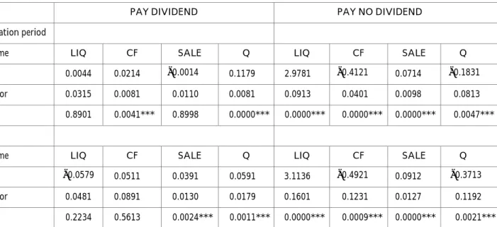
4.1.2. Full period comparison (1992 ~ 1998)
The result from Table 2 (A) reveals that for both groups of firms, investment decisions are under the influence of CF. From Table 2 (B), we know that Q value still has great explanatory power both in Group 1 and Group 2, although there are significant differences of the results between the two groups. This implies that Tobin’s q can indeed reflect a firm’s investment opportunity, especially the confidence interval of Group 2, which is higher than 99 percent. SALE, LIQ and Q have strong explanatory power in both Group 1 and Group 2. Furthermore, CF has totally insignificant results in Group 1, but very significant results in Group 2. This shows that investment in Group 1 is not affected by internal assets but investment in Group 2 is found to be severely affected. This result is identical to the FHP (1988) results. According to the explanation of FHP (1988), under the asymmetric information, companies that face a higher degree of financing constraints are more likely to retain more earnings for investment purposes, due to the high cost of external financing; hence resulting in greater influence on investment decisions. On the other hand, for firms that face less financing constraints, the external financing is less costly. Paying dividends that cause retaining less cash would, therefore, have no negative influence on firms’ investment spending.
4.1.3. Fundamental comparison of the sample groups
From Table 2 it is very clear that when comparing firms based on different types of dividend policy, the extent of investment being influenced by internal assets differs a lot. In other words, firms that pay dividends every year have less financial constraints; on the other hand, firms that pay no dividends every year have greater financial constraints. We can not only predict such differences from firms’ dividend policies, but also from the fundamental information. Comparison results of fundamental discrepancies are presented in Table 3. It reveals that there are great differences in the fundamental comparisons between the two groups of sampling firms, in terms of Growth Rate, Size or ROA. As for Growth Rate, Group 1 is 8.3 percent, on the other hand, Group 2 is 17.1 percent, which is significantly greater than Group 1. But in terms of Size and ROA, Group 1 has significantly greater measure than Group 2. This implies firms in Group 1 are generally bigger in size but have a relatively slow growth rate. Under such circumstances, firms are not bound to retain a great amount of earnings, therefore would choose to pay out cash dividends. However, firms in Group 2 have a greater and faster growing rate, hence are bound to retain more earnings for possible expansion purposes.
•
Chau-Chen Yang, Chung-Jiun Lin & Yi-Chen Lu
PAY DIVIDEND PAY NO DIVIDEND
(A) The whole observation period
Variable Name LIQ CF SALE Q LIQ CF SALE Q
Coefficient 0.0044 0.0214 −0.0014 0.1179 2.9781 −0.4121 0.0714 −0.1831
Standard Error 0.0315 0.0081 0.0110 0.0081 0.0913 0.0401 0.0098 0.0813
Probability 0.8901 0.0041*** 0.8998 0.0000*** 0.0000*** 0.0000*** 0.0000*** 0.0047***
(B) For every year
Variable Name LIQ CF SALE Q LIQ CF SALE Q
Coefficient −0.0579 0.0511 0.0391 0.0591 3.1136 −0.4921 0.0912 −0.3713
Standard Error 0.0481 0.0891 0.0130 0.0179 0.1601 0.1231 0.0127 0.1192
Probability 0.2234 0.5613 0.0024*** 0.0011*** 0.0000*** 0.0009*** 0.0000*** 0.0021***
Note 1: *, ** and *** represents significant at alpha = 0.01, 0.05 and 0.1 level respectively.
Note 2: dependent variable is firm’s gross investment, LIQ = cash on hand at the initial period, CF = gross cash flow of current period, SALE = net sales revenue of last period. Above all three variables are subtracted from the initial total capital stock. Q = Tobin’s q = market value of capital stock/replacement cost of capital stock.
(A) ROA Co mp ariso n Ye ar 199 2 199 3 199 4 199 5 199 6 199 7 199 8 199 2 ~ 19 98 Av erage 1 0 .0 9 7 7 0 .0 8 3 5 0 .0 7 7 1 0 .0 8 7 6 0 .0 7 5 5 0 .0 8 1 7 0 .0 7 9 1 0 .0 8 8 1 Av erage 2 0 .0 2 9 1 0 .0 1 4 0 0 .0 1 7 5 0 .0 4 1 0 0 .0 1 3 0 0 .0 2 3 0 0 .0 1 1 1 0 .0 2 4 3 Proba bility 0 .0 00 0* ** 0.0 0 0 0 * * * 0 .0 00 0* ** 0.0 0 0 0 * * * 0 .0 00 0* ** 0.0 0 0 0 * * * 0 .0 00 0* ** 0.0 0 0 0 * * * (B) S ize Co mp aris o n Ye ar 199 2 199 3 199 4 199 5 199 6 199 7 199 8 199 2 ~ 19 98 Av erage 1 2 1 6 7 7 5 5 8 7 2 2 7 2 5 8 1 8 2 5 4 8 1 9 1 7 2 9 0 6 9 6 7 0 3 2 2 6 2 5 2 5 3 6 1 3 4 1 9 3 2 3 8 3 6 7 8 1 1 8 2 5 2 7 1 4 9 9 Av erage 2 5 5 8 3 8 3 6 6 3 1 6 7 7 1 7 3 9 5 6 2 2 8 9 6 6 6 9 9 1 0 1 4 4 4 6 4 1 0 9 7 1 3 4 1 1 1 3 7 6 2 4 3 6 9 8 9 6 3 1 Proba bility 0 .0 22 5* * 0 .0 18 6* * 0 .0 13 1* * 0 .0 15 7* * 0 .0 16 3* * 0 .0 14 7* * 0 .0 21 1* * 0 .0 00 0* ** Table 3. OLS-Fundamental Comparison
Note 1: *, ** and *** represents significant at alpha = 0.01, 0.05 and 0.1 level respectively. Note 2: Average 1
=
sample average of Group 1; Average 2
=
sample average of Group 2;
T
test = examines whether averages of the two groups are significantly
different; Growth rate
= (Sale t − Sale t − 1)/Sale t =
Revenue Growth Rate * Size
=
Total Assets; ROA
=
NI/TA
=
Return on Assets.
Note 3: The average comparison of growth rate for Average 1 is 8.3146%; Average 2 is 17.1121%;
P (| T |> = t) is 0.16781263, significant at alpha = 0.05.
4.2. Probit Selection Model (PSM)
When proceeding to the second stage analysis, to avoid a bias result, it is essential to make sure that the test of goodness of fit in the first stage is significant. In this paper, all tests of goodness of fit in the first stage models are shown to be significant. Table 4 presents the empirical results and analysis for each research year.
4.2.1. Yearly results of PSM analysis
Year 1992 results are shown in Table 4 (A-1) through (A-3). From Table (A-1), GROW and PR are shown to be two excellent forecasting variables for “pay or not to pay dividend”. Table (A-2) and (A-3) reveals that there is great discrepancy between PAY DIVIDEND and PAY NO DIVIDEND results. Moreover, CF is observed to be significant in Z = 0, implying that investment decisions of firms that pay dividends are not affected by internal capital stock fluctuation; but as for firms that pay no dividends, their investment decisions are under greater influence of internal capital fluctuation. It coincides with FHP (1988). Year 1993 results are shown in Table 4 (B-1) through (B-3). From Table (B-1), it is shown that GROW is a good forecasting variables for “pay or not to pay dividend”. Table 4 (B-2) and (B-3) shows that CF exerts significant influence both on Group 1 and Group 2. In other words, whether firm pays dividends or not, investment decisions are under the influence of internal capital fluctuation. This differs from that concluded in FHP (1988). Year 1994 results are shown in Table 4 (C-1) through (C-3). From Table (C-1), it is shown that PR is a good forecasting variable for “pay or not to pay dividend”. Table 4 (C-2) and (C-3) reveal that there are not many differences between Z = 1 and Z = 0 results. This implies that for both types of firms, the extent to which investment decisions are being affected by internal capital stock fluctuations do not differ a lot. This is different from the conclusion proposed in FHP (1988).
Year 1995 results are shown in Table 4 (D-1) through (D-3). As we can see from Table (D-1), PR and GROWTH are the two good forecasting variables for “pay or not to pay dividend”. In Table 4 (D-2) and (D-3), CF appears to have no influence on both Z = 1 and Z = 0; moreover, results of Z = 1 and
Z = 0 are very similar. This implies that for both types of firms, the extent
to which investment decisions are being affected by internal capital stock fluctuations do not differ a lot. This is different from the conclusion proposed in FHP (1988). Year 1996 results are shown in Table 4 (E-1) ~ (E-3). As we can see from Table (E-1), all of the three variables are good forecasting variables for “pay or not to pay dividend”; GROW is especially significant for p < 0.001.
253
Table
4.
Probit Selection Model
199 2 199 3 (A-1 ) F irst S tage P rob it M o d el (B-1 ) F irst S tage P rob it M o d el Va ria b le N am e Coe ffic ie nt Sta n da rd Error P roba bility V ar ia ble N am e Coe ffic ie nt Sta n da rd Error P roba NI 0 .81 73 1 .23 07 0 .50 66 NI 4 .83 15 1 .54 88 0 .00 18 P R 0 .62 15 0 .29 46 0 .03 49 ** P R 0 .34 13 0 .23 42 0 .14 51 GROW − 0 .58 22 0 .34 21 0 .08 87 * G R O W − 2 .36 09 0 .56 99 0 .00 00 (A-2 ) Z = 1 (p ay d iv id en d ) S eco n d S tage P rob it Mo d el (B-2 ) Z = 1 (p ay d iv id en d ) S eco n d S tage P rob it Mo LI Q 0 .0 14 7 0 .0 87 7 0 .8 66 4 L IQ 0.1 2 9 8 0.0 7 3 9 0.0 7 8 CF 0 .12 14 0 .13 04 0 .35 19 CF − 0 .06 34 0 .02 80 0 .02 38 SA LE − 0 .01 92 0 .02 21 0 .38 60 S A L E 0 .01 77 0 .00 72 0 .01 35 Q 0 .0 20 5 0 .0 49 0 0 .6 75 4 Q 0.0 6 3 6 0.0 3 7 4 0.0 8 8 L A M B DA 0 .20 72 0 .11 86 0 .08 06 * L AM B D A 0 .0 6 1 1 0 .0 6 8 2 0 .3 7 0 (A-3 ) Z = 0 (p ay no d iv id en d ) S eco n d S tage P rob it Mo d el (B-3 ) Z = 0 (p ay no d iv id en d ) S eco n d S tage P S M LIQ − 0 .12 77 0 .12 76 0 .31 72 L IQ − 0 .02 73 0 .02 67 0 .30 69 CF − 0 .77 06 0.0 5 9 8 0.0 0 0 0 * * * C F 0 .0 78 6 0 .0 33 3 0 .0 18 S A L E 0 .18 68 0 .00 33 0 .00 00 ** * S AL E − 0 .00 05 0 .00 15 0 .75 13 Q − 0 .10 33 0.0 8 8 3 0.2 4 2 0 Q 0 .0 19 6 0 .0 44 6 0 .6 60 LA MBD A − 0 .13 97 0 .17 35 0 .42 05 L A M B DA − 0 .18 41 0 .07 60 0 .01 54
254 199 4 199 5 (C-1 ) F irst S tage P rob it M o d el (D-1 ) F irst S tage P rob it M o d el Va ria b le N am e Coe ffic ie nt Sta n da rd Error P roba bility V ar ia ble N am e Coe ffic ie nt Sta n da rd Error P roba NI − 0 .15 66 1 .71 44 0 .92 72 NI − 1 .38 50 1 .31 73 0 .29 31 P R 0 .65 33 0 .26 33 0 .01 30 ** P R 0 .95 42 0 .31 70 0 .00 26 GROW − 0 .04 32 0 .46 93 0 .92 67 GR OW − 0 .76 82 0 .43 60 0 .07 80 (C-2 ) Z = 1 (p ay d iv id en d ) S eco n d S tage P rob it Mo d el (D-2 ) Z = 1 (p ay d iv id en d ) S eco n d S tage P rob it Mo LIQ − 0 .11 74 0 .06 86 0 .08 68 * L IQ 0 .04 50 0 .10 07 0 .65 46 CF 0 .38 57 0 .13 99 0 .00 58 ** * C F 0 .0 9 5 5 0 .1 8 2 5 0 .6 0 0 S A L E 0 .00 64 0 .01 04 0 .53 79 S A L E − 0 .00 53 0 .00 78 0 .49 70 Q 0 .0 16 3 0 .0 47 5 0 .7 32 0 Q − 0 .00 04 0 .03 97 0 .99 11 L A M B DA 0 .09 36 0 .17 86 0 .60 02 L A M B DA 0 .26 42 0 .10 41 0 .01 11 (C-3 ) Z = 0 (p ay no d iv id en d ) S eco n d S tage P rob it Mo d el (D-3 ) Z = 0 (p ay no d iv id en d ) S eco n d S tage P rob it Mo LI Q 4 .6 49 9 0 .0 77 8 0 .0 00 0* ** LI Q 0 .0 15 2 0 .0 80 6 0 .8 50 CF − 0 .67 39 0 .11 73 0 .00 00 ** * C F 0 .0 6 1 4 0 .0 6 5 9 0 .3 5 1 S A L E 0 .04 78 0 .04 00 0 .23 15 S A L E 0 .00 21 0 .00 76 0 .77 87 Q 0 .0 58 0 0 .2 56 5 0 .8 21 1 Q 0.0 2 9 7 0.0 4 2 6 0.4 8 4 L A M B DA 0 .96 35 0 .54 16 0 .07 52 * L AM B D A − 0 .15 64 0 .10 70 0 .14 39 Table 4 . (Continued)
255 199 6 199 7 (E -1 ) F irst S tage P rob it M o d el (F -1 ) F irst S tage P rob it M o d el Va ria b le N am e Coe ffic ie nt Sta n da rd Error P roba bility V ar ia ble N am e Coe ffic ie nt Sta n da rd Error P roba NI 6 .81 08 1 .76 70 0 .00 01 ** * N I − 0 .16 96 1 .74 12 0 .41 32 PR 0.5 0 4 9 0.2 8 3 1 0.0 7 4 4 * P R 0 .7 73 1 0 .2 69 2 0 .0 04 GROW − 2 .00 60 0 .45 07 0 .00 00 ** * G R O W − 0 .08 11 0 .53 19 1 .21 03 (E-2 ) Z = 1 (p ay d iv id en d ) S eco n d S tage P rob it Mo d el (F -2 ) Z = 1 (p ay d iv id en d ) S eco n d S tage P rob it Mo LIQ − 0 .13 29 0 .09 99 0 .18 36 L IQ − 0 .14 31 0 .07 78 0 .07 12 CF 0 .07 75 0 .07 18 0 .28 04 CF 0 .31 47 0 .11 31 0 .00 50 S A L E 0 .00 55 0 .00 69 0 .42 75 S A L E 0 .00 51 0 .00 91 0 .51 61 Q 0 .1 15 9 0 .0 37 0 0 .0 01 7* ** Q 0 .0 17 6 0 .0 31 2 0 .5 00 LA MBD A − 0 .01 91 0 .08 32 0 .81 88 L A M B DA 0 .19 01 0 .10 12 0 .05 12 (E-3 ) Z = 0 (p ay no d iv id en d ) S eco n d S tage P rob it Mo d el (F -3 ) Z = 0 (p ay no d iv id en d ) S eco n d S tage P rob it Mo LIQ − 0 .31 76 0.3 0 1 7 0.2 9 2 5 LI Q 2 .1 24 2 0 .0 93 2 0 .0 00 CF 1 .00 89 0 .08 99 0 .00 00 ** * C F − 0 .76 19 0 .12 91 0 .00 00 S A L E 0 .00 70 0 .02 77 0 .80 15 S A L E 0 .09 16 0 .06 89 0 .17 13 Q 0 .0 94 2 0 .2 03 6 0 .6 43 6 Q 0.0 4 9 2 0.2 1 3 3 0.9 1 0 LA MBD A − 0 .00 78 0 .36 83 0 .98 32 L A M B DA 0 .51 51 0 .21 07 0 .01 91 Table 4 . (Continued)
256 199 8 199 2 ~ 19 98 (G-1 ) F irst S tage Pro b it Mo de l (H-1 ) F irst S tage Pro b it Mo de l Vari ab le Name Coe ffic ie nt Stand ard Erro r Proba bility Vari ab le Name Coe ffic ie nt Stand ard Erro r Proba bility NI − 1 .13 01 1 .12 31 0 .30 12 NI 1 .41 61 0 .74 50 0 .05 91 PR 0 .82 41 0 .24 96 0 .01 12 ** * PR 0 .50 11 0 .26 15 0 .04 12 GROW − 0 .61 42 0 .47 20 0 .19 78 GROW 0 .98 15 0 .21 32 0 .00 00 (G-2 ) Z = 1 (p ay d iv id en d ) S eco n d S tage Pr o b it M ode l (H-2 ) Z = 1 (p ay d iv id en d ) S eco n d S tage Pr o b it M ode LIQ 0 .05 43 0 .11 61 0 .61 12 LIQ 0 .00 14 0 .02 11 0 .99 92 CF 0 .08 74 0 .17 31 0 .50 13 CF 0 .01 31 0 .00 60 0 .02 97 SA LE − 0 .00 62 0 .00 82 0 .49 99 SA LE 0 .00 05 0 .00 10 0 .59 21 Q − 0 .01 10 0 .04 12 0 .77 21 Q 0 .02 17 0 .01 89 0 .20 18 LA MBD A 0 .21 47 0 .09 13 0 .02 01 ** LA MBD A 0 .24 13 0 .04 98 0 .00 00 (G-3 ) Z = 0 (p ay no d iv id en d ) S eco n d S tage Pr o b it M ode l (H-3 ) Z = 0 (p ay no d iv id en d ) S eco n d S tage Pr o b it M LIQ 0 .01 79 0 .08 46 0 .79 98 LIQ 3 .01 12 0 .09 13 0 .00 00 CF 0 .07 31 0 .07 05 0 .31 22 CF − 0 .54 71 0 .03 13 0 .00 00 SA LE 0 .00 42 0 .01 41 0 .69 00 SA LE 0 .07 93 0 .00 73 0 .00 00 Q 0 .02 73 0 .03 71 0 .51 04 Q 0 .05 17 0 .17 21 0 .69 28 LA MBD A − 0 .14 97 0 .09 12 0 .09 12 * LA MBD A 0 .91 20 0 .30 12 0 .00 17 Table 4 . (Continued)
Note 1: *, ** and *** represents significant at alpha
=
0.01, 0.05 and 0.1 level respectively.
Note 2: regression variable
=
whether firms pay dividends, NI
=
gross income after tax, PR
=
cash dividend of previous financial peri
od, GROW
=
Revenue Growth Rate
t − Sale t − 1)/Sale t. Note 3: Z = 0
represents “pay no dividends”;
Z
=
1
represents “pay dividends”.
Note 4: regression variable
=
firm’s gross investment; LIQ
=
cash on hand at the initial period; CF
=
gross cash flow of current peri
od; SALE
=
net sales revenue of last
period. Above three variables are all subtracted from the initial total capital stock. Q
=
Tobin’s
q
=
Table (E-2) and (E-3) reveal that there are great differences between Z = 1 and Z = 0 results in which CF and Q show significant influence for Z = 0. In other words, investment decisions of firms that pay no dividend are under greater influence from internal capital fluctuations; as for firms with dividend policies, investment decisions are under less influence from internal capital fluctuations. This coincides with the conclusions proposed in FHP (1988). Year 1997 results are shown in Table 4 (F-1) through (F-3). As we can see from Table 4 (F-1), PR is a good forecasting variable for “pay or not to pay dividend”. Table 4 (F-2) and (F-3) reveal that there are not many differences between Z = 1 and
Z = 0 results. This implies that for both types of firms, the extent to which
investment decisions are being affected by internal capital stock fluctuations do not differ a lot. This is different from the conclusion proposed in FHP (1988). Year 1998 results are shown in Table 4 (G-1) through (G-3). As we can see from Table (G-1), PR is a good forecasting variable for “pay or not to pay dividend”. Table (G-2) and (G-3) reveal that there are not many differences between Z = 1 and Z = 0 results. This implies that for both types of firms, the extent to which investment decisions are being affected by internal capital stock fluctuations do not differ a lot. This is different from the conclusion proposed in FHP (1988).
4.2.2. Full Period Comparison (1992 ~ 1998)
The full period comparison results are shown in Table 4 (H-1) through (H-3). It is shown in Table (H-1) that all of the three variables appear to be good forecasting variables for “pay or not to pay dividend”; in particular, PR and GROW are significant for p < 0.001. Table (H-2) and (H-3) reveal that the differences between Z = 1 and Z = 0 results are not significant, in which CF has influence on both Z = 1 and Z = 0. This also implies the extent of the investment decisions being affected by internal capital stock fluctuations is indifferent, which deviates from the conclusion proposed in FHP (1988). Results of previous subsections are compared and presented in the following charts:
Chart 1– Chart 4 show the differences between OLS model and Probit Selection model PSM (two stage transitional model) by comparing the empirical results of each variable derived from the two models. As to the extent of how LIQ influences investment, comparison results in Chart 1 reveal that OLS and PSM results are almost indifferent except for year 1994, 1996 and 1997. As to the extent of how SALE influences investment, Chart 2 shows that in year 1993 and 1997, it is significantly different by applying OLS and PSM model. Chart 3 shows the extent of how Tobin’s q influences investment, results derived
Comparison of the two methods — LIQ CHART 1
Two Stage Model OLS Model
GroupYear Z = 1 Pay Dividends Z = 0 Pay no Dividends Z = 1 Pay Dividends Z = 0 Pay no Dividends 1992 1993 + + 1994 + + + 1995 1996 + 1997 + + 1998 1992 ~ 1998 Sample A + + 1992 ~ 1998 Sample B +
Note 1: + represents significance at the 0.05 significance level (one-tail).
Note 2: sample A includes firms that pay cash dividends every year, and sample B pay no cash dividends at all for the whole period under study.
Comparison of the two methods — SALE CHART 2
Two Stage Model OLS Model
GroupYear Z = 1 Pay Dividends Z = 0 Pay no Dividends Z = 1 Pay Dividends Z = 0 Pay no Dividends 1992 + 1993 + + 1994 1995 1996 1997 + 1998 1992 ~ 1998 Sample A + + 1992 ~ 1998 Sample B + +
Note 1: + represents significance at the 0.05 significance level (one-tail).
Note 2: sample A includes firms that pay cash dividends every year, and sample B pay no cash dividends at all for the whole period under study.
Comparison of the two methods — Q CHART 3
Two Stage Model OLS Model
GroupYear Z = 1 Pay Dividends Z = 0 Pay no Dividends Z = 1 Pay Dividends Z = 0 Pay no Dividends 1992 + 1993 + + + 1994 + 1995 + + 1996 + + 1997 1998 + + 1992 ~ 1998 Sample A + + 1992 ~ 1998 Sample B + +
Note 1: + represents significance at the 0.05 significance level (one-tail).
Note 2: sample A includes firms that pay cash dividends every year, and sample B pay no cash dividends at all for the whole period under study.
Comparison of the two methods — CF CHART 4
Two Stage Model OLS Model
GroupYear Z = 1 Pay Dividends Z = 0 Pay no Dividends Z = 1 Pay Dividends Z = 0 Pay no Dividends 1992 + + 1993 + + + + 1994 + + + + 1995 1996 + + 1997 + + 1998 + 1992 ~ 1998 Sample A + + + + 1992 ~ 1998 Sample B +
Note 1: + represents significance at the 0.05 significance level (one-tail).
Note 2: sample A includes firms that pay cash dividends every year, and sample B pay no cash dividends at all for the whole period under study.
from OLS model and PSM appear to be significantly different for almost all research years and full period comparison except for year 1996, 1997 and 1998. Moreover, it is worth to mention that Tobin’s q in OLS model is an excellent explanatory variable as it is shown to be significant in most research years. However, the reverse is observed in Z = 0 category of PSM as Tobin’s q appears to be insignificant for all research years. Therefore OLS and PSM results are concluded to be significantly different from each other.
As to the extent of how CF influences investment, comparison results in Chart 4 reveal that OLS and PSM have similar results of how internal capital fluctuation affects investment in year 1992 to 1996. Particularly, year 1992 and 1996 are significant in terms of different dividend policies; that is, as for
Z = 1, results show that investment is not influenced by cash flow and vice
versa for Z = 0. This coincides with previously stated theory, i.e. when firms face more financing constraints, more internal capital will be retained for investment purpose, therefore it will forego paying cash dividend, which implies that investment is bound to internal capital fluctuations. As for year 1993 and 1994, no significant differences can be observed as all results reveal that cash flow do have great influence on investment. This implies that all firms are facing financing constraints to various extents no matter they are paying dividends or not. However, as for year 1995 result, all results reveal that investments are not under the influence of cash flow, in other words, whether firms pay dividend or not, their investments do not have financing constraints.
The whole period (1992 ~ 1998) comparison for OLS shows that for firms that pay dividends every year, their investment are under less influence of internal capital stock. On the other hand, for firms that do not pay dividends every year, their investments are under influence of internal capital stock. It is just what the theory implies: firms that are not facing financial constraints are able to access external capital more easily; even though the cash dividend policy will decrease internal capital stock, their investments will not be subjected to a great fluctuation. Besides, we can also see from Table 3, the size of the firms that pay dividends every year is not as big as that of the firms that do not pay dividends every year. However, firms that do not pay dividends every year have smaller growth rate than that of firms with annual dividend policy. These two observations give the justification for what the theory states: big firms have less financial constraints than small firms, moreover, firms that generally have higher growth rates are those belonging to younger industries. In terms of maturity of industry, it implies that firms belonging to mature industries experience less financing constraints than that of young industries.
5. Conclusions
If the capital market is imperfect, asymmetric information and the agency problem will cause a firm to face financing constraints. When a firm has financing constraints, meaning that the firm can not access external financing easily, it may have to retain more earnings in order to supply its investment needs. If a firm has a good investment opportunity, but has to give it up just because the firm cannot have enough capital from financing, the problem of underinvestment arises. The firm whose investment counts more heavily on internal financing has more investment-cash flow sensitivity. Fazzari, Hubbar, and Petersen (1988) propose the initial use of investment-cash flow sensitivity in order to investigate whether the firm has financing constraints. They categorize samples according to dividend pay out rate, then apply Q model, acceleration model and neo-classic model for empirically testing the differences among categories. Later researchers such as Devereux and Schiantarelly (1989), Hoshi, Kashyap and Scharfstein (1991) all followed FHP’s method to conduct more financing constraints related research.
FHP (1988) believe that after controlling the factor that affects investment opportunities (Tobin’s q), if the firm faces greater problems in financing constraints, it will retain more internal capital stock (hence reduce cash dividend pay out). Therefore its investment will be affected by cash flow to a greater extent. However, the sample categorizing method of FHP has received much controversy. For example, Schaller (1993) points out that the sample categorizing standard is of an “endogenous” nature and, therefore, is not suitable to use in a regression model. Whited (1992), on the other hand, points out that investment and dividend policy are simultaneously used to make decisions within a firm, therefore it is not appropriate to directly use dividend pay out rate as the sample categorizing method. More criticisms also come from Kaplan and Zingales (1997). This paper applies a methodology that differs from other scholars’ in that samples are separated into some groups according to certain criteria, and the differences of investment–cash flow sensitivity among groups are examined in order to find out whether there exists any financing constraint difference. The probit Selection Model is used for categorizing the sample according to their retention ratios, and Q model applies next in order to examine the difference of financing constraints. The research sets off from investment theory, uses more robust methodology, and discusses information asymmetry and agency problem by examining the financing constraints of the firm.
5.1. Investment function and cash flow
(1) Short run
From this paper’s empirical result we can see that using the OLS or Probit Selection model, the extent of how investment is being affected by cash flow for the two categorized sampling groups differs insignificantly. During the research period, only year 1992 and 1996 results show significant differences, which implies that investment of firms that pay dividends has been significantly affected by cash flow; and vice versa for firms that do not pay dividends. However, for year 1993 and 1994 results which are compared to be indifferent, investment of each sampling firm has been affected significantly by cash flow. To sum up from the results of each research period, sampling firms that “pay no dividends” has been affected greatly by internal capital stock, which implies a situation of facing severe financing constraints. However, it is not implied for sampling firms that ”pay dividends”. Therefore, based on empirical results of each research period, “pay dividends or not” can not be used as sampling categorization in the regression model in order to judge whether there are significant differences among firms.
(2) Long run
When we extend the research period from year 1992 to 1998, then the OLS empirical results show that there exist significant differences between the two sampling firms. As for firms that did not pay dividends every year during the research period, investment appears to be influenced by cash flow. This implies that if the firm pays a cash dividend annually, then the problem of financing constraints is less likely to happen. In other words, the firm’s investment is not under the influence of internal capital stock; furthermore, investment decisions are not closely related to the dividend policy. If the firm does not pay any cash dividend in order to retain the majority of earnings, it implies that it faces more financial constraints. In other words, investment of the firm will be affected greatly by its internal capital stock. To sum up, in order to achieve a more accurate answer about whether firms face financing constraints, the period of research should cover a longer horizon.
5.2. OLS model and Probit Selection Model
This paper not only applies the traditional OLS model, but also another transitional model, namely the Probit Selection Model that considers the hypothesized relationship between the investment decisions and dividend policy
within a firm. The empirical results of the two models are not the same such that the greatest discrepancy took place in the influence of Q value. In the OLS model, Q (Tobin’s q) is an excellent explanatory variable; however, in the Probit Selection Model, it is not. This implies that if using the Probit Selection Model to separate sampling firms into groups is a must. However if instead we apply the OLS model to separate sampling firms into groups directly, then significant bias will appear. In this paper, these two types of models produced almost indifferent empirical results for answering whether the two groups of sampling firms are facing financing constraints. In other words, in the research period, only the years 1992 and 1996 did the results show that there is a different extent of financing constraints for firms that pay dividends or not.
5.3. Nonexistence of perfect capital market
Under an imperfect capital market, since there are various factors affecting firms to finance through external sources, therefore, firms are said to have financing constraints. This paper provides another empirical testing method in order to examine whether the capital market is perfect or not. Due to the fact that the firms’ investment is under the influence of internal capital fluctuation, which further implies that there exists no company that can access external financing smoothly in order to fund the required capital. To sum up, this paper would like to propose that the cause of imperfect capital markets might be due to the presence of asymmetric information and agency problems.
References
Blose, Laurence E. and Joseph C.P. Shieh, 1997, “Tobin’s q-ratio and market reaction to capital investment announcements”, The Financial Review Vol. 32 No. 3, 449 – 476.
Brainard, William C. and James Tobin, 1968, “Pitfalls in financial model building”, American Economic Review 58, 99– 122.
Calem, Paul S. and John A. Rizzo, 1995, “Financing constraints and investment: New evidence from hospital industry data”, Journal of Money, Credit and Banking 27, No. 4, 1002– 1014.
Chirinko, Robert S., Huntley Schaller, 1995, Journal of Money, Credit and Banking 27, 527– 548.
Devereux, Michael, Fabio Schiantarelli, 1989, “Investment, financial factors and cash flow: Evidence from UK panel data”, NBER working paper No. 3116.
Faroque, Akheter and T. Ton-That, 1995, “Financing constraints and firm heterogeneity in investment behavior: An application of non-nested tests”, Applied Economics 27, 317– 326.
Fazzari, Steven M., R. Glen Hubbard, Bruce C. Petersen, 1996, “Asymmetric information, financing constraints and investment”, Review of Economics and Statistics 69, 481– 488.
Fazzari, Steven M, R. Glenn Hubbard, Bruce C. Petersen, 1996, “Financing constraints and corporate investment: Response to Kaplan and Zingales”, NBER working paper No. 5462.
Fazzari, Steven M., R. Gleen Hubard, Bruce C. Petersen, 1988, “Financing constraints”, Brookings Papers on Economic Activity, pp. 141– 206.
Galeotti, Marzio, Fabio Schiantarelli and Fidel Jaramillo, 1994, “Investment decisions and the role of debt, liquid assets and cash flow: Evidence from Italian panel data”, Applied Financial Economics 4, 121– 132.
Gilchrist, Simon, Charles P. Himmelberg, 1995, “Evidence on the role of cash flow for investment”, Journal of Monerary Economics 36, 541– 572.
Green, W. H. 1992, “Limdep-user’s manual and reference guide”, New York: Econometric Software, Inc.
Hayshi Fumio, 1982, “Tobin’s marginal q and average q: A neoclassical interpretation”, Econometrica 50, 213– 224.
Hoshi, Takeo, Anil Kashyap, David Scharfstein, 1991, “Corporate structure, liquiity and investment: Evidence from Japanese industrial groups”, Quarterly Journal of Economics 106, 33– 60.
Jahera, John, William Lloyd, and Naval Modani, 1986, “Growth, beta and agency costs as determinants of dividend”, Akron Business and Economic Review 17, 55– 69. Jose, Manual L., Len M. Nichols and Jerry L. Stevens, 1986, “Contributions of
diversification promotion and R&D tot he value of multiproduct firms: A Tobin’s q approach”, Financial Management 15, 33– 42.
Kaplan, Steven N. and Luigi Zingales, 1995, “Do financing constraints explain why investment is correlated with cash flow?”, Working Paper No. 5267, National Bureau of Economic Research.
Kaplan, Stenev N. and Luigi Zingales, 1997, “Do investment-cash flow sensitivities provide useful measures of financing constraints?”, Quarterly Journal of Economics 1, 169– 215.
Lamont, Owen, 1997, “Cash flow and investment: Evidence from internal capital markets”, Journal of Finance LII, 83– 109.
Lang, Larry, Eli Ofek and Rene M. Stulz, 1996, “Leverage, investment and firm growth”, Journal of Financial Economics 40, 3– 29.
Lee, Bong-Soo, Tom Nohel, 1997, “Value maximization and the information content of corporate investment with respect to earnings”, Journal of Banking and Financing 21, 661– 683.
Lewellen, Wibur G., S. G. Badrinah, 1997, “On the measurement of Tobin’s q”, Journal of Financial Economics 44, 77– 122.
Lindenberg, Eric B. and Stephen A. Ross, “Tobin’s q ratio and industrial organization”, Journal of Business 54, 1– 32.
Lintner J., 1956, “Distribution of incomes of corporations among dividends retained earnings and taxed”, American Economic Review.
Miller, Merton and Franco Modigliani, 1961, “Dividend policy, growth and the valuation of shares”, Journal of Business.
Modigliani, Franco and Merton Miller, 1958, “The cost of capital, corporation finance and the theory of investment”, American Economic Review 8, 261– 297.
Myers, Stewart C. and Nicholas S. Majluf, 1984, “Corporate Financing decisions when firms have investment information the investors do not”, Journal of Financial Economics 13, 187– 221.
Partington, Garaham H., 1987, “Variables influencing dividend policy in Australia: Survey results”, Journal of Business Finance and Accounting 16, 165– 182.
Ramirez, Carlos D., 1995, “Did J. P. Morgan’s men add liquidit? Corporate investment, cash flow ad financial structure at the turn o the twentieth century”, Journal of Finance L, 661– 678.
Roseff, Michael S., 1982, “Growth, beta, and agency cost as determinants of dividend payout ratios”, Journal of Financial Research 5, 249– 259.
Schaller, Huntley, 1993, “Asymmetric information, liquidity constraints and Canadian investment”, Canadian Journal of Economics 26, 552– 574.
Stiglitz, Joseph and Andrew Weiss, 1981, “Credit rationing in markets with imperfect information”, American Economic Review 71, 393– 401.
Tinbergen, Jan., 1939, “A method and its application to investment activity”, in Statistical Testing of Business Cycle Theories Vol. 1.
Tobin, James, 1969, “A general equilibrium approach to monetary theory”, Journal of Money, Credit and Banking 1, 15– 29.
Whited, Toni M. 1992, “Debt, liquidity constraints and corporate investment: Evidence from panel data”, Journal of Finance XL, 1425– 1460.