條件風險值限制下之最適保險契約

行政院國家科學委員會專題研究計畫 成果報告

條件風險值限制下之最適保險契約

研究成果報告(精簡版)

計 畫 類 別 ： 個別型 計 畫 編 號 ： NSC 100-2410-H-151-013- 執 行 期 間 ： 100 年 08 月 01 日至 101 年 07 月 31 日 執 行 單 位 ： 國立高雄應用科技大學財經與商務決策研究所 計 畫 主 持 人 ： 汪青萍 共 同 主 持 人 ： 黃鴻禧 計畫參與人員： 碩士班研究生-兼任助理人員：李香怡 碩士班研究生-兼任助理人員：李秀錡 公 開 資 訊 ： 本計畫可公開查詢

中 華 民 國 101 年 10 月 23 日

中 文 摘 要 ： 本研究分別導出在被保險人或保險人受條件風險值限制下之 最適保險契約。但在實務上，條件風險值乃根據風險值算 出，故條件風險值之限制經常伴隨著風險值之限制。因此， 本研究所導出的最適保險契約同時加入風險值與條件風險值 的限制。研究結果發現無論是被保險人或保險人受限於風險 值與條件風險值，兩者之最適保險型式皆類似。其次，最適 保險契約可分為兩種類別。其一為不受到風險值與條件風險 值限制的標準自負額保險；另外為雙重自負額保險及其四種 退化型式。 中文關鍵詞： 最適保險契約；雙重自負額保險；風險值；條件風險值 英 文 摘 要 ： This study develops an optimal insurance form under

the insured＇s and insurer＇s CVaR constraints,

respectively. Since CVaR value is based on calculated VaR value, the developed insurance contacts

simultaneously meet the VaR and CVaR constraints. This study finds that the insurance contractual forms with the insured＇s VaR and CVaR constraints are analogous to the insurer＇s ones. Additionally, the possible contractual forms have two categories. The first is a standard deductible insurance where the VaR and CVaR constraints are not binding. The next category contains a double deductible insurance and its four degenerative forms.

英文關鍵詞： Optimal insurance contract； double deductible insurance； VaR； CVaR

Optimal Insurance Contract under CVAR Constraint

Abstract

This study develops an optimal insurance form under the insured’s and insurer’s CVaR constraints, respectively. Since CVaR value is based on calculated VaR value, the developed insurance contacts simultaneously meet the VaR and CVaR constraints. This study finds that the insurance contractual forms with the insured’s VaR and CVaR constraints are analogous to the insurer’s ones. Additionally, the possible contractual forms have two categories. The first is a standard deductible insurance where the VaR and CVaR constraints are not binding. The next category contains a

double deductible insurance and its four degenerative forms.

條件風險值限制下之最適保險契約

摘要

本研究分別導出在被保險人或保險人受條件風險值限制下之最適保險契 約。但在實務上，條件風險值乃根據風險值算出，故條件風險值之限制經常伴隨 著風險值之限制。因此，本研究所導出的最適保險契約同時加入風險值與條件風 險值的限制。研究結果發現無論是被保險人或保險人受限於風險值與條件風險 值，兩者之最適保險型式皆類似。其次，最適保險契約可分為兩種類別。其一為 不受到風險值與條件風險值限制的標準自負額保險；另外為雙重自負額保險及其 四種退化型式。 關鍵字：最適保險契約；雙重自負額保險；風險值；條件風險值。

1. Introduction

This study aims to develop the optimal insurance policy form endogenously under a conditional value-at-risk (CVaR) framework, where CVaR is the expected value of the losses exceeding VaR (value-at-risk).1 No matter the institutions or individuals frequently face different forms of risk, and most of which can be insured. As CVaR is treated as a risk management tool, it is natural for institutions or individuals facing different forms of risk to purchase insurance reducing risk to meet their CVaR criteria. In this study, two topics are discussed. The first concerns on “optimal insurance contract under insured’s CVaR constraint”, in which the insured’s objective is to maximize expected wealth utility, but has a CVaR constraint to be met. Although Wang et al. (2005) and Huang (2006) had examined this similar problem, their risk management criterion is VaR. Different from Wang et al. (2005) and Huang (2006), this study adopts CVaR as risk management tool to explore the optimal insurance policy form.

When an insurer offers an insured an insurance contract, he/she will take on the insured’s risk and thus will be faced with some risk exposure. Indeed, after paying an indemnity to the insured, the insurer may be subject to large losses. Therefore, the second topic addresses “optimal insurance contract under the insurer’s CVaR constraint”, in which the insured maximizes the expected wealth utility subject to the insurer’s CVaR constraints. Related researches regarding the optimal insurance with the insurer’s risk constraint are as follows. Zhou and Wu (2009) developed the optimal insurance under the insurer’s VaR constraint. Zhou and Wu (2008) derived the optimal insurance under the insurer’s risk constraint, where the risk constraint is that

1 _{Value at Risk (VaR) is a risk measure for financial risk management and widely used is in practice.} VaR is defined as the worst expected loss over a given horizon at a given confidence level, such as 95

the expected loss of the insurer’s terminal wealth after the payment is maintained below some prespecified level. Additionally, Zhou et al. (2010) derived the optimal insurance in the presence of insurer’s loss limit, where the loss limit means that the insurer wishes to limit the loss after the payments below some prespecified level. However, in our knowledge, this study is the only work in developing the optimal insurance under insured’s or insurer’s CVaR constraint. Nevertheless, the CVaR value is based on the calculated VaR value. Thus, CVaR constraint frequently accompanies VaR constraint. Consequently, this study will further consider the optimal insurance contract which simultaneously meets VaR and CVaR constraints.

In this study, using CVaR instead of VaR as a risk measure tool is motivated by the following reasons. First, some studies had presented the deficiencies of VaR and also suggested CVaR as a risk measure tool. (Szegö, 2002; Tasche, 2002; Acerbi and Tasche, 2002) Alexander et al. (2006) recognized that VaR has some limitations: lacking subadditivity and convexity. Therefore, the VaR of the combination of two portfolios can be greater than the sum of VaR of the individual portfolios. Moreover, the problem of minimizing a portfolio VaR can have multiple local minimizers. Rockafellar and Uryasev (2002) stated that VaR suffers from being unstable and difficult to work with numerically when losses are not normally distributed. They suggested an alternative measure, CVaR, as a tool in optimization modeling. Moreover, Kibzun and Kuznetsov (2006) noted that if the loss function is convex in a strategy, then CVaR is convex in the strategy. This property is very convenient for optimization. Second, indeed, practitioners and regulators are usually more concerned with the risk exposure in terms of the size of potential losses, since a catastrophic event may completely wipe out an investment. However, VaR mainly depends on the probability of losses but not on their values. Kuan (2009) expressed that an

undesirable property of VaR measure is that it is insensitive to the magnitude of extreme losses. CVaR concerns about the loss magnitude. Accordingly, this paper adopts CVaR as a risk management tool.

Much literature addresses the CVaR topic, which can be roughly divided into two categories. The first category primarily focuses on the CVaR calculation and estimation. For instance, Rockafellar and Uryasev (2002) furnished an elementary way of calculating CVaR directly. Additionally, Sun and Hong (2010) estimated CVaR by using importance-sampling techniques; they derived the asymptotic estimator of CVaR and proved its consistency and asymptotic normality. The second category mainly employed CVaR to portfolio optimization problem. Andersson et al. (2001) analyzed a portfolio of bonds issued in emerging markets and minimized the credit risk using the minimum CVaR approach. Next, Topaloglou et al. (2002) developed a CVaR model for optimal selection of international portfolios incorporating currency hedging decisions within the portfolio selection model. Moreover, Alexander et al. (2006) analyzed the problem of computing the optimal CVaR portfolios, with the addition of a proportional cost. Alexander et al. (2007) examined the impact of adding a CVaR constraint to the mean–variance model assuming that returns have a discrete distribution with finitely many jump points. Furthermore, Quaranta and Zaffaroni (2008) dealt with a portfolio selection model by applying the methodology of robust optimization to minimize the CVaR of a portfolio. As above mentioned, CVaR has been an acceptable risk measure tool and has been applied to many situations.

Various investigations have examined optimal insurance contract forms. For example, Raviv (1979) showed that the optimal insurance form is full insurance above a straight deductible or coinsurance above the deductible, given different assumptions.

Subsequent many studies followed and extended Raviv (1979) work. (Doherty and Schlesinger, 1983; Gollier, 1987, 1996; Vercammen, 2001; Ermoliev and Flam, 2001) Additionally, Zhou et al. (2008) discussed the optimal insurance strategy to maximize the expected utility of terminal wealth of risk-averse individual under an intertemporal equilibrium. It is shown that the individual’s optimal insurance strategy actually is equivalent to buying a put option written on his/her holding asset with a proper strike price. Moreover, Zhuang et al. (2009) established orderings of optimal allocations of policy limits and deductibles considering loss severities and loss frequencies by maximizing the expected wealth utility of the policyholder. In our knowledge, no literature addresses the optimal insurance contract under CVaR framework.

The creator of the term value at risk is from J.P. Morgan in the late 1980s. The major inspiring principles of the 2001 proposal of the Basel Banking Supervisory Committee suggested that VaR was assumed as risk measure. (Szegö, 2005) Nowadays, VaR has been a very popular risk measure of downside risk and widely used by financial institutions to watch over their exposures and regulators to set margin, although the literature noted the drawback of VaR. Basak and Shapiro (2001) stated that the wide usage of the VaR-based risk management by financial as well as nonfinancial firms stems from the fact that VaR is an easily interpretable summary measure of risk and also has an appealing rationale, as it allows its users to focus attention on “normal market conditions” in their routine operations. Indeed, VaR measures downside risk and is a compact representation of risk level. (Szegö, 2002) Therefore, Wang et al. (2005) applied VaR to optimal insurance contract. They designed an optimal insurance contract which the objective of the insured is to maximize the expected final wealth under the VaR constraint. Assuming the insurance

loading to be proportional to expected indemnity, the optimal insurance policy form is endogenously derived. The results showed that the optimal insurance policy can be replicated by three options, including a long call option with a small strike price, a short call option with a large strike price, and a short cash-or-nothing call option. Later, Huang (2006) extended Wang et al. (2005) and further considered a more realistic situation where the insured is risk averse instead of the Wang’s assumption that the insured is risk neutral. The objective function is to maximize expected utility rather than expected wealth in Wang et al. Owing to the VaR constraint, the optimal insurance schedule cannot be solved by variations of calculus. Accordingly, Huang proposed a new approach to derive the optimal insurance. The optimal insurance contract under the VaR constraint is a single deductible insurance when the VaR constraint is redundant or a double deductible insurance when the VaR constraint is binding. Furthermore, Cai et al. (2008) used VaR criterion to the reinsurance problem. By formulating a reinsurance optimization problem that minimizes the VaR of an insurer’s total cost, they pointed out that the forms for optimal reinsurance depend on the confidence level for the risk measure and the safety loading for the reinsurance premium.

As above stated, by maximizing the insured’s expected wealth or utility, the optimal insurance is generally developed from the insured’s viewpoint. When faced with the uncertainty of loss, the insured can buy an insurance contract and transfer some risk to the insurer. However, for the insurer, when the insurance policy with no limit on coverage, the insurer can be under a heavy financial burden, especially when the insured suffers a large unexpected loss. Accordingly, imposing the insurer’s risk constraint on the optimal insurance problem is very important. Little attention has been paid on the controlling of the insurer’s risk exposure. Zhou and Wu (2008)

examined the optimal insurance problem under the situation that the insured maximizes the expected utility of his /her terminal wealth, subject to the constraint that the expected loss of the insurer’s terminal wealth is maintained below some exogenously specified level. It is shown that when the insurer’s risk constraint is binding, the optimal insurance is not linear but piecewise linear deductible. Additionally, if the risk tolerance for the insurer is increased, the insured’s optimal expected utility will increase. Additionally, Zhou et al. (2010) considered the optimal insurance problem with a constraint which the insurer limits the loss after the payments below some prespecified level. Coverage above a deductible up to a cap is shown to be optimal when the insurance price depends only on the policy’s actuarial value, and when the insured seeks to maximize the expected utility of his terminal wealth. Relaxation insurer's loss limit will increase the insured's expected utility. Moreover, Zhou and Wu (2009) developed the optimal insurance, in which the insured aims to maximize his expected utility of terminal wealth under the constraint that the insurer wishes to control the VaR of his terminal wealth to be maintained below a prespecified level. It is shown that when the insurer’s VaR constraint is binding, the solution to the problem is not linear, but piecewise linear deductible, and the insured’s optimal expected utility will increase as the insurer becomes more risk-tolerant. In the second project, we will impose the insurer’s risk constraint on the optimal insurance to develop the optimal insurance contract under the CVaR framework.

Referring to Huang (2006), Zhou and Wu (2008), Zhou and Wu (2009) and Zhou et al. (2010), this study assumes the insured is risk averse and the insurance premium is a function of expected indemnity. This study aims to discuss the optimal insurance form in which the insured or the insurer is imposed by a CVaR constraint.

Accordingly, this study can be divided into two main parts. This first aims to develop the optimal insurance form under the insured’s CVaR constraint while the second focuses on the insurer’s CVaR constraint. In practice, we first calculate the VaR value given a particular confidence level, 1, then the CVaR value is based on the calculated VaR value. Consequently, this study will further consider the optimal insurance contract which simultaneously meets the VaR and CVaR constraints.

The remainder of this study is organized as follows. Section 2 presents the assumptions and definitions for the two projects. The assumptions include the probability distribution of loss, the utility function of the insured, the insurance premium, etc. The definitions mainly include the mathematical presentations for VaR and CVaR. Next, Section 3 reviews the related literature focusing on the optimal insurance contract under VaR or risk constraint. The literature include Wang et al. (2005), Huang (2006), Zhou and Wu (2008), Zhou and Wu (2009) and Zhou et al. (2010). Subsequently, Section 4 develops the optimal insurance form in which the insured or the insurer is imposed by a VaR and CVaR constraint. Finally, Section 5 provides our conclusions and future research directions.

2. Assumptions and Definitions

Referring to Raviv (1979), Gollier (1996), Wang et al. (2005), Huang (2006) and Zhou and Wu (2009), this study makes the following assumptions. An insured has an initial endowment, E₁, and faces a risk of loss, X, which is a non-negative continuous

random variable with probability density function, f(x) and cumulative distribution function, )F(x . An insurer with an endowment, E₂, provides an insurance policy to

reduce this risk. The insurance policy costs a premium, P, and pays an indemnity schedule, )I(x , 0I(x)x for all x. For convenience, define the notations

] [X

x_E and I _E[ XI( )]. The insurance premium is assumed to be a function of

the expected benefit such that Ph(I), where h()0 and h(0)0. Hence, the

insured’s final wealth W₁E₁PX I(X) and the expected final wealth

I x P E

W₁ ₁   . Additionally, the insurer’s final wealth W₂E₂PI(X) and

the expected final wealth W₂ E₂PI. Let U(x) be the insured’s utility function,

which satisfies U()0 and U()0 ; that is, the utility function is strictly

increasing and concave which expresses that the insurer is non-satiable and risk-averse.

The VaR (value-at-risk) and CVaR (conditional value-at-risk) constraints are frequently adopted in the financial regulation and the investment practice. Referring to Jorion (2009), VaR and CVaR are defined as follows. Let W be the initial ₀

investment and r be its rate of return. The investment value at the end of the target horizon is W W₀(1r). By definition, VaR is defined as the ‘‘possible maximum loss over a given holding period within a fixed confidence level,’’ where the confidence level is presented by 1. Accordingly, the corresponding cutoff return

*

r is defined by Pr{r *}r , and hence the cutoff wealth W*W₀(1r*). In

relative VAR is defined as the dollar loss relative to the mean: )] ( * [ * ) ( VaR Relative E W W W₀ r _E r (1)

Nevertheless, the absolute VAR is defined as the dollar loss relative to zero or without reference to the expected value:

AbsoluteVaR * ₀ *

0 W W r

W  

 (2) Since relative VaR is conceptually more appropriate because it views risk in terms of a deviation from the mean or “budget” on the target date, this study adopts the relative VaR sense. Based on Equation (2), the VaR values for the insured and insurer wealth are respectively defined as follows.

     VaR} 1 {W₁ W₁

P for the insured (3)

     VaR} 1 {W₂ W₂

P for the insurer (4) Incorporating with the previous specification, Equations (3) and (4) can be written as follows.        ( ) VaR} 1 {X I X x I

P for the insured (5)

     VaR} 1 ) ( {I X I

P for the insurer (6) CVaR is defined as the expected value of the losses exceeding VaR. Referring to Equations (3) and (4), given the value of VaR, the CVaR values for the insured and insurer wealth are respectively defined as follows.

VaR] |

[

CVaR_EW₁W₁ W₁W  for the insured (7) VaR]

| [

CVaR_EW₂W₂ W₂ W  for the insurer (8) Incorporating with the previous specification, Equations (7) and (8) can be written as

follows. VaR] ) ( | ) ( [

CVaR_E X I X xI X I X xI  for the insured (9) VaR] ) ( | ) ( [

3. The Optimal Insurance Contract under VaR or risk Constraint

This section reviews the related literature focusing on the optimal insurance contract under VaR or risk constraint. Meanwhile, Wang et al. (2005) developed the optimal insurance design under a value-at-risk framework, where the insured is risk neutral but imposed by a VaR constraint. Extending Wang et al. (2005), Huang (2006) developed insurance contract under value-at-risk constraint, where the insured is risk averse and imposed by a VaR constraint. Contrary to Huang (2006), Zhou and Wu (2009) developed the optimal insurance under the insurer’s VaR constraint. Additionally, Zhou and Wu (2008) derived the optimal insurance under the insurer’s risk constraint, where the risk constraint is that the expected loss of the insurer’s terminal wealth after the payment is maintained below some prespecified level. Similar to Zhou and Wu (2008), Zhou et al. (2010) derived the optimal insurance in the presence of insurer’s loss limit, where the loss limit means that the insurer wishes to limit the loss after the payments below some prespecified level. Since the five articles above are extremely related to this study, their main models and results are presented as follows.

A. Wang et al. (2005)

Wang et al. (2005) assumed that the insured is a risk neutral but imposed by a VaR constraint. Next, the insurance premium equals the expected indemnity plus a percentage loading, P(1)I . The optimal insurance form with the indemnity

schedule, )I(x , must satisfy the insured’s objective and meet the premium request of the insurer. Thus, the optimal I(x) is obtained via the programming:

I x P E W x x I       ( ) 1 1 0 Maximize (11) I P I x X I X ( ) VaR} 1 and (1 ) { subject to _P         

Let )_ 1(1_

F

A , where F1(x) denotes the inverse function of the cumulative

probability function of X, )F(x . The optimal indemnity schedule, I(x), is presented

as follows: x x v A x I( |   )0 for all (12) and A x A x x x x x x x v A x I              ˆ ˆ 0 ˆ 0 ) | ( (13) B. Huang (2006)

Huang (2006) assumed that the insured is a risk aversion but imposed by a VaR constraint. Next, the insurance premium depends on the expected indemnity such that

0 all for 0 ) ( , 1 ) ( and , 0 ) 0 ( ), (       h I h h I h I I P (14)

The optimal I(x) is obtained via the programming:

))] ( ( [ Maximize ₁ ) ( 0 , 0 I x x U E P X I X P   E    (15) subject to Ph(I), h(0)0, h(I)1, h(I)0         ( ) VaR} 1 { X I X x I P

Similar to Wang et al. (2005), _ 1(1_)

F

A . Next, define K xvh1(P). The

optimal insurance is presented as the retained schedule, RP(x)xI(x), which

depends on the magnitude of the insurance premium, as follows.2

A p P P P x A D x A x K x x R            if _min for } , min{ 0 for } , min{ ) ( (16)    _{ }       _{A K} P P P P x A D A x K x x R if for 0 for } , min{ ) ( (17) RP(x)min{x,D } for 0x if PK P * ₍₁₈₎ C. Zhou and Wu (2009)

Zhou and Wu (2009) considered the optimal insurance which optimizes the insured’s expected utility but must meet the insurer’s VaR constraint. This is, the optimal insurance problem under can be written as

))] ( ( [ Maximize ₁ ) ( 0I xx EU E PX I X (19)      VaR} 1 ) ( { subject to _P I X I (19c)

where the insured’s utility function U()0 and U()0. Define AF1(1).

The optimal I(x) takes one of the two following forms:

  ( ) ) ( * 1 x x d I (20)                A x d x A x d d x d x x I if if if ) ( ) ( * 2    (21)

where the risk constraint (19c) is binding for * 2

I , and is not binding for I . ₁*

D. Zhou and Wu (2008)

Assume the insured’s utility function U() is strictly increasing and concave. The insured aims to maximize the expected utility of his/her terminal wealth, under

the constraint that the expected loss of the insurer’s terminal wealth after the payment is maintained below some prespecified level  . Thus, the optimal insurance problem can be written as )] ( [ Maximize ₁ ) ( 0I xx EU W X IP (22)         ( ) | ( ) ] [ subject to _E E₂ P I X W E₂ P I X W (22c)

where the floor W and the risk tolerance  0 are exogenously specified. The

optimal )I(x takes one of the two following forms:

  ( ) ) ( * 1 x x d I (23)                  2 2 2 1 1 1 * 2 if if if ) ( ) ( d x d x d x d d x d x x I      (24)

where the risk constraint (22c) is binding for * 2

I , and is not binding for I . ₁*

E. Zhou et al. (2010)

Suppose an insured has a strictly increasing and concave utility function U(). The insured would choose an indemnity schedule, I(x), for maximizing his/her expected wealth utility. However, the insurance should meet the constraint that the insurer wishes to limit the loss after the payments below some prespecified level. Thus, the optimal insurance model can be formalized as follows:

)] ) ( ( [ Maximize ₁ ) ( 0I xx EU E X I X P (25) K P X I( )  subject to (25c) where the floor K 0 is prespecified and represents the insurer's loss limit. The

                d x d x d d x d x x I if if if 0 ) ( * ₍₂₆₎

4. The Optimal Contract under CVaR Constraint

This section discusses the optimal insurance form in which the insured or the insurer is imposed by a CVaR constraint. Accordingly, this section can be divided into two parts. This first aims to develop the optimal insurance form under the insured’s CVaR constraint while the second focuses on the insurer’s CVaR constraint. CVaR is defined as the expected value of the losses exceeding VaR. In practice, we first calculate the VaR value given a particular confidence level, 1, then the CVaR value is obtained based the calculated VaR value. In other words, the CVaR constraint frequently accompanies the VaR constraint. Consequently, this study will consider the optimal insurance contract which simultaneously meets the VaR and CVaR constraints.

A. Insured’s CVaR constraint

According to the assumptions and definitions in Section 2, the optimal insurance problem under the insured’s CVaR constraint can be expressed as follows.

))] ( ( [ Maximize ₁ ) ( 0I x x EU E PX I X (27) subject to [ ( )] 1( ) P h I X I    E (27a)        ( ) VaR} 1 {X I X x I P (27b) _E[X I(X)xI|X I(X)xI VaR]CVaR (27c) The above program is to find the optimal I(x), given a fixed P. The inequality means that the insurance premium P cannot be below the premium formula h(I). The specification of substituting inequality Ph(I) for equality Ph(I) in Section 2

can make the above program to form a standard program problem. This specification does not change the solution since the insured would not waste the insurance premium.

Since the retained loss schedule R(x)xI(x) is more convenient than I(x) for

solving the above program, the above program is rewritten as follows.

))] ( ( [ Maximize ₁ ) ( 0R xx EU E PR X (28) subject to 1( ) P h R x   (28a)      VaR} 1 ) ( {R X R P (28b) _E[R(X)R|R(X)R VaR]CVaR (28c) where R _E[ XI( )]. The above equation can be presented as follows.

dx x f x R P E U x x R ( ( )) ( ) Maximize 0 1 ) ( 0



     (29) subject to [( ( )) 1( ))] ( ) 0 0     



x R x h P f x dx (29a) 0 ) ( )] 1 ( [ 0 ( ) VaR  



 1R xR  f x dx (29b) [( ( ) ) CVaR] ( ) 0 0  ( ) VaR  



 R x R 1R xR f x dx (29c)

The corresponding Hamiltonian of the above program is

) ( CVaR)] ) 1 )( ) ( [( ) ( )] 1 ( [ ) ( ))] ( ) ( [ ) ( )) ( ( { VaR ) ( 3 VaR ) ( 2 1 1 1 x f R x R x f x f P h x R x x f x R P E U H R x R R x R                   1 1     (30)

where ₁0, ₂ 0 and ₃0 represent the Lagrangean multiple coefficients. The optimal R(x) is to maximize the Hamiltonian H. For simplicity, the Hamiltonian is redefined the following equation which has the same solution of R(x) as Equation (30).

The above equation can be divided into two cases to solve, as follows. For the first case R(x) RVaR, the Hamiltonian and its first and second derivatives are

VaR ) ( if 0 ) ( )) ( ( / ) ( } ) ) ( ( { / ) ( } ) ( )) ( ( { 1 2 1 2 1 1 1 2 1 1 1                            R x R x f x R P E U R H x f x R P E U R H x f x R x R P E U H    (32)

For the next case R(x) R VaR , the Hamiltonian and its first and second derivatives are VaR ) ( if 0 ) ( )) ( ( / ) ( } )) ( ( { / ) ( ]} ) ( [ ) ( )) ( ( { 1 2 2 2 3 1 1 2 3 1 1 2                              R x R x f x R P E U R H x f x R P E U R H x f R x R x R x R P E U H     (33)

Define ˆR and ₁ ˆR as the solution of satisfying the first order conditions ₂

0 /

1  

H R and H₂/R0, respectively. That is,

1 3 1 1 1 2 1 1 1 1 ( ) and ˆ ( ) ˆ ˆ _{E P U R E P U R} R             (34)

where the fact Rˆ₂ is based on the assumption of Rˆ₁ U()0. Additionally, define

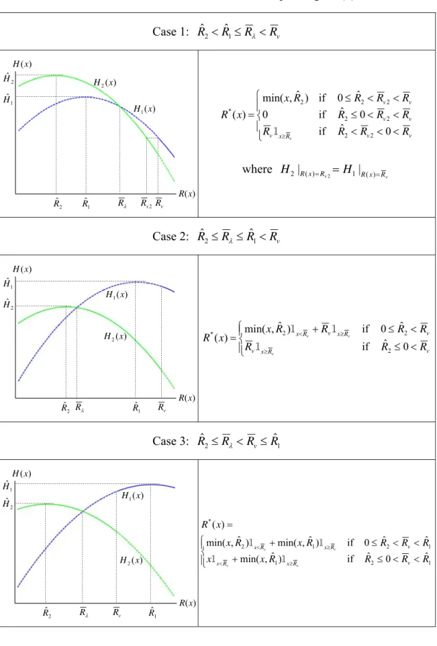
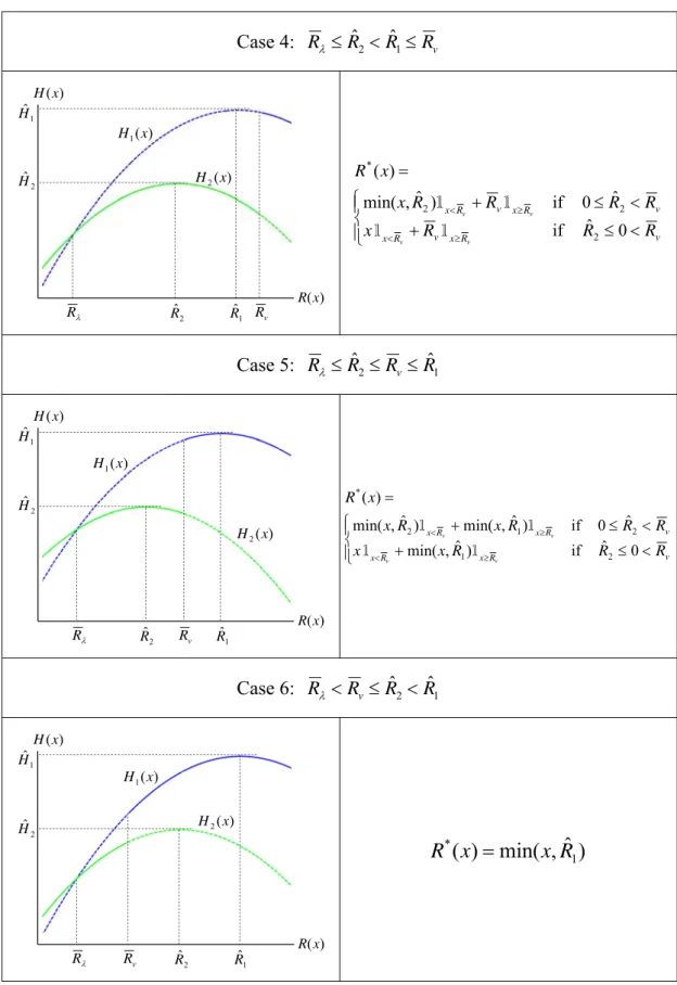
the thresholds   R   R R R R   ₂/ ₃ and VaR _v (35) where  R x R x H H₁ ₂( ) if ( ) (36)

The Hamiltonian has four critical points, ˆR , ₁ ˆR , ₂ R and _ R . Since _v Rˆ₂  Rˆ₁

and RRv, the four critical points have six different permutations. Table 1 presents the Hamiltonians and their optimal corresponding retained loss schedule *( )

x

respect to different cases. This study only considers the six cases. However, H₁(x)

and H₂(x) may form different patterns when they further move up, down, left and

right. For completeness, moreover, we must additionally consider the situations of

0

2 

 (VaR constraint unbinding) and ₃ 0 (CVaR constraint unbinding). These situations will be remained to future works.

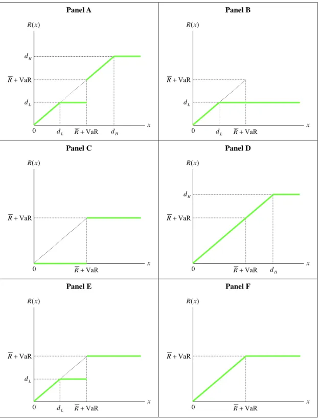
Based on Table 1, there are totally six different contractual forms shown on Table 2. Meanwhile, the representative contractual form is a double deductible insurance shown on Panel A. This result is similar to that in Huang (2006). Panel B is a standard deductible insurance in which both the constraints of VaR and CVaR are unbinding. And, Panel B contains the no insurance case of d_L0 or R(x) 0x. Besides

Panel B, the remained four contracts can be viewed as the degenerated form of Panel A, as follows.                      H L H L H L d R d R d R d R d d VaR if F Panel A Panel VaR if E Panel A Panel VaR if D Panel A Panel VaR and 0 if C Panel A Panel (37)

If the constraint (27b) is relieved, the above optimal insurance problem is reduced to the follows.

))] ( ( [ Maximize ₁ ) ( 0R xx E U E PR X (38) subject to 1( ) P h R x   (38a) E[R(X)R|R(X)R VaR]CVaR (38c) The solution process for equation (38) is similar but simple to Equation (27). The detail is remained to further work.

B. Insurer’s CVaR constraint

According to the assumptions and definitions in Section 2, the optimal insurance problem under the insurer’s CVaR constraint can be expressed as follows.

))] ( ( [ Maximize ₂ ) ( 0I x x E U E PI X (39) subject to 1( ) P h I   (39a)      VaR} 1 ) ( Pr{I X I (39b) E[I(X)I|I(X)I VaR]CVaR (39c) The corresponding Hamiltonian of the above program is

) ( CVaR)] ) 1 )( ) ( [( ) ( )] 1 ( [ ) ( ))] ( ) ( [ ) ( )) ( ( { VaR ) ( 3 VaR ) ( 2 1 1 2 x f I x I x f x f P h x I x f x I P E U H I x I I x I                  1 1     (40)

where ₁0, ₂ 0 and ₃0 represent the Lagrangean multiple coefficients. For simplicity, the Hamiltonian is redefined the following equation which has the same solution of I(x) as Equation (40).

) ( ]} ) 1 )( ) ( [( ) ( )) ( ( {U E₂ P I x ₁I x _{2 ( ) VaR 3} I x I _{( ) VaR} f x H      _{1I xI}   _{1I xI} (41)

Substituting E₁P , )I(x and I for E₂P , )R(x and R , Equation (41) is

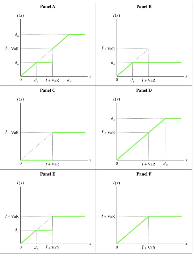
equivalent to Equation (31). This fact indicates that the solution of I(x) for maximizing Equation (41) is analogous to the solution of Equation (31). Accordingly, like Table 2, Table 3 display six different contractual forms of *( )

x

I .

If the constraint (39b) is relieved, the above optimal insurance problem is reduced to the follows.

))] ( ( [ Maximize ₂ ) ( 0 , 0   E U E PI X  (42)

subject to ( ) 1( ) P h I P I h     (42a) CVaR VaR] ) ( | ) ( [I X I I X I   E (42a)

Compared Equation (42) with Equation (22), we find the above optimal insurance problem resembles the problem in Zhou and Wu (2008). The solution process for equation (42) is similar but simple to Equation (39). The detail is remained to further work.

C. Optimal insurance premium and critical points

Following Raviv (1979) and Gollier (1987), the insurance problem is solved via two steps. First, given a fixed premium P, we solve the optimal indemnity

) ; ( * P x I

I  as a function of P. The second step determines the optimal insurance

premium *

P . The insurance contractual forms have been developed in the above

subsections A and B. Thus, this study proceeds to find the optimal premium. Since the two deductibles dL and dH depend on P, this study firstly finds the two deductibles as the premium function, dL dL(P) and dH dH(P). Since the calculation process of the optimal P for Table 3 is similar to Table 2, this study only presents the calculation for Table 2. Additionally, the insurance premium can be solved via the relation Ph(xR). This also presents that the critical point R VaR can be

directly found via P.

First, we can directly find the insurance premium P for Panel C and Panel F, as follows. R x dx x f R x R R R C



      [ ( VaR)] ( ) arg VaR (43) R x dx x f R x dx x f x R R R R F 







       ) ( )] VaR ( [ ) ( arg VaR VaR 0 (44)

Based on R and _C R , we obtain _F P_C h(xR_C) and P_F h(xR_F). Note that

D F E P P

P

P_C    and P_B P_F. Next, using the premium formula Ph(xR) can

find the critical points d_L d_L(P) in Panels B and d_H d_H(P) in Panel D. However,

besides RVaR, Panel A has two critical points d_L and d_H, indicating that the

calculation process for Panel A is more complicated than the others. Accordingly, the first step finds dH dH(dL,P) as a function of dL and P, using the premium principle Ph(xR). Subsequently, maximizing the insurer’s expected utility finds

) (P d

dL L and hence dH dH(dL)dH(P). Once all the critical points in Table 2 are represented as a function of P, maximizing the insurer’s expected utility with respect to P by common calculus can obtain the optimal premium *

P and the

corresponding six contractual forms. Nevertheless, *

P should meet the VaR and

CVaR constraints. Since Panels B, C, E and F never violate the CVaR constrict, the check of CVaR constraint focuses only Panel A and D. Finally, comparing the expected utilities among the six insurance contracts can elect the “exactly” and “uniquely” optimal insurance contract.

Table 1: The Hamiltonians and their corresponding *( ) x R Case 1: Rˆ₂Rˆ₁R_ R_v ) (x R ) (x H 1 ˆR 2 ˆR R Rv 1 ˆ H 2 ˆ H _{( )} 2 x H ) ( 1 x H 2 v R                R v v x v v v v v R R R R R R R R R R R x x R v 0 ˆ if 0 ˆ if 0 ˆ 0 if ) ˆ , min( ) ( 2 2 2 2 2 2 2 * 1 where v v R x R R x R H H₂ | _{( )}  ₁| _{( )} 2 Case 2: Rˆ2R Rˆ1Rv ) (x R ) (x H 1 ˆR 2 ˆR R Rv 2 ˆ H 1 ˆ H ) ( 2 x H ) ( 1 x H              v R x v v R x v R x R R R R R R R x x R v v v 0 ˆ if ˆ 0 if ) ˆ , min( ) ( 2 2 2 * 1 1 1 Case 3: Rˆ₂R_ R_vRˆ₁ ) (x R ) (x H 1 ˆR 2 ˆR R Rv 2 ˆ H 1 ˆ H ) ( 2 x H ) ( 1 x H                  1 2 1 1 2 1 2 * ˆ 0 ˆ if ) ˆ , min( ˆ ˆ 0 if ) ˆ , min( ) ˆ , min( ) ( R R R R x x R R R R x R x x R v R x R x v R x R x v v v v 1 1 1 1

Table 1: The Hamiltonians and their corresponding *( ) x R (continued) Case 4: R_ Rˆ₂ Rˆ₁R_v ) (x R ) (x H 1 ˆR 2 ˆR Rv  R 1 ˆ H 2 ˆ H H2(x) ) ( 1 x H                v R x v R x v R x v R x R R R x R R R R x x R v v v v 0 ˆ if ˆ 0 if ) ˆ , min( ) ( 2 2 2 * 1 1 1 1 Case 5: R_ Rˆ₂ R_vRˆ₁ ) (x R ) (x H 1 ˆ R 2 ˆR Rv  R 1 ˆ H 2 ˆ H ) ( 2 x H ) ( 1 x H                v R x R x v R x R x R R R x x R R R x R x x R v v v v 0 ˆ if ) ˆ , min( ˆ 0 if ) ˆ , min( ) ˆ , min( ) ( 2 1 2 1 2 * 1 1 1 1 Case 6: R_ R_vRˆ₂Rˆ₁ ) (x R ) (x H 1 ˆR 2 ˆR v R  R 1 ˆ H 2 ˆ H H2(x) ) ( 1 x H ) ˆ , min( ) ( ₁ * R x x R 

Table 2: Optimal contractual forms of *( )

x

R for insured’s CVaR constraint

Panel A x ) (x R H d VaR  R L d VaR  R 0 H d L d Panel B x ) (x R VaR  R L d VaR  R 0 L d Panel C x ) (x R VaR  R VaR  R 0 Panel D x ) (x R H d VaR  R VaR  R 0 H d Panel E x ) (x R VaR  R L d VaR  R 0 L d Panel F x ) (x R VaR  R VaR  R 0

Table 3: Optimal contractual forms of *( )

x

I for insured’s CVaR constraint

Panel A x ) (x I H d VaR  I L d VaR  I 0 H d L d Panel B x ) (x I VaR  I L d VaR  I 0 L d Panel C x ) (x I VaR  I VaR  I 0 Panel D x ) (x I H d VaR  I VaR  I 0 H d Panel E x ) (x I VaR  I L d VaR  I 0 L d Panel F x ) (x I VaR  I VaR  I 0

5. Conclusions

We have developed the optimal insurance forms under the insured’s and the insurer’s CVaR constraints, respectively, assuming that the insured is risk averse and the insurance premium is a function of expected indemnity. Nevertheless, the CVaR value is based on the calculated VaR value. So, the CVaR constraint frequently accompanies the VaR constraint. Consequently, the developed insurance contacts simultaneously meet the VaR and CVaR constraints. The main findings are as follows.

First, the insurance contractual forms with the insured’s VaR and CVaR constraints are analogous to the insurer’s ones. Second, the possible contracts have six different forms, including three single deductible insurances and three double

deductible insurances. Meanwhile, the three double deductibles contain one standard

form like the result in Huang (2006), and the remained two insurances are viewed as the degenerative forms. Third, one of the six insurances is a standard deductible insurance where the VaR and CVaR constraints are not binding. Besides the standard deductible insurance, the representative indemnity schedule has two deductibles, where the lower and the higher are respectively below and above a particular threshold (expected indemnity plus VaR). Moreover, the remained four contractual forms are the degenerative forms of the representative double deductible insurance.

The future works can consider the following directions. First, the utility function and loss probability distribution are further specified. This leads to an explicit insurance form. Next, besides the optimal contractual form, one can further determine the optimal coverage levels on the specific insurances including the proportional

coinsurance, deductible insurance, upper-limit insurance. Finally, comparing our

Reference

Acerbi C, Tasche D, 2002, On the coherence of expected shortfall, Journal of Banking

& Finance 26, 1487-1503.

Alexander GJ, Baptista AM, Yan S, 2007, Mean-variance portfolio selection with 'at-risk' constraints and discrete distributions, Journal of Banking & Finance 31, 3761-3781.

Alexander S, Coleman TF, Li Y, 2006, Minimizing CVaR and VaR for a portfolio of derivatives, Journal of Banking & Finance 30, 583-605.

Andersson F, Mausser H, Rosen D, 2001, Credit risk optimization with Conditional Value-at-Risk, Mathematical programming 89, 273-291.

Basak S and Alexander S, 2001, Value-at-Risk-Based risk management: optimal policies and asset prices, Review of Financial Studies 14, 371-405.

Cai J, Tan KS, Weng C, and Zhang Y, 2008, Optimal reinsurance under VaR and CTE risk measures, Insurance Mathematics & Economics 41, 185-196.

Doherty, NA and Schlesinger H, 1983, Optimal insurance in incomplete markets,

Journal of Political Economy 91, 1045−1054.

Ermoliev YM and Flam SD, 2001, Finding pareto optimal contracts, The Geneva

Papers on Risk and Insurance Theory 26, 155−167.

Gollier C, 1987, The design of optimal insurance contracts without the nonnegativity constraint on claims, Journal of Risk and Insurance 54, 314−324.

Gollier C, 1996, Optimal insurance of approximate losses, Journal of Risk and

Huang HH, 2006, Optimal insurance contract under value-at-risk constraint, The

Geneva Risk and Insurance Review 31, 91-110.

Jorion P, 2009, Value at Risk: the new benchmark for managing financial risk, 3/e,

McGraw-Hill International Edition.

Kibzun AI, Kuznetsov EA, 2006, Analysis of criteria VaR and CVaR, Journal of

Banking & Finance 30, 779-796.

Kuan CM, Yeh JH, Hsu YC, 2009, Assessing value at risk with CARE, the conditional autoregressive expectile models, Journal of Econometrics 150, 261-270.

Markowitz H, 1952, Portfolio Selection, Journal of Finance 7, 77-91. Morgan, JP, 1994, RiskMetrics, New York, October and November 1995.

Quaranta AG, Zaffaroni A, 2008, Robust optimization of conditional value at risk and portfolio selection, Journal of Banking & Finance 32, 2046-2056.

Raviv A, 1979, The design of an optimal insurance policy, American Economic

Review 69, 84−96.

Rockafellar RT, Uryasev S, 2002, Conditional value-at-risk for general loss distributions, Journal of Banking & Finance 26, 1443-1471.

Sun LH, Hong LJ, 2010, Asymptotic representations for importance-sampling estimators of value-at-risk and conditional value-at-risk, Operations Research

Letters 38, 246-251.

Szegö, G., 2005, Measures of risk, European Journal of Operational Research, 163, 5−19.

Tasche D, 2002, Expected shortfall and beyond, Journal of Banking & Finance 26, 1519-1533.

Topaloglou N, Valadimirou, Zenios SA, 2002, CVaR models with selective hedging for international asset allocation, Journal of Banking & Finance 26, 1535-1561. Vercammen J, 2001, Optimal insurance with nonseparable background risk, Journal

of Risk and Insurance 68, 437−448.

Wang CP, Shyu D, Huang HH, 2005, Optimal insurance design under a value-at-risk framework, The Geneva Risk and Insurance Review 30, 161-179.

Zhou CY, Wu CF, 2008, Optimal insurance under the insurer's risk constraint,

Insurance Mathematics & Economics 42, 992-999.

Zhou CY, Wu CF, 2009, Optimal Insurance Under the Insurer's VaR Constraint, The

Geneva Risk and Insurance Review 34, 140-154.

Zhou CY, Wu WF, Wu CF, 2010, Optimal insurance in the presence of insurer's loss limit, Insurance Mathematics & Economics 46, 300-307.

Zhou CY, Wu CF, Zhang SP, Huang X, 2008, An optimal insurance strategy for an individual under an intertemporal equilibrium, Insurance Mathematics &

Economics 42, 255-260.

Zhuang W, Chen Z, Hu T, 2009, Optimal allocation of policy limits and deductibles under distortion risk measures, Insurance Mathematics & Economics 44, 409-414.

國科會補助計畫衍生研發成果推廣資料表

日期:2012/10/23

國科會補助計畫

計畫名稱: 條件風險值限制下之最適保險契約 計畫主持人: 汪青萍 計畫編號: 100-2410-H-151-013- 學門領域: 財務

無研發成果推廣資料

100 年度專題研究計畫研究成果彙整表

計畫主持人：汪青萍 計畫編號： 100-2410-H-151-013-計畫名稱：條件風險值限制下之最適保險契約 量化 成果項目 實際已達成 數（被接受 或已發表） 預期總達成 數(含實際已 達成數) 本計畫實 際貢獻百 分比 單位 備 註 （ 質 化 說 明：如 數 個 計 畫 共 同 成 果、成 果 列 為 該 期 刊 之 封 面 故 事 ... 等） 期刊論文 0 0 100% 研究報告/技術報告 0 0 100% 研討會論文 0 0 100% 篇 論文著作 專書 0 0 100% 申請中件數 0 0 100% 專利 已獲得件數 0 0 100% 件 件數 0 0 100% 件 技術移轉 權利金 0 0 100% 千元 碩士生 2 2 100% 博士生 0 0 100% 博士後研究員 0 0 100% 國內 參與計畫人力 （本國籍） 專任助理 0 0 100% 人次 期刊論文 0 0 100% 研究報告/技術報告 0 0 100% 研討會論文 0 0 100% 篇 論文著作 專書 0 0 100% 章/本 申請中件數 0 0 100% 專利 已獲得件數 0 0 100% 件 件數 0 0 100% 件 技術移轉 權利金 0 0 100% 千元 碩士生 0 0 100% 博士生 0 0 100% 博士後研究員 0 0 100% 國外 參與計畫人力 （外國籍） 專任助理 0 0 100% 人次

其他成果

(

無法以量化表達之成 果如辦理學術活動、獲 得獎項、重要國際合 作、研究成果國際影響 力及其他協助產業技 術發展之具體效益事 項等，請以文字敘述填 列。) 無 成果項目 量化 名稱或內容性質簡述 測驗工具(含質性與量性) 0 課程/模組 0 電腦及網路系統或工具 0 教材 0 舉辦之活動/競賽 0 研討會/工作坊 0 電子報、網站 0 科 教 處 計 畫 加 填 項 目 計畫成果推廣之參與（閱聽）人數 0

國科會補助專題研究計畫成果報告自評表

請就研究內容與原計畫相符程度、達成預期目標情況、研究成果之學術或應用價

值（簡要敘述成果所代表之意義、價值、影響或進一步發展之可能性）

、是否適

合在學術期刊發表或申請專利、主要發現或其他有關價值等，作一綜合評估。

1. 請就研究內容與原計畫相符程度、達成預期目標情況作一綜合評估

■達成目標

□未達成目標（請說明，以 100 字為限）

□實驗失敗

□因故實驗中斷

□其他原因

說明：

2. 研究成果在學術期刊發表或申請專利等情形：

論文：□已發表 ■未發表之文稿 □撰寫中 □無

專利：□已獲得 □申請中 ■無

技轉：□已技轉 □洽談中 ■無

其他：（以 100 字為限）

3. 請依學術成就、技術創新、社會影響等方面，評估研究成果之學術或應用價

值（簡要敘述成果所代表之意義、價值、影響或進一步發展之可能性）（以

500 字為限）

最適保險研究為保險經濟領域重要議題之一，而且風險值與條件風險值的限制乃為金融業 重要風險控管指標，在金融與監理實務上非常重要，保險契約本為風險控管重要工具之 一，因此本文首先開發出同時受風險值與條件風險值限制下之最適保險契約，以供學術與 實務參考。本研究分別導出在被保險人或保險人受條件風險值限制下之最適保險契約。但 在實務上，條件風險值乃根據風險值算出，故條件風險值之限制經常伴隨著風險值之限 制。因此，本研究所導出的最適保險契約同時加入風險值與條件風險值的限制。研究結果 發現無論是被保險人或保險人受限於風險值與條件風險值，兩者之最適保險型式皆類似。 其次，最適保險契約可分為兩種類別。其一為不受到風險值與條件風險值限制的標準自負 額保險；另外為雙重自負額保險及其四種退化型式。