Clustering Gene Expression Time Series Data

全文

(1)Int. Computer Symposium, Dec. 15-17, 2004, Taipei, Taiwan.. Clustering Gene Expression Time Series Data Cheng-Che Wu1, Chun-Nan Kuo1, Jen-Peng Huang2, Huang-Cheng Kuo1* 1 Department of Computer Science and Information Engineering National Chiayi University 2 Department of Information Management Southern Taiwan University of Technology *[email protected] Abstract Efficiently and effectively finding the genes with similar behaviors from microarray data is an important task in bioinformatics community. Co-expression genes have the same behavior or are controlled by the same regulatory mechanisms. Clustering analysis is a very popular technique to group the co-expressed genes into the same cluster. One of the key issues for clustering gene expression time series data is to define the similarity between two time series. Distance measurements and correlation coefficients are commonly used similarity definitions. Two time series might be very distant, but they might be similar if a few items are dropped off from one of the two time series. In this paper, we consider this new aspect of time series similarity, denoted “shift effect,” which indicates temporal gap between two time series. For partition based clustering methods, users have to specify the target number of clusters. This is usually done by means of try-and-error to pick up a number from a large range. In order to solve this problem, we apply sequential pattern mining technique by treating time series as sequences. The number of frequent patterns is the number of target clusters. All the time series supporting a sequential pattern are the initial members of a cluster. Then, each time series is iteratively re-assigned to a suitable cluster. Keywords: microarray, gene expression, time series, clustering analysis. 1. Introduction Adapt to the genome sequences of human is defined, what we want to know urgently is how to annotate the information of DNA sequence, which is called gene annotation. There are about forty thousand functional genes in human genome, and these functional genes control the biochemical phenomenon of heredity, growth, and disease. This work is supported partially by National Science Council of Taiwan under grants NSC 93-2213-E-415-005, and NSC 93-2815-C-415-002-E.. Among these functional genes, a large number of them have not been discovered the functionalities. For this reason, the researches of probing gene functionalities will be very important and an urgent demand in bioinformatics in the future. Many analysis tools help biologists to discover co-expressed genes. During these tools, Microarray which is the most familiar tool helps to do the work. In once Microarray experiment, about 40,000 genes from 10 samples under 20 different conditions can be experimented. The result of Microarray experiments is an image data and it is scanned and transferred into numeric data which called expression levels. The data of several the same Microarray experiments with the same samples under different time points forms gene expression time series data. The data format of gene expression time series data is expressed as table 1. We will apply our clustering algorithm on gene expression time series data, and groups the co-expressed data in the same clusters. These clusters will help biologists to probe the relation between genes and physiological reactions. The partition-based iterative clustering method we addressed is divided into three parts: First, data preprocessing, second clusters adjusting, and third stop criterion checking. Each time series is discretized and translated into a sequence. Frequent patterns of the gene expression time series data set are found by mining frequent patterns. And then, let the set of time series which support the same pattern be grouped into the same cluster. For each time series in the data set, the nearest neighbors of the time series are found and to decide if it will be re-assigned to another cluster which the most nearest neighbors belong to. At last, checks if no time series is re-assigned to another cluster and terminate the clustering algorithm. It means that the clusters are stable.. 2. Related Work Frequent pattern mining [AS95] is based on association rule mining. It is the mining of frequently occurring patterns related to time or other sequences. Frequent patterns help to analysis the relationship of. 1192.

(2) Int. Computer Symposium, Dec. 15-17, 2004, Taipei, Taiwan.. events at different time points. Clustering is the process of grouping data with similar character into the same class or the same cluster. The character of clustering is that objects in the same cluster have high similarity and objects in the different clusters have low similarity. Clustering is also an important analysis technique in bioinformatics recently. Traditional clustering techniques can be distinguished as three common types which are partition-based clustering methods, hierarchical clustering methods, and density-based clustering methods. These clustering methods have been applied to cluster gene expression time series data. But, there are still some problems when clustering gene expression time series data using traditional clustering methods [JPZ03]. In partition-based clustering such as K-means [THC99] and SOM [TSM99], the users are requested to give the number of clusters. The result of clustering gene expression data is usually unable be forecasted. The parameter of the number of cluster may decrease the accuracy of the result of clustering. And another issue of partition-based clustering is that most algorithms use distance-based measure metrics and lead to the sphere shape clusters. In hierarchical clustering such as CURE [GRS98] and ROCK [GRS99], the result of clustering forms a hierarchical structure, called dendrogram. It is a difficult problem to decide where to cut the dendrogram and get the suitable clusters. Expert domain knowledge usually helps to do it. In hierarchical clustering, two elements are jointed based only on the distance measurement of the elements. When elements are joined, they could not be separated anymore, and it will lead the clustering process to a wrong way. Another drawback of hierarchical clustering is that the inner structure of clusters is usually unintelligible. In density-based clustering such as DBSCAN [EKS96] is quite sensitive to the parameters of time series density. These parameters are used to be thresholds that if a time series is one of cores of a cluster. The suitable parameters are hard to resolve in a complex data set. The noises of data sets are usually distributed randomly, and the density within clusters must be obvious higher than the density of the outlier. For the reason, density-based clustering is suitable to highly noisy data sets such as the case of gene expression time series data sets.. In this paper, we overcome the challenge of partition-based clustering. The initial clusters are generated by mining frequent patterns in our method. Genes with similar tendency are grouped first and each cluster is formed according to the characteristic of genes. It is more confident for clustering.. 3. Motivation Although many traditional clustering methods had applied to gene expression time series data, several challenges were generated as above. How to cluster gene expression time series data efficiently and accurately is an important task for bioinformatics. Gene expression time series data clustering should tolerant both biological variances and non-biological noises. The accuracy of the result of time series clustering based on the similarity measurement. Common used similarity definitions such as distance measurement and coefficient measurement can not be applied on measuring the similarity between time series straight. In many cases, time series with sift effect exist in the data and the common used similarity definitions could not solve the problem of shift effect. We apply a mixed similarity function for gene expression time series similarity. The clustering algorithm we addressed is based the nearest neighbors and the result of clustering would not lead to the sphere shape clusters. We expect that it will improve the accuracy of the result of gene expression time series clustering.. 4. The Algorithm of KNN Clustering 4.1. Data preprocessing In order to mine the patterns of gene expression time series data, each time series must be translated as a sequence. The changes of consecutive time points during the time series are expressed as symbols in sequence. Let T = t1 , t 2 , t3 , " , t n be. {. a time series with length n, σ T and η T be the standard deviation and mean value of time series T. Before discretizing the time series T, normalization of each time series helps to exclude the effects of scalability and offset. Each element t i of time series T is normalized as. Table 1: Format of gene expression time series data YORF Gene 1 Gene 2 Gene 3. … … … …. Time point m -0.02 -0.34 0.21. t i′ =. ti − ηT. σT. , 1≤ i ≤ n .. A normalized time series T ′ = {t1′ , t 2′ , t 3′ ,", t n′ } can. transformed S = {s1 , s 2 , " , s n −1 } as. be. into. a. sequence. ⎢ t′ − t′ ⎥ si = ⎢ i +1 i ⎥ , 1 ≤ i ≤ n − 1 . ⎣ σT ⎦. …. 0.22. …. …. 0.08. Time point 2 0.11 0.02 0.33 …. …. … Gene n. Time point 1 0.23 -0.17 0.69. }. -0.01. 1193.

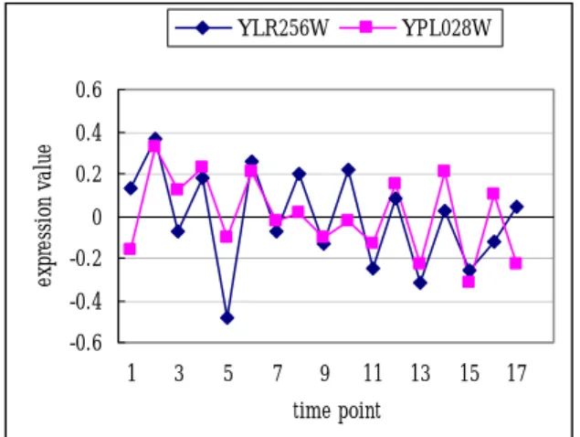
(3) Int. Computer Symposium, Dec. 15-17, 2004, Taipei, Taiwan.. σT. is used to determine the. 0.6. G1 G2 G3. Sequence. (0.21, 0.35, 0.89, 0.34, 0.11). (0, 3, -4, -1). (-0.2 ,0.11 ,0.03, 0.22, -0.13). (3, 0, 2,-4). (0.97, 0.38, -0.14, -0.91, 0.01). (-1, -1, -2, 1). …. …. …. Gn. (0.11, 0.15, 0.47, 0.65, 0.92). (0, 1, 1, 1). 0.4 0.2 0 -0.2 -0.4 -0.6 1. 3. 5. 7. 9. 11. 13. 15. 17. time point. Figure 1: Two time series profiles having large Euclidean distance Another issue is produced in generating initial clusters by mining frequent patterns. There may be several genes support not only one frequent pattern. Patterns may be supported by partial the same genes and form intersected clusters. In clustering, a time series can exist in just one cluster. For the reason, a gene which supports several patterns can be just assigned into one cluster. A solution is that the gene is assigned into the cluster which has the maximum length of frequent pattern it supports. YLR256W. YPL028W. 0.6. Table 2: Transferred time series into sequences Time series. YPL028W. YLR256W. expression value. degree of the significant change between the consecutive time points. The large change between the consecutive time points during the time series express a large value in the sequence. There is an example illustrates as table 2. After all the time series in the data set are transformed into sequences and forms a sequence data set. Several frequent patterns are generated by mining frequent pattern on the data set. For some sequences which support no frequent patterns are not considered at the procedure of clustering, and the sequences may be meaningful for researches. These frequent patterns are regarded as initial clusters. Genes support the same frequent pattern mean that they have portions of similar expressions, and a high possibility indicates that they may be assigned to the same cluster. A special case that can not be solved by many clustering methods depend on Euclidean distance is time series with similar profiles have long Euclidean distance. Two time series have similar profile but having a temporal offset should be considered similar and belonged to the same cluster in bioinformatics. But, the distance between the time series measured by Euclidean distance is a long distance, and they may be distributed into different cluster. The problem occurred base on the definition of similarity. The time series with “shift effect” are illustrated in Figure 1. The Euclidean distance of YLR256W and YPL028W is 1.483, and the value of correlation coefficient between YLR256W and YPL028W is -0.509. But, we will get high similarity of the two time series after deleting the last point of YLR256W and the first point of YPL028W, and then let YPL028W be shifted one time point left. The time series are illustrated in Figure 2. After processing, the Euclidean distance of YLR256W and YPL028W is 0.792, and the value of correlation coefficient between YLR256W and YPL028W is 0.623. The similarity between YLR256W and YPL028W increases greatly.. as the definition of similarity. Some time series with similar profiles may indicate that they have high similarity. But, due to the influence of shift effect, the time series have large Euclidean distances between them. Therefore they may be assigned to different clusters at last. After some elements of these time series are removed, we can find that they have small Euclidean distances. This is an issue in clustering gene expression time series data.. expression value. The threshold. 0.4 0.2 0 -0.2 -0.4 -0.6 1. 3. 5. 7. 9. 11. 13. 15. 17. time point. Figure 2: Two time series after excluding shift effect. Because the greater part of clustering methods apply to cluster time series may defined the similarity first. Before the similarity is defined, the regulation of scaling, base line shifting, and offset handling were be finished, and then use the Euclidean distance. 4.2. Adjusting clusters When each time series is assigned into only one cluster, the next step is to adjust the clusters. It. 1194.

(4) Int. Computer Symposium, Dec. 15-17, 2004, Taipei, Taiwan.. re-assigns a time series from a cluster to another if the later cluster is more suitable for the time series. It is an iterative procedure to re-assign time series into the most suitable clusters. The nearest neighbors of time series are used as the basis of time series re-assignment. The detail description will be stated in next section. The procedure will stop until all of the clusters are static. During the step below, we just consider the time series suppose at least one frequent pattern. In the next section, we will first define a similarity metric for the similarity measurement of time series and explain our proposed clustering algorithm.. 4.3. Similarity definition Before adjusting the clusters, similarity metric must be defined first. The similarity metric is one of the major factors of accuracy for time series clustering. There are some issues for measuring similarity between time series such as scalability, baseline offset, outliers, and shift effect. None of the common used similarity definition could solve these issues simultaneously. At another viewpoint, what we concerned with not only the intensity of expression but also the time points which are inducement or restraint. In this paper, we define the similarity metric by collocating common used similarity metrics. One of the similarity metrics we used is standard correlation coefficient. The similarity between two time series X , Y of length n was define as. ∑x y − ∑x ∑ y / n (∑x − (∑x ) / n)(∑ y − (∑ y ) / n). r( X , Y ) =. i i. 2 i. i. 2. i. i. series X = { x1 , x2 ," , xn } , Y = { y1 , y2 ," , yn }. was define as LCSL( X , Y ) which is the ratio of the greater part common similar expression level of X and Y of length n [DGM96]. The longest common subseries are explored as bellow:. (1 + ε ). LCSS ( X , Y ) n. LCSL can clearly indicate the degree of common expression portions but not concern the intensity of expression level. Based on the characteristic of correlation coefficient and LCSL, the value of correlation coefficient of X and Y is normalized and denoted as r ′( X , Y ) first. Lastly, we integrate both similarity metrics and define the similarity of time series X and Y as:. sim ( X , Y ) = w1 × r ′ ( X , Y ) + w2 × LCSL ( X , Y ) In the equation, w1 and w2 are the weights of both similarity metrics. The definition of similarity takes both the intensity of expression level and the degree of common expression portions into account. It may be more suitable for gene expression time series clustering.. 2. The value of r ( X , Y ) is between 1 and -1. The correlation coefficient is known to have good results in clustering and analyzing time series [ESB98]. But correlation coefficient may not get the similarity when two time series with shift effect. For the reason, we cooperate with another similarity metric to improve the defect. Another similarity metric we used is Longest Common Subseries Length (LCSL) [RCL01]. Two time series with the greater part similar expression levels could get high similarity calculated by LCSL. The distance between two time. yj. LCSL( X , Y ) =. 4.4. KNN clustering. i. 2 i. Two time points x and y are considered to be the same only when the difference between x and y is not over the multiple of ε. According to the definition, the longest common subseries of two time series can be explored. Let LCSS(X,Y) be the length of the longest common subseries of time series X and time series Y with length n and the similarity of X and Y is denoted as LCSL(X, Y).. ≤ xi ≤ y j (1 + ε ) , 1 ≤ i, j ≤ n. where, εis a parameter which is between zero and 1.. After generating the initial clusters, the vantage point of each cluster which likes centroid must be found for clustering first. The vantage point of one cluster represents a time series in the cluster. The vantage point is the time series which has the maximum sum of similarity with the rest time series in the cluster. During every iterative path, the vantage point of each cluster would be re-elected. KNN clustering is a partition based clustering. Rather than requesting users for the target number of clusters, the more confident clusters were generated by mining frequent patterns. Each initial cluster contains time series suppose the same expression pattern. The number of final clusters does not guarantee to be the same of the number of initial clusters. Some clusters may disappear when all of time series in the clusters are re-assigned to other clusters during the process of clustering. In KNN clustering, the k nearest neighbors of each time series must be found first for clustering. Which cluster one time series should be re-assigned bases on the distribution of the clusters nearest neighbors belong to. The k nearest neighbors of one time series may exist in several different clusters and the clusters are the candidate clusters that the time. 1195.

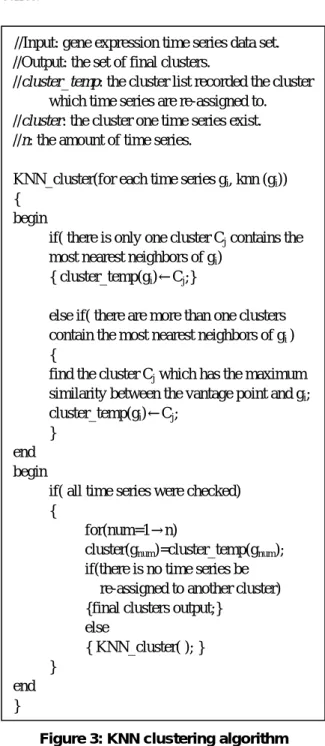
(5) Int. Computer Symposium, Dec. 15-17, 2004, Taipei, Taiwan.. series will re-assign to. There are two cases when one time series is re-assigned. First, there is only one cluster contains the most number of nearest neighbors of the k nearest neighbors. In the case, the time series will be re-assigned to the cluster contains the most nearest neighbors. The other case, there are more than one clusters contain the same and the most nearest neighbors of the k nearest neighbors. In this case, the similarities between the time series and the vantage points of all clusters with the most nearest neighbors will be calculated. The time series is re-assigned to the cluster with the maximum similarity between the vantage point and the time series. //Input: gene expression time series data set. //Output: the set of final clusters. //cluster_temp: the cluster list recorded the cluster which time series are re-assigned to. //cluster: the cluster one time series exist. //n: the amount of time series. KNN_cluster(for each time series gi, knn (gi)) { begin if( there is only one cluster Cj contains the most nearest neighbors of gi) { cluster_temp(gi)←Cj;} else if( there are more than one clusters contain the most nearest neighbors of gi ) { find the cluster Cj which has the maximum similarity between the vantage point and gi; cluster_temp(gi)←Cj; } end begin if( all time series were checked) { for(num=1→n) cluster(gnum)=cluster_temp(gnum); if(there is no time series be re-assigned to another cluster) {final clusters output;} else { KNN_cluster( ); } }. series which are re-assigned at this iteration, the stop criterion is set as false and the KNN clustering algorithm is restarted. The KNN clustering algorithm will be reiterated until no time series are re-assigned to another cluster. When all of the clusters were stable, the clusters are the result of gene expression time series clustering. The KNN clustering algorithm is described in Figure 3.. 5. Conclusion and Future Work Clustering is one of the most important techniques for finding the genes with the same expressions. Many traditional clustering methods help to cluster gene expression time series but they have several drawbacks and may not suitable. In this paper, we address a partition-based clustering algorithm and tie in frequent pattern mining to cluster gene expression time series data. The principal of our clustering method is to improve some challenges of traditional clustering methods. In our method, we define a combinative similarity metric that pay attention on both the intensity of expression level and the degree of common expression portions. Another improvement is that the number of target clusters are generated meaningfully, and users don’t have to predict how many clusters may exist. Subsequently, the time series are trained and re-assigned to the suitable clusters. Therefore embedded clusters and highly intersect clusters can be handled efficiently. One case that many traditional clustering methods which depend on Euclidean distance can not solve is that time series with similar profile but have large Euclidean distances. For this case, the time series usually were assigned to different clusters by traditional clustering methods, and the problem can be improved in our algorithm. What we confer in the future is two parts. The first part is that for our similarity metric, if we can find suitable weights used for correlation coefficient and LCSL. It may let our similarity more suitable for gene expression time series clustering. The other one is that the frequent patterns were generated by requesting users to give the minimum supposes. In place of requesting the minimum supposes given by users, we want to discover a method to generate a suitable minimum suppose. And the method for generating minimum supposes will be suitable for use on different data sets.. References. end } Figure 3: KNN clustering algorithm When all of the time series are tested, the vantage point of each cluster is re-elected. Then the algorithm checks if the stop criterion is true. If there are time. [JPZ03] Daxin Jiang, Jian Pei, Aidong Zhang. “DHC: A Density-based Hierarchical Clustering Method for Gene expression time series data,” IEEE Symposium on Bioinformatics and BioEngineering, 2003.. 1196.

(6) Int. Computer Symposium, Dec. 15-17, 2004, Taipei, Taiwan.. [JPZ03] Daxin Jiang, Jian Pei, Aidong Zhang, “Interactive Exploration of Coherent Patterns in Time-series Gene Expression Data,” ACM SIGKDD, 2003. [AS95] Rakesh Agrawal, Ramakrishnan Srikant. “Mining Sequential Patterns,” International Conference on Data Engineering, 1995. [THC99] Tavazoie, S. et al. “Systematic determination of genetic network,” Architecture. Nature Genet, 1999. [TSM99] Tamayo P. et al. “Interpreting patterns of gene expression with self-organizing maps: Methods and application to hematopoietic differentiation,” Natl. Acad. Sci, 1999. [GRS98] Sudipto Guha, Rajeev Rastogi, Kyuseok Shim. “CURE: An Efficient Clustering Algorithm for Large Databases,”ACM SIGMOD International Conference on Management of Data, 1998. [GRS99] Sudipto Guha, Rajeev Rastogi, Kyuseok Shim. “ROCK: A Robust Clustering Algorithm for Categorical Attributes,” IEEE International Conference on Data Engineering, 1999. [EKS96] M. et al. Ester. “A Density-Based Algorithm for Discovering Clusters in Large Spatial Databases with Noise,” International Conference on KDD, 1996. [Aas01] Kjersti Aas. Microarray Data Mining: A Survey. Norsk Regnesentral, 2001. [EOA04] Selnur Erdal, Ozgur Ozturk, David Armbruster, Hakan Ferhatosmanoglu, William C. Ray, “A Time Series Analysis of Microarray Data,” IEEE Symposium on Bioinformatics and BioEngineering, 2004. [HB01] Bernard Hugueney, Bernadette Bouchon-Meunier, “Time-Series Segmentation and Symbolic Representation from Process-Monitoring to Data-Mining,” Lecture Notes in Computer Science, volume 2206, 2001. [RCL01] Ronald L. Riverst, Thomas H. Cormen, Charles E. Leiserson, Cliffod Stein, Introduction to algorithms, McGraw-Hill Book Company, 2001. [ESB98] M. B. Eisen, P. T. Spellman, P.O. Brown, D. Botstein, “Cluster analysis and display of genome-wide expression patterns,” National Academy of Science, 1998. [Dun02] Margaret H. Dunham, Data mining introductory and advanced topics, Prentice Hall, 2002. [FSZ01] Vladimir Filkov, Steven Skiena, Jizu Zhi. “Analysis Techniques for Microarray Time-Series Data,” International conference on Computational biology, 2001. [TWB03] Thanh N. Tran, Ron Wehrens, L.M.C. Buydens. “KNN density-based clustering for high-dimensional multispectral images,” GRSS/ISPRS Joint Workshop on Remote Sensing and Data Fusion over Urban Areas, URBAN 2003. [DGM96] Gautam Das, Dimitrios Gunopulos, Heikki Mannila. “Finding Similar Time Series,” Journal of Data Mining and Knowledge Discovery, 1996.. 1197.

(7)