SIGNAL
PROCESSING
ELSEVIER
Signal Processing 57 (1997) 177-194Adaptive beamforming with interpolated arrays for multiple
coherent interferers
Ta-Sung Lee*, Tsui-Tsai Lin
Department of Communications Engineering, National Chiao Tung University, Hsinchu. Taiwan Received 15 March 1996; revised 17 October 1996
Abstract
The spatial smoothing technique is effective in decorrelating multiple coherent interferers for an adaptive beamformer. However, it requires a configuration with identical subarrays. This paper presents an interpolation scheme to synthesize multiple virtual subarrays allowing for the use of spatial smoothing from a real array of arbitrary geometry. After interpolation, the optimum spatially smoothed subarray beamformer is constructed. A dimension recovery transformation can then be implemented to calculate the weights of the full array which will retain the interference nulls of the subarray beamformer. The efficacy of the proposed scheme is assessed through simulation. @ 1997 Elsevier Science B.V.
Zusammenfassung
Allgemein stellt die Technik der raumlichen Gl&ung bei Verwendung eines adaptiven Beamformers ein effizientes Mittel dar, um mehrere koharente Stijrquellen zu dekorrelieren. Allerdings wird hierbei eine Sensoranordnung benotigt, die aus identischen Sensorgruppen besteht. Dieser Artikel stellt ein Interpolationsverfahren vor, mit dessen Hilfe mehrere virtuelle Sensorgruppen synthetisiert werden konnen, so dal.3 die raumliche Gl&ung such bei Sensorgruppen beliebiger Geometrie angewandt werden kann. Nach der Interpolation wird der optimale raumlich gegliittete Untergruppenbeamformer konstruiert. Anschliegend kann eine Dimensions-Riickgewinnungstransfonnation implementiert werden, um die Gewichtsfaktoren fiir die gesamte Sensorgruppe zu berechnen. Dabei bleiben die Nullstellen im Diagramm des Untergruppenbeamformers an den Stijrpositionen erhalten. Abschlieljend wird die Wirksamkeit des vorgestellten Verfahrens anhand von Simulationen beurteilt. @ 1997 Elsevier Science B.V.
La technique de lissage spatial est efficace pour decorreler des signaux d’interference multiples coherents dans un formatteur de voie adaptatif. Toutefois, elle r&lame une configuration comprenant des sous-reseaux identiques. Cet article presente une methode d’interpolation pour synthetiser, a partir d’un reseau de geometric arbitraire, des sous-reseaux virtuels multiples permettant l’utilisation du lissage spatial. Apres interpolation, le formatteur de voie optimal du sous-reseau lisst spatialement est construit. Une transformation de recouvrement de dimension peut ensuite 8tre implant&e afin de calculer les pond&rations du reseau complet, qui conservera les zeros d’interference du formatteur de voie du sous-reseau. L’efficacite du schema propose est montree a I’aide de simulations. @ 1997 Elsevier Science B.V.
Keywords: Beamfooning; Array processing; Interpolation
* Corresponding author. Tel.: +886 35 712 121; fax: 886 35 710 116; e-mail: [email protected].
0165-1684197/$17.00 @ 1997 Elsevier Science B.V. All rights reserved. PZZSO165-1684(96)00194-6
178 T.-S. Lee, T-T. Lin / Signal Processing 57 (1997) 177-194
1. Introduction
An
adaptive beamformer performs spatial filtering by forming a beam in such a fashion that the desired signal can be received with a large gain, while un- desired interfering signals can be suppressed [6]. Conventional adaptive beamformers are found to be effective in suppressing strong interferers so long as the pointing error is negligible and the interferers are uncorrelated with the desired source. In the presence of pointing errors and/or correlated interferers, these beamformers exhibit degradation in performance in that the output signal-to-interference-plus-noise ratio (SINR) drops significantly. In some extreme cases, such as with large pointing errors or coherent inter- ference, the conventional beamformers break down as a result of desired signal cancellation. Remedies have been proposed to lessen the effect of desired signal cancellation [3,5, 111. In particular, the Duvall processor was suggested in Ref. [ 1 l] as a means of improving the robustness of an adaptive beamformer operating on an array with the ‘doublet’ structure, such as the uniform linear array (ULA). With the Duvall processor, the desired signal is first attenuated by using a subtractive preprocessor. The optimum weights are then calculated based on the preprocessed data. With this mode of operation, the beamformer will not cancel the desired signal, even in the pres- ence of pointing errors and coherent interference. We refer to this type of beamformers as the ‘suppressed- desired signal ’ (SD) beamformers.In spite of the success of dealing with pointing errors of moderate size and a single coherent inter- ferer, the Duvall beamformer still exhibits a certain degradation in the presence of large pointing errors or multiple coherent interferers [3,5,7]. With large pointing errors, the desired signal cannot be attenuated sufficiently such that a portion of its power will be eliminated by the beamformer. This problem can be lessened by using high order look direction constraints to broaden the effective region of desired signal atten- uation, or using some kind of algorithm to ‘track’ the desired source direction [3]. On the other hand, the difficulty incurred with multiple coherent interferers is a consequence of the fact that the relationship govem- ing the mutual cancellation of the interfering signals in the master beamformer is destroyed in the slave beam- former. A similar situation which is likely to happen
in a mobile scenario is that the relative phases of the coherent multipath signals change so rapidly that an adaptive beamformer is unable to keep up an effective mutual cancellation of these interferers. To avoid such degradation, the spatial smoothing technique [8] can be employed as a means of decorrelating the interfer- ers before the optimum weights are obtained [4,7,8]. This ensures that the beamformer will suppress the in- terferers individually, instead of performing a mutual cancellation. However, working with spatial smooth- ing requires an array consisting of spatially shifted identical subarrays, which may not be attainable in practice. A question then arises as to whether an adap- tive beamformer can be implemented on an arbitrary array to handle multiple coherent interferers. In [lo], an interpolation technique was proposed for trans- forming an arbitrary array into a ULA such that spatial smoothing can be applied to estimate the directions of coherent sources. Detailed discussions on the interpo- lation procedure are given in Ref. [l]. It was shown that an interpolated array can perform almost as well as a real array for source localization [ 11. Similar re- sults can be expected for adaptive beamforming.
This paper presents a beamforming scheme for combating multiple coherent interferers with an inter- polated array. The procedure consists of three steps. Firstly, spatially shifted identical virtual subarrays are synthesized from the same real array by linear interpolation [I]. Specifically, the interpolator is de- signed such that the interferers are transformed dis- tortionlessly onto the virtual subarrays, whereas the desired source is eliminated. The latter operation is similar to the subtractive preprocessing in the Duvall beamformer. Secondly, a spatially smoothed virtual subarray correlation matrix is formed, from which the optimum weight vector can be obtained to produce a null for each interferer. Finally, the subarray weight vector is converted back into a full aperture weight vector acting on the real array via a dimension re- covery transformation and post combining. Two dif- ferent combiners are suggested: the maximum output signal-to-noise ratio (SNR) combiner and the eigen- based combiner. The former is easier to implement, whereas the latter is more robust to pointing errors. The efficacy of the proposed beamformer is ascertained by several sets of numerical examples using the nonuniform linear array and circular array configurations.
T-S. Lee, T.-T Lin/Signal Processing 57 (1997) 177-194 179
2. Problem formulation
where2.1.
Notations A = wd), a@1 >, . . , +k)i, (2)and S = [s&s,, . . .,sK] T. The random scalars sd and Sk, k = I,..., K, represent the desired and interfer- ing signal samples received at the reference point of the array. The A4 x 1 vectors a(&) and a(&), k = 1,. . . , K, are the direction vectors accounting for the gain and phase variations across the array due to the desired and interfering signals from direction & and ek, k = 1,. . . , K, respectively. Finally, the vector n is composed of the noise components present at the M elements. The noise is assumed to be spatially white with power IJ~ and uncorrelated with the desired and interfering signals.
n x 1 zero vector
Euclidean norm expectation
desired source direction interfering source direction look direction
noise power normalizing scalar
primary interpolation region auxiliary interpolation region
interpolation region associated with desired signal
interpolation region associated with interfer- ence
parameter controlling the relative emphasis between the interpolation performance over 0 and 0,
wavelength
phase shift matrix associated with the ith subarray
phase shift between the ith and reference subarrays for direction 6’
normalizing scalar normalizing scalar generalized eigenvalue
deviation of interpolation region
Superscripts
T: transpose
H: complex conjugate transpose 2.2. Array model and beamforming
The scenario considered herein involves a single desired source and K possibly mutually correlated in- terferers, all assumed to be narrowband with the same center frequency. These sources are in the far field of an array consisting of M elements. Adopting the com- plex envelop notation, the array data obtained at a cer- tain sampling instant can be put in the A4 x 1 vector form:
(1)
A beamformer is a linear combiner which trans- forms the array data vector into a scalar y via an M x 1 complex weight vector W:
y = W”X. (3)
Associated with the beamformer constructed with w is the beam pattern defined by
w(e) = wHu(e),
(4)which describes the spatial response of the beam- former. The optimum beamformer which we will work with is constructed so as to minimize the output power subject to a unit response constraint in the look direc- tion
e.
:rn$r E { ly12> - wHRxxw
subject to wHa(BO) = 1, (5) where
R,
is the A4 x M data correlation matrix. In- voking the spatial whiteness of n and using (1 ), we haveR, =
E {xx”} =AR&”
+ o,2ZM,
(6)
where
R,, =
E{ssH} is the source correlation matrix,and
ZM
is the A4 x M identity matrix. The linearly constrained minimum variance (LCMV) problem [9] in (5) has the solutionW =
yR$u(B&
where y is a normalizing scalar.
180 T-S. Lee, T-T. Lin/ Signal Processing 57 (1997j 177-194
The optimum beamformer is known to perform poorly in the presence of pointing errors and/or co- herent interference. A subtractive preprocessor can lessen the problem incurred with pointing errors and a single coherent interferer, but cannot handle multiple coherent interferers. This prompts the development of a scheme to decor-relate the interferers before beamforming. For an array consisting of identical subarrays, the decorrelation can be done with spatial smoothing. When this is not the case, one must resort to the numerical approach, i.e., array interpolation, to reconfigure the array.
structure modified in a tolerable fashion, This issue will be discussed shortly.
The interpolation of virtual subarrays is performed in a linear fashion. That is, we use L transformation matrices 4, i = I,. . . , L, of size M, x M to transform the real array direction vector a(8) into the virtual subarray direction vectors Qt?), i = 1,. . . ,L, over a prescribed angular region 0 :
zU(O) = hi(S), 8 E 0, i = 1,. . . ,L. (8) Usually the interpolation region consists of several subregions around the hypothesized source directions obtained from the preliminary localization.
3.
Formation of the interpolated arrays
3.2. Suppressed-desired signal (SD) interpolators This section describes the procedure for formingthe interpolated array and discusses various issues on array interpolation. The procedure involves creating L spatially shifted identical virtual subarrays of M, elements from the real array.
3.1. Interpolation of virtual subarrays
As described earlier in Section 1, an effective way of avoiding desired signal cancellation due to point- ing errors is to remove the look direction signal before beamforming. The idea can be incorporated into the interpolation process by forcing the transformed di- rection vectors to be zero in the neighborhood of the look direction. That is, we define the modified trans- formation matrices Fi, i = 1,. . . ,L, such that There are two major considerations in designing
the interpolated array. Firstly, both the configuration of the virtual subarrays and angular region for inter- polation need be determined beforehand. Secondly, the original signal-noise condition should be retained on the interpolated array so as to ensure a reliable beamforming performance. In general, the virtual sub- arrays should have a similar ‘shape’ to that of the real array, and should span an overall aperture comparable to that of the real array so as to keep the interpola- tion error small. On the other hand, the size of each virtual subarray should be large enough to provide a sufficient degree of freedom for interference nulling. Nevertheless, the number of subarrays need not be large as the improvement in spatial smoothing bene- fited by a large L will be likely offset by the increased interpolation errors and computational complexity. To determine the angular region for interpolation, prelim- inary estimates of the source directions are necessary. They can be obtained by using a nonadaptive beam- former to scan over the spatial spectrum and locate the peaks. In order that the signal-noise condition does not change dramatically after interpolation, the source sig- nals should be transformed distortionlessly and noise
L
,**.,
9 (9)where we split @ into 0 = @n U 01, with @o denoting the interpolation region associated with the desired source, and 01 the interpolation region associated with the interference. For brevity of notation, we rewrite (9) as
f@(e) = ro(e)bi(e), 8 E 0, i = 1,. . . ,_& (10) where In(e) is the indicator function defined by
(11)
In general, the larger the angular region @o over which the zero forcing is performed, the more robust the beamformer will be against pointing errors. In the following development, we will work with Pi’s for beamforming and refer to them as the transformation matrices associated with SD type interpolator. The original form of I;:‘s will be employed later for the purpose of dimension recovery and will be referred to as the transformation matrices associated with regular type interpolator.
T.-S. Lee, T.-T. Lin/Signal Processing 57 (1997) 177-194 181
3.3. Solution of transformation matrices
Eqs. (8) and (9) do not hold in general, but can be
approximated by the least-squares (LS) problems:
(12)
and
mjn
s
I( fin
- Zn(0)6i(0)l12 de,
I 0
(13)
respectively, whose solutions are easily seen to be
given by
s
IS 1
-1 4 =bi(ejaH(e)de a(e
de
(14)
0
B
and
J
[J I
-1
E
= ZD(t?)bi(tQ2H(f3)
de a(e)aH(e)de
, 0 8 (15)respectively. These solutions may cause numerical
problems if the interpolation region is small. In this
case, the matrix
[J,u(0)uH(O)dO]-ltends to be ill-
conditioned, and the resulting transformation matrices
in Eqs. (14) and (15) will have very large entries.
This in turn results in an ‘enlarged’ virtual subarray
noise correlation matrix as will be seen later in (35).
As a result, the signal-noise condition will be dra-
matically distorted, and the beamformer may fail to
eliminate the interferers since they are no longer the
dominant sources.
The transformation matrices can be made better
conditioned by augmenting 0 with an extra interpola-
tion region 0~ covering a much wider angular range.
This leads to the modified problems corresponding to
Eqs. (12) and (13):
mrin
'Q
J
)I &z(e) - Si(0)l(2 de
+E
J
QA
(Ii%(B)
-
bi(e)/12
de
(16)
and
IT$II
I
J
Q
Ilfia(e) -
Z0(e)bi(Ql12de
+E
J
@A
1)
Es(e)
- bi(e)l12
de,
(17)
where E is a parameter controlling the relative em-
phasis between the interpolation performance over the
primary (0) and auxiliary (@A) regions. Accordingly,
the resulting solutions are given by
F=
[J
bi(@uH(0)d6’
+
E0
J
bi(QaH(0)
df3 P,-’
@A
1 (18)
and
j+
[J
zD(tl)bi(0)aH(tl)
de+&
bi(0)aH(O) de pE_l,
0
J
@A
1
(19)
where
p, =
J
8
a(e
de + E
J
@A
a(e
de.
(20)
3.4. Issues
on interpolation processAugmenting the interpolation region with @A in
Eqs. (18) and (19) will not only alleviate the ill-
condition problem, but also improve the robustness of
the transformation against errors in choosing the inter-
polation region. Of course, the improvement depends
on the value of E. In general, the larger E is, the more
robust the transformation will be, but the interpola-
tion performance over 0 will be poorer. The opposite
is true for a small E. It appears that the selection of E
is an empirical and scenario dependent task requiring
some trial-and-errors. In our experience, we found that
the configurations of the real array and virtual subar-
rays are the dominant factors in the task. With the ar-
ray configurations given, E can be determined as that
yielding an interpolation error below some prespeci-
fied threshold over 0, and sufficiently stable over @A.
By performing the same trial for different combina-
tions of 0 and @A, an empirical rule for choosing the
best E value can be obtained. In fact, we have observed
from simulations that the interpolation regions do not
affect E much, as long as they are of moderately small
size.
As mentioned before, the primary interpolation
region 0 must be determined beforehand by some
kind of localization methods, such as spatial spectrum
182 T.-S. Lee, T.-T. Lin/ Signal Processing 57 (1997) 177-194
search, to obtain coarse estimates of the source di- rections. There are other techniques which use initial estimates of source directions to overcome the draw- backs of conventional adaptive beamfoimers [3, 121. Compared to these techniques, the advantage of the proposed one working with interpolated arrays lies in its robustness against errors in the initial localization process, or small variations of the source scenario. This will be demonstrated shortly in the simulation section. In a nonstationary environment, it is neces- sary to keep track of the sources by performing the localization process periodically to update the interpo- lation region. In this case, the transformation matrices and weight vectors must be updated accordingly. 3.5. Numerical examples
We here give numerical examples demonstrating the efficacy of the above described schemes. For per- formance evaluation, we define the total and local rel- ative interpolation errors (TRIE and LRIE) as follows. For regular type:
TNE = i 5 JGII Za(e) - Ne)I12 de
L
i=l
JJIWe)I12
do ’
LRIE = _! & II Me> -
Me)l12L
i=I Ilbde>l12 ’
For SD type:
i=2
JollW)l12
de
L
LRIE= ;c /I ga(e) - zn(e)bi(e)1i2
i=l
llh(~)l12
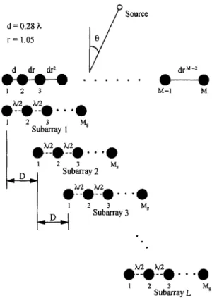
’In the first example, the array employed was a nonuniform linear array consisting of M = 24 iden- tical omnidirectional elements with the following interelement spacings:
{0.282,0.281 x 1.050.281 x 1.052,
x . . . ,0.28d x l.OP}, (21) where il is the wavelength. The above spacings were chosen so that the array had the same aperture as a 24-element ULA with an interelement spacing of :A.
d = 0.28 h r = 1.05 d dr dr2
J
Source e dr”-2 @+++ . . . a---* 12 3 M-l M I 2 Sub&ray L MSFig. 1. Geometry of real array and virtual subarrays in nonuniform linear array case.
The array was interpolated into L = 8 virtual linear subarrays, each having M, elements equally spaced by in. As depicted in Fig. 1, these subarrays were uniformly placed within the aperture of the real array. Setting the reference point at the first element of the real array, the direction vectors associated with the real array and ith virtual subarrays are given by
a(e)
[
T jy sinU,ejy(l+r)sinU ,lnd ,.(A/--11-1
= 1,e >...> eJ, (_I SI” 0
I?
hi(e) = ,j(w)N-l)sinQx [Le jx sin 0, ej2rr sin 0 >.*.>
ej(Ms-l)rrsinO T
1 ’
(22)
where d = 0.281,, r = 1.05, and the angle variable 8 is measured with respect to the broadside of the array.
T-S. Lee, T-T. Lin/Signal Processing 57 (1997) 177-194 183
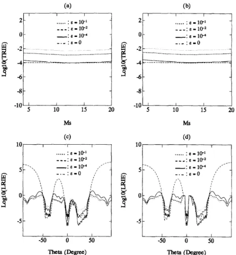
The primary and auxiliary interpolation regions were chosen as
0 = [-3”,3”] u [-45”,-35’1 U [20”,40”] , (23) with On = [-3”, 3”] and
0‘4 = [-90”, -45”] u [-35”, -lo”]
u [lo”, 20°] u [40”, 907. (24) Firstly, Figs. 2(a) and (b) show the TRIE value for the regular and SD interpolators, respectively, as a func- tion of M,, with E as a variable parameter. The TRIE is observed to be stable with respect to M,, and increase
(4
-50 0 50
Theta (Degree)
with E. This coincides with our observation regard- ing the weighting effect of E on the interpolation per- formance. Next, Figs. 2(c) and (d) show the LRIE as a function of 8 with A4, = 12, and E as a variable
parameter. Comparing the interpolation error within the primary and auxiliary regions gives an indication as to how the trade-off of interpolation performance between the two regions is achieved with a suitable E.
The interpolator with E = 0 exhibits excessively large
errors over @A, which is incurred with the ill-condition problem. In this case, E = 10e4 gives an interpolation error on the order of 10P4, and should be an ade- quate choice for the scenario considered [9]. In fact, we found that selecting an E value less than lop4 did
not give any noticeable improvement.
W
I I I 2 .a... :e-10-l i I I I 10 15 20 MS Cd) -50 0 50 meta (Degree)Fig. 2. (a), (b): Total relative interpolation error as a function of MS, with E as a variable parameter. M = 24, L = 8. (a) Regular type; (b) SD type. (c), (d): Local relative interpolation error as a function of 8, with E as a variable parameter. M=24, MS = 12 and L=S. (c) Regular type; (d) SD type. Linear array case.
184 T.-S. Lee, T.-T. Lin/ Signal Processing 57 (1997) 177-194
subarray L subarrfly 2
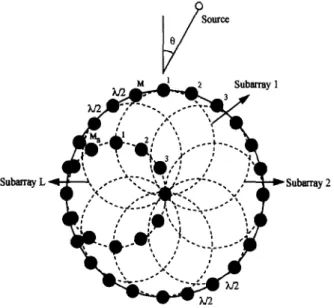
Fig. 3. Geometry of real array and virtual subarrays in the circular array case.
The example was repeated with a 24-element cir-
cular array with radius R. The elements, assumed all
identical and omnidirectional, were equally spaced
by in such that R M 1.911. The array was interpo-
lated into L = 8 virtual circular subarrays, each hav-
ing M, elements equally spaced by in. These virtual
subarrays were placed uniformly on a circle within
the aperture of the real array, as illustrated in Fig. 3.
Setting the reference point at the center of the real
array, the direction vectors associated with the real ar-
ray and ith virtual subarrays are given by
,j+%
cOS(~-~)~~,
(25)
where R, = A/(4 sin(x/M,)) is the radius of the virtual
subarrays. In this case, we assume that all the sources
are confined on the array plane such that the eleva-
tion angle is always zero, and 8 is the azimuth angle.
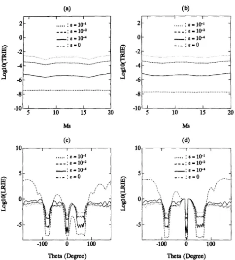
The primary and auxiliary interpolation regions were
chosen as
0 = [-5”, 5”]
U[-87.5’, -72.5’1 u [400,700], (26)
with On = [-So, 5”] and
OA = [-BOO, -87.5”] u [-72.5”, -2O”]
u [20°,400] u [70°, 180”].
(27)
Fig. 4 shows the TRIE and LRIE curves for both
types of interpolators corresponding to Fig. 2. Again
it4, = 12 was chosen for computing the LRIE. The
same trend as in the previous case is observed regard-
ing the interpolation performance with respect to E. We
note that in contrast to the linear array case, E = 0 gives
significantly better interpolation performance over 0
than other values. However, this is achieved at the
cost of excessively large errors over 0~. In this case,
E =
1O-4 gives an interpolation error on the order of
10e5, and should be a more than adequate choice for
the scenario considered.
T.-S. Lee, T.-T. Linl Signal Processing 57 (1997) 177-194 185 (4 W I 1 I I I I 2- . . . ‘s-w . 2- . . . : e - 1W .6-W ___. -__: e- 10-z O- -: e-W O- -:e-lb’ .E-O -.-. - f _._ :e- 0 -2 - -2 - ti -4 .---____________._____________________~_- ___---- $ _4 ~----______________.---__________________--- 3 c--- <a . -6 - _8 ._ _____---___. ___-_ .______---__-__ ___ -8 ---‘---“---~ -10 ; I I 1 I 10 15 20 -10 5 ’ 10 15 20 MS us (cl (4 -100 0 100 -100 0 100
Theta (Degree) meta PIP$
Fig. 4. (a), (b): Total relative interpolation error as a function of MS, with E as a variable parameter. M =24, L = 8. (a) Regular type; (b) SD type. (c), (d): Local relative interpolation __ error as a function of 8, with E as a variable parameter. M=24, MS = 12 and L= 8. (c) Regular type; (d) SD type. Circular array case.
4. Construction of optimum beamformer
This section describes the procedure for construct-
ing the beamformer with interpolated subarrays. The
procedure involves two stages:
1. Obtain the optimum subarray weight vector based
on spatially smoothed virtual subarray correlation
matrix.
2. Convert the optimum subarray weight vector back
into a full aperture weight vector for the real array.
4.1.
Stage I. Optimum subarray beamformerIf the interpolator works well, the real array will be
mapped into L nearly identical virtual subarrays. On
these subarrays we observe the transformed SD data
according to Eqs. (1) and (9):
fi=jiXFZBiis+z?l,
i=l,...,
L,where
(28)
Bi=[6i(e,),6i(e,),...,Si(e,)],
i= l,...,L, (29)ands”=[st,Sz,...,
~1~. These data are called the SD
data because they contain essentially no desired signal.
Since the virtual subarrays are identical except for a
spatial displacement, they are related through
186 T-S. Lee, T.-T. Lin/ Signal Processing 57 (1997) 177-194
where & is associated with a ‘reference’ subarray (i.e., & = & if the ith subarray is chosen as the reference),
and
,&(fk)
L _I
(31) with &(0) being the phase shift between the ith and reference subarrays induced by a wavefront from di- rection 0.
The optimum subarray beamforming weight vector, denoted as w,, is determined via the LCMV problem described in (5):
min WFfiW, w,
subject to wFb,(&) = 1, (32) where b,( (3) is the direction vector associated with the reference subarray, and d is the A4, x MS spatially smoothed virtual subarray correlation matrix given ac- cording to Eqs. (6), (28) and (30) by
i=l i=l
=
B,I?,,~ +
rs;
Q,
(33)where d,, =E{G*} is the SD source correlation ma- trix, and and Q&i; i= I (34) (35) represent the effective SD source correlation matrix and noise correlation matrix, respectively, observed
on the spatially smoothed virtual subarray. It is the averaging operation in Eq. (34) that destroys the co- herence among the interferers. Problem (32), which is similar in structure to (5), has the solution
ws = &‘b,(&), (36) where ys is a normalizing scalar.
4.2. Stage 2. Dimension recovery for full array
weight vector
As long as the condition of degree of freedom is satisfied, the resulting ‘master’ subarray beamformer constructed with w, will produce a unit gain at 0s and a deep null in each of the K interference directions such that
w;b,(8k)x0, k=l,..., K. (37)
We refer to this virtual beamformer as the ‘interference cancellation’ (IC) beamformer. If the regular type in- terpolation is adequately performed in (8), we have
k=O,l,..., K, i=l,..., L, (38) such that
(~H%)H@O) x ejti~(&)w;b,(~O) =,j&(&),
(I;Hws)Ha(&) x ej~@)w~bS(&) x 0,
k=O,l,..., K, i=l,..., L. (39) This says that the set of weight vectors
w, = ejbl(‘O) qH ws, i = 1, . . . , L, (40) acting on the real array will produce a unit gain at 80 and nulls in each of the interference directions. In other words, the look direction gain and interference nulls has been translated to wi, i = 1,. . , L, on the real array. The reason for using 4’s here instead of E’s is thus evident since z cannot retain the look direction gain of ws. The ‘back transformation’ in (40) is similar in principle to the copying of weights from the master beamformer to the slave beamformer as described in Ref. [ 111. However, a distinctive feature in Eq. (40)
T.-S. Lee, T.-T LinlSignal Processing 57 (1997) 177-194 187
is that multiple slave beamforming weight vectors are available.
The full array weight vectors wi,
i = I,.
. . ,L, can be regarded as a set of ‘basis’ vectors for the con- struction of the real array weight vector. A question now arises as to how theL
basis vectors should be combined into a single weight vector. The problem may be described as finding anL x
1 combining coefficient vector g = [gi, 92,. . . , gLIT such that the combined weight vectorL
w=
c
giWj= Wg (41)i=l
exhibits a certain optimality, where
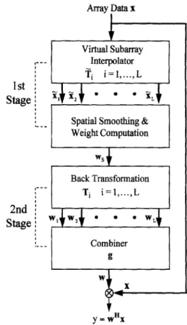
W=[w,,w2 )...) WL]. (42) The block diagram illustrating the synthesis and oper- ation of the beamformer is given in Fig. 5. Note that it is the combined weight vector w that acts on the real array data x to produce to beamformer output y. The following sections describe two types of combiners. 4.2.1.
Maximum output SNR (MSNR)
combiner
If the basis weight vectors cancel the inter- ference well, then the output due to the com- bined weight vector will contain essentially the desired signal and noise only. This is because that any linear combination of Wi,
i = 1,.
.,L,
will also cancel the interference. A reasonable cri- terion for choosing g in this case would be to maximize the output SNR of the resulting full array beamformer. This leads to the following problem:
~{l&l12)
gH@~(~d)~(~li)wg
=-g-
gHwHWg . (43) With the unknown t& replaced by the look direc- tion 60, we obtain the following equivalent prob- lem: m$ng”WHWg
subject to g”WHa(&) =
1, (44) Array Data x Virtual Subarray InterpolatorSpatial Smoothing & Weight Computation
Back Transformation
I___
1
Corn? /Fig. 5. Block diagram of two-stage interpolated beamformer.
which is again an LCMV problem whose solution is given by
g= Ys( wH w)-’ WHQo),
where again ys is a normalizing scalar.
(45)
It is interesting to note that the full array weight vector obtained by substituting Eq. (45) into (41), w = yy W( WH w-1 WHa(&), (46) can be interpreted algebraically as the orthogonal pro- jection of a(&) onto the range space of
W.
This makes sense since a(&) is the optimum weight vector which maximizes the beamformer output SNR under the quiescent (spatially white noise only) condition. On the other hand, the range space ofW
represents the ‘subspace of interference cancellation’. Projecting a(&) orthogonally onto the range space ofW
is tan- tamount to finding a vector lying in the subspace of188 T.-S. Lee, T.-T. Lb/Signal Processing 57 (1997) 177-194
interference cancellation which is closest to the opti-
mum quiescent weight vector.
The inversion of WH W in (45) dictates that W
cannot be ill-conditioned in order to avoid numerical
problems. Making W well-conditioned is equivalent
to making the vectors wi,
i =1,.
. . ,L,well separated.
This implies from (40) that the transformation matri-
ces 4,
i=1,.
. ., L,should be well separated as well.
Since these matrices are directly related to the vir-
tual subarray configuration, it is conceived that a set
of spatially well separated virtual subarrays will give
the desired W. This is another reason for restricting
the subarray number
Lin addition to that mentioned
earlier in Section 3.1.
4.2.2.
Eigen-based combinerThe MSNR combiner inherently assumes that 80
is accurate enough so that the real array pattern
w(0) will exhibit a mainlobe pointed at the desired
source. In the presence of a large pointing error,
however, it cannot guarantee a satisfactory recep-
tion of the desired signal due to the beam squint
problem. This necessitates a technique with which
the computation of weight vectors is independent
of 00. In Ref. [2], a method based on the eigen-
value decomposition (EVD) was proposed to extract
the ‘signal subspace’ from a transformed corre-
lation matrix with the interference removed. The
signal subspace is represented by an eigenvector
producing a large gain in the desired source dir-
ection. We now demonstrate that the same technique
can be readily applied to the combiner discussed
herein.
Consider the real array beamformer output as ex-
pressed by
(47)
where we have used Eq. (6) and the fact that the inter-
ference has been eliminated by W (i.e., WHa(&) M
OL, k= l,..., K). With pointing errors present, the
beamformer response g” WHa(&) is not known. In
this case, the optimum beamformer can be determined
as one that maximizes the signal-plus-noise-to-noise
ratio (SNNR). In other words, the coefficient vector g
is determined in accordance with
(48)
By maximizing the total output power with the noise
power fixed, we have in fact forced the beamformer
to produce a large gain for the desired signal. Let ui,
i=l,...
, L,be the generalized eigenvectors (GEV’s)
satisfying
WH R,x WUi = ti WH WUi,
i =1,
. . . , L,(49)
where 5,>(23
... > tL, are the corresponding gen-
eralized eigenvalues (Gev’s) arranged in descending
order. The solution to (48) is given by g = ~1, the GEV
associated with the largest Gev. By choosing w to be
W==YgWW, (50)
the beamformer will automatically produce a mainlobe
peak near
ed.
It
should be mentioned that the efficacy of the eigen-
based combiner lies in that the interference has been
suppressed sufficiently by the virtual subarray beam-
former constructed with ws, and that the transforma-
tion has successfully translated the interference nulls
from w, to each of Wi’s. Otherwise, any residual inter-
fering power left in WHRxx W will be likely stronger
than the desired signal power and thus cause conf&
sion in maximizing the SNNR by the leading GEV.
5.
Simulation results
Computer simulations were conducted to ascertain
the performance of the proposed two-stage interpo-
lated beamformer. Specifically, the performance of
the beamformer was examined against spatially white
noise, pointing errors and deviations of interpolation
region. For all cases, we assumed that the data cor-
relation matrices involved in computing the optimum
weight vectors were available, and did not concern
ourselves with the problem of estimating them.
5.1. Part 1. Linear array case
In this case, the 24-element linear array and the as-
sociated subarray configuration as described in Section
T.-S. Lee, T-T. Lin/ Signal Processing 57 (1997) 177-194 189 3.5 were employed. For all cases, the real array was
interpolated into L = 8 uniform linear virtual subarrays of size MS = 12. The desired source was at & = O”, and K = 3 interferers were generated at (31 = - 40”, e2 = 28” and e3 = 33”. The source correlation matrix was set to be 11 0 0 01 R= ss I 0 0 1000 0 100 0 100 0 0 0 100 100 I ’ (51)
which means that the second and third interferers are coherent with the same power corresponding to a signal-to-interference ratio (SIR) of -20 dB, and the first interferer is uncorrelated with the other three sources with an SIR of -30 dB. As an evaluation index, we define the beamformer output SINR as SINRO =
wdWWd2
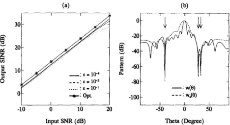
3 kc R,,(i+ 1, k+ i)WHU(ei)aH(ek)W+a~WHW i=lk=l (52) The first set of examples evaluates the performance of the interpolated beamformer against white noise. In this case, the correct look direction 00 = 0” was used (no pointing error). The primary and auxiliary interpolation regions were the same as those given in Eqs. (23) and (24), respectively. Fig. 6(a) shows the. curves of SINb versus input SNR for different values of E obtained with the MSNR type of combiner. For comparison, we also include the maximum possible output SINR (A4 times the input SNR) obtained with the optimum quiescent beamformer. We find that the beamformer performs better as E decreases, and the trend is the same for all input SNR values. This is consistent with the result that a small E leads to a small interpolation error. The SIN& values obtained with E = 1O-4 are close to the optimum ones, indicating that the second stage combiner was effective in boosting up the output SNR. It is noteworthy that the beamformer remains reliable with an SNR as low as -10 dB. This confirms that the drop in beamforming gain dueto the interpolation error is negligible as compared to the signal/interference level. As a demonstration, we show in Fig. 6(b) the beam pattern w(e) obtained with SNR = 10 dB and E = 10-4. The corresponding sub- array pattern w,(e) is also included for comparison. We observe that three deep nulls are located in the interference directions for both w(e) and w,(e), indicating that these nulls were successfully gene- rated by the subarray beamformer and then translated to the full array beamformer. It is noteworthy that the second and third interferers are separated by approximately half the 3-dB beamwidth of the subarray (% 9.6” ).
The second set of simulations examines the ef- fects of pointing errors on the proposed beamformer. In this case, the look direction 0s was varied from -5” to 5”, corresponding to a maximum pointing error of 5” (the 3-dB beamwidth of the array is ap- proximately 4.8”). The input SNR was fixed at 10 dB, and the other parameters were the same as in the previous simulation. Figs. 7(a) and (b) show the curves of SINb versus 00 for different values of a. Both types of combiners were tested for comparison. The results indicate that desired signal cancellation did not occur with pointing errors (no performance breakdown). The MSNR combiner exhibits a certain degradation in performance due to the beam squint effect. The eigen-based combiner, on the other hand, is surprisingly robust. These are confirmed by the beam patterns shown in Figs. 7(c) and (d) obtained with 8s = - 5” and E = 10P4. Clearly, both combiners successfully cancelled the three interferers even with a large pointing error. Moreover, the eigen-based combiner was able to ‘resteer’ the beam back to the desired source direction to compensate for the point- ing error at the first stage. This did not happen with the MSNR combiner.
The final set of simulations examines the effects of deviations of the interpolation region. In this case, the primary interpolation region was modified into
0 = [-3”, 3”] u [-45” + ae, -35” +Ae]
u [20”, 40”], (53)
with -10” <A0 d lo”, and @A was modified accord- ingly. This corresponds to a maximum deviation of
190 T.-S. Lee, T.-T Lin/ Signal Processing 57 (1997) 177-194
(4
0’)
I IA
I I I I 30 0 ,,/’ iii‘ -20 s E 20 is E-40 rn 5 ii -60 ,a 10 !_;;*;ii & 0” -:E-10-4 ___: E- lo-2 0 10 Input SNR (dB) -50 0 50 Theta (Dw-)Fig. 6. (a) Comparison of beamfonner output SINR versus input SNR with E as a parameter. (b) Beam patterns obtained with input SNR=lOdB and .z=IO-~. 0d=O”, Ql= -40°, &=28’ and f&=33’. &=O”. Linear array case.
04
30 I 25,; v _ * * * _ y _ * -, ---___ -:&-1V’ ___: E - lVZ . . . : e - 10-l +: opt. I 0 Theta-0 (Degree) -:a-IV4 5- ___:s- lo-2 O- . . . : e - 10’ -c: opt. / 5 -5-5 0 5 Theta-0 (Degree)(4
-20 ZT s -40 G z -60 & -80 -100 -50 0 50 -50 0 50Theta (Degree) Theta (Degree)
Fig. 7. (a), (b): Comparison of beamfonner output SINR versus pointing error with E as a parameter. (a) MSNR combiner; (b) eigen-based combiner. (c), (d): Beam patterns obtained with fIa= - So and a= 10e4. (c) MSNR combiner; (d) eigen-based combiner. Od=O’, 81 = - 40°, 82 =28’ and 83 =33’. Input SNR= 10 dB. Linear array case.
T.-S. Lee, T-7: Lin / Signal Processing 57 (1997) 177-194 191
Delta Theta (Degree)
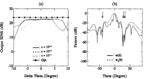
Fig. 8. (a) Comparison of beamformer output SINR versus deviation of one interpolation region with E as a parameter. (b) Beam patterns obtained with A0= - 10’ and ~=10-~. Od=O”, BI= -40°, &=28’ and 63=33’. &=O”. Input SNR =lO dB. Linear array case.
0)
Input SNR (dB) -rhea (WW
Fig. 9. (a) Comparison of beamformer output SINR versus input SNR with E as a parameter. (b) Beam patterns obtained with input SNR =lOdB andE=10V4. Od=O’, &= -80°, t$=52’ andt$=60°. &=O”. Circulararraycase.
10’ in choosing the interpolation region associated with the first interferer. Again the input SNR was fixed at IOdE& and the other parameters were the same as in the first simulation. Fig. 8(a) plots the resulting SIN& curves versus A0 for different values of E obtained with the &ENR combiner. The beamformer is ob- served to perform reasonably well for - 5’ < A 0 < 5’. Outside that region its performance is not reliable but still acceptable even when the interpolator fails to operate for the first interferer (for [A01 > 5”). This is an indication of the ‘extrapolation’ capability of the interpolator. To gain more insights, we show in
Fig. 8(b) the beam patterns obtained with A6= - 10” and E = 1 Oe4. We note that although the first interferer was not perfectly cancelled, the beamformer was still able to impose sufficient attenuation on it to prevent performance breakdown. On the other hand, the other two interferers were eliminated as desired without be- ing affected by the large deviation angle.
5.2. Part 2. Circular array case
In this subsection, we repeat the three sets of simu- lation work in Part 1 with the 24-element circular array
192 T.-S. Lee, T.-T Lin/ Signal Processing 57 (1997) 177-194
Theta-0 (Degree)
(4
Theta-0 (Degree)
(4
Theta (Degree) Theta (Degree)
Fig. 10. (a), (b): Comparison of beamfonner output SINR versus pointing error with E as a parameter. (a) MSNR combiner; (b) eigen-based combiner. (c), (d): Beam patterns obtained with 00= - 10’ and E= 10e4. (c) MSNR combiner; (d) eigen-based combiner. &=O’, 01= - SO”, 02 = 52” and 03 =60”. Input SNR= 10 dB. Circular array case.
described in Section 3.5. For all cases, the real array was interpolated into L = 8 virtual circular subarrays of IV, = 12 elements with the configuration depicted in Fig. 3. The desired source was at & = 0”) and K = 3 interferers were generated at or= - 80”) 82 = 52” and 0s =60”. The source correlation matrix was the same as (51).
The first set of examples evaluates the performance of the interpolated beamformer against white noise. Again, the correct look direction 80 = 0” was used, and the primary and auxiliary interpolation regions were the same as those given in Eqs. (26) and (27), respec- tively. Fig. 9(a) shows the curves of SINb versus in- put SNR obtained with the MSNR type combiner. The
results follow the same trend as observed in the linear array case, except that the disparity in performance as- sociated with different E values is more significant than that observed in Fig. 6(a). Also, the SINRQ values are not as close to the optimum ones as in the linear ar- ray case. We have tried smaller E but found no notice- able improvement. Choosing a larger A4, will slightly increase the output SINR, but the price is a rise in complexity. A careful examination on the two-stage behaviors of the beamformer reveals that, although the subarray beamformer successfully cancelled the interference, the second stage combiner was not able to recover the full SNR gain capability of the real array. This is deemed as the cost of imposing the
T.-S. Lee, T.-T. Linl Signal Processing 57 (1997) 177-194 193
-I--:
opt.
-10 , I I
-10 0 10
Delta Theta (Degree) Theta (Degree)
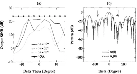
Fig. 11. (a) Comparison of beamformer output SINR versus deviation of one interpolation region with E as a parameter. (b) Beam patterns obtained with A@= - 15’ and E= 10e4. Bd=O’, Bl= - 80°, 82 =.52’ and 03 =60”. Oo=O”. Input SNR = 10 dB. Circular array case.
two-stage scheme on the circular array. The beam pat- tern obtained with SNR = 10 dB and E = 1 0P4 is given in Fig. 9(b) along with the corresponding subarray pattern. Three deep nulls are found in the interference directions for both w(0) and w,(e), as in the linear array case.
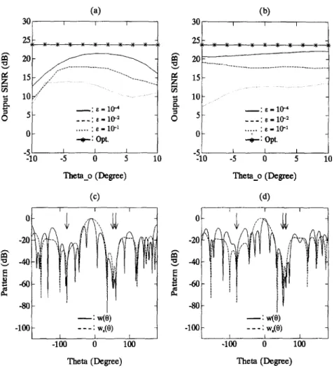
The second set of simulations examines the effects of pointing errors. The look direction 8s was varied from - 10’ to lo”, corresponding to a maximum point- ing error of 10”. The input SNR was fixed at 10 dB, and the other parameters were the same as in the pre- vious simulation. Figs. 10(a) and (b) show the curves of SIN& versus 8s for different values of E obtained with both types of combiners. The results are simi- lar in trend to those observed in Figs. 7(a) and (b). Again, the disparity among the curves is more signi- ficant than in the linear array case. Figs. 10(c) and (d) show the corresponding beam patterns obtained with 0s = - 10” and E = 10w4. The results are quite similar in nature to those observed in Figs. 7(c) and (d).
The final set of simulations examines the effects of deviations of the interpolation region. In this case, the primary interpolation region was modified into 0 = [-5”, 5”] u [-87.5’ + A& -72.5 + Ae]
u [40”, 70”], (54)
with - 15” < A 8 < 15”, and 0~ was modified accord- ingly. This corresponds to a maximum deviation of
15” in choosing the interpolation region associated with the first interferer. The input SNR was fixed at
10 dB, and the other parameters were the same as in the first simulation. Fig. 1 l(a) shows the resulting SIN& curves versus A0 for different values of E obtained with the MSNR combiner. We see that the beamformer performs well with a= lop4 as long as the interfer- ence direction is contained in the interpolation region (for IA01 ~7.5”). F or other E values, the beamformer was not as reliable in the presence of deviations. Fi- nally the beam patterns obtained with A0 = - 15” and
E = 1 Oe4 confirm that the interpolator does indeed ex- hibit a certain extrapolation effect outside its operation region. The first interferer (SIR = - 30 dB) received a gain of approximately -30 dB, resulting in an output SINR close to 0 dB.
6.
Conclusions
A method of adaptive beamforming in the pres- ence of multiple coherent interferers was presented which can be applied to arbitrary array geometry. The beamformer was developed based on interpolation, spatial smoothing and dimension recovery. The inter- polator transformed the real array into several identi- cal virtual subarrays with the desired signal removed. A spatially smoothed virtual subarray was then formed with the interferers decorrelated, on which the
194 T.-S. Lee, T-T. Lin/Signal Processing 57 (1997) 177-194
optimum subarray beamformer was constructed. By a
judiciously
designed procedure, we successfully
converted the subarray beamformer back into a full
aperture beamformer for the original array. The full
array beamformer preserves the interference nulls of
the subarray beamformer and optimizes the output
signal-noise condition. In particular, two types of
combiners were suggested for dimension recovery:
the maximum SNR combiner and the eigen-based
combiner. We showed that the eigen-based com-
biner gave better performance if the interferers were
sufficiently suppressed in the subarray beamformer.
Numerical examples confirmed that the output SINR
performance of the proposed two-stage beamformer
is quite reliable as long as the interpolation error
is confined to a moderate size. For the linear array
case, the proposed beamformer can perform almost
as well as the optimum beamformer working under
the quiescent situation.
Acknowledgements
This work was supported by the National Science
Council of R.O.C. under Grant NSC 85-2213-E-009-
017.
References
[l] B. Friedlander, “The root-MUSIC algorithm for direction finding with interpolated arrays”, Signal Processing, Vol. 30, No.1, January 1993, pp. 15-29.
[2] J.W. Kim and C.K. Un, “An adaptive array robust to beam pointing error”, IEEE Trans. Signal Process., Vol. 40, No. 6, January 1991, pp. 76-84.
[3] C.C. Ko, “Robust algorithm for combating look direction error problems”, IEEE Trans. Aerosp. Electron. Syst., Vol. 31, No. 3, July 1995, pp. 1043-1052.
[4] J.H. Lee and J.F. Wu, “Adaptive beamforming without signal cancellation in the presence of coherent jammers”, IEE Proc- F, Vol. 136, No. 4, August 1989, pp. 169-173.
[5] A.K. Luthra, “A solution to adaptive nulling problem with a look-direction constraint in the presence of coherent jammers”, IEEE Trans. Antennas Propagat., Vol. 34, No. 5,
May 1986, pp. 702-710.
[6] R.A. Monzingo and T.W. Miller, Introduction to Adaptive Arrays, Wiley, New York, NY, 1980, Chapter I, pp. 3-21.
[7] SC. Pei, C.C. Yeh and SC. Chiu, “Modified spatial smoothing for coherent jammer suppression without signal cancellation”, IEEE Trans. Acoust. Speech Signal Process.,
Vol. 36, No. 3, March 1988, pp. 412-414.
[8] T.J. Shan and T. Kailath, “Adaptive beamforming for coherent signals and interference”, IEEE Trans. Acoust. Speech Signal Process., Vol. 33, No. 6, June 1985, pp. 527-536.
[9] B.D. Van Veen and K.M. Buckly, “Beamfonning: A versatile approach to spatial filtering”, IEEE ASSP Msg., April 1988,
pp. 4-24.
[lo] A.J. Weiss and B. Friedlander, “Performance analysis of spatial smoothing with interpolated arrays”, IEEE Trans.
Signal Process., Vol. 41, No. 5, May 1993, pp. 1881-1892.
[ll] B. Widrow, K.M. Duvall, R.P. Gooch and W.C. Newman, “Signal cancellation phenomena in adaptive antennas: Causes and cures”, IEEE Trans. Antennas Propagat., Vol. 30, No. 5,
May 1982, pp. 469-478.
[12] C.C. Yeh and W.D Wang, “Coherent interference suppression by an antenna array of arbitrary geometry”, IEEE Trans. Antennas Propagat., Vol. 37, No. 10, October 1989, pp.