Lowest Landau level approximation in strongly type-II superconductors

(1)

Lowest Landau level approximation in strongly type-II superconductors

Dingping Li*

National Center for Theoretical Sciences, P.O. Box 2-131, Hsinchu, Taiwan, Republic of China Baruch Rosenstein†

National Center for Theoretical Sciences and Electrophysics Department, National Chiao Tung University, Hsinchu 30050, Taiwan, Republic of China

共Received 19 January 1999; revised manuscript received 21 April 1999兲

Higher than the lowest Landau level,共LLL兲 contributions to magnetization and specific heat of supercon-ductors are calculated using the Ginzburg-Landau equation approach. Corrections to the excitation spectrum around the solution of these equations 共treated perturbatively兲 are found. Due to symmetries of the problem leading to numerous cancellations the range of validity of the LLL approximation in the mean field is much wider then a naive range and extends all the way down to H⫽Hc2(T)/13. Moreover, the contribution of higher Landau levels共HLL兲 is significantly smaller compared to LLL than expected naively. Like the LLL part, the lattice excitation spectrum at small quasimomenta is softer than that of the usual acoustic phonons. This enhances the effect of fluctuations. The mean-field calculation extends to third order, while the fluctuation contribution due to HLL is to one loop. This complements the earlier calculation of the LLL part to two-loop order.关S0163-1829共99兲03834-5兴

I. INTRODUCTION

The Ginzburg-Landau共GL兲 effective description of high-Tc superconductors has been remarkably successful in de-scribing various thermodynamical and transport properties.1 However, when fluctuations are of importance, even this ef-fective description becomes very complicated. Some progress can be achieved when certain additional assump-tions are made. One often made additional assumption is that only the lowest Landau level共LLL兲 significantly contributes to physical quantities of interest.2–8There is a debate, how-ever, on how restrictive the LLL approximation actually is. Naively when H⬍Hc2(T)/3共see the dotted line in Fig. 1兲, even within the mean-field approximation, one should con-sider higher Landau levels共HLL’s兲 mixing in the Abrikosov vortex lattice solution of the GL equations. When fluctua-tions are included one can argue using Hartree approximation9 that the LLL range of validity is even smaller. However, direct application of the LLL scaling to magnetization and specific heat on Y-Ba-Cu-O suggest that the range of applicability is much wider—all the way down to 1⫺3T.10,7,11 It is not clear why HLL do not contribute.

In this paper we explicitly calculate the effects of HLL at low temperatures in the vortex solid or liquid phase and es-tablish the realistic range where the LLL approximation is valid共see the heavy dashed line in Fig. 1兲. We reanalyze the HLL corrections to mean-field equations going to higher or-der than in Ref. 12 and find that the expansion converges for Hc2⬎H⬎Hc2/13. Importantly, within this radius of conver-gence the LLL contribution constitutes more than 95%. Then we calculate the HLL fluctuation effects to one-loop order complementing the LLL calculation to two loops by one of us8共later referred to as I兲.

Ginzburg parameter Gi characterizing the importance of thermal fluctuations is much larger in high-Tc superconduct-ors then in the low-temperature ones. Moreover, in the

pres-ence of the magnetic field the importance of fluctuations in high-Tc superconductors is further enhanced. Under these circumstances corrections to various physical quantities like magnetization or specific heat are not negligible even at low temperatures. It is quite straightforward to systematically

ac-FIG. 1. The range of the validity of the expansions in ahand the loop expansion. The region above the dotted line is the naively expected validity range of the LLL approximation. The region above the long dashed line is the actual validity range for the ex-pansion of the mean-field equations. The loop exex-pansion applicabil-ity range lies below the dashed curves. We plot two curves with different values of Ginzburg number Gi, Gi⫽0.1, and Gi⫽0.01. The validity combining the mean-field expansion and the loop ex-pansion lies therefore between the long dashed line and the dashed curves.

PRB 60

(2)

count for the fluctuations effect on magnetization, specific heat or conductivity perturbatively above the mean-field transition line using the Ginzburg-Landau description.13 However, in the interesting region below this line it turned out to be extremely difficult to develop a quantitative theory. Within LLL in order to approach the region below the mean-field transition line T⬍Tmf(H), Thouless2 proposed a perturbative approach around the homogeneous共liquid兲 state was in which all the ‘‘bubble’’ diagrams are resumed. The series provide accurate results at high temperatures, but for the LLL dimensionless temperature aT

⬅(2Hc2

2 _/GiT

cT2H2)1/3关T⫺Tmf(H)/␲兴ⱗ⫺2 become inap-plicable. Generally attempts to extend the theory to lower temperature by Pade´ extrapolation were not successful.4 Al-ternatively, a more direct approach to low-temperature fluc-tuations physics is to start from the mean field solution and then take into account perturbative fluctuation around this inhomogeneous solution. Experimentally it is reasonable since, for example, specific heat at low temperatures is a smooth function and the fluctuation contribution experimen-tally is quite small. For some time this was in disagreement with theoretical expectations.

Eilenberger calculated the spectrum of harmonic excita-tions of the triangular vortex lattice关see Eq. 共30兲 below兴3and noted that the gapless mode is softer then the usual Gold-stone mode expected as a result of the spontaneous breaking of translational invariance. The inverse propagator for the ‘‘phase’’ excitations behaves as k_z2⫹const(k_x2⫹k_y2)2. The in-fluence of this unexpected additional ‘‘softness’’ apparently goes beyond the enhancement of the contribution of fluctua-tions at leading order. It leads to disastrous infrared diver-gences at higher orders rendering the perturbation theory around the vortex state doubtful. One, therefore, tends to think that nonperturbative effects are so important that such a perturbation theory should be abandoned.14However, it was shown in I that a closer look at the diagrams reveals that in fact one encounters actually only logarithmic divergences. This makes the divergences similar to so-called ‘‘spurious’’ divergences in the theory of critical phenomena with broken continuous symmetry and they exactly cancel out each other, provided we are calculating a symmetric quantity. Qualita-tively physics of a fluctuating D⫽3 GL model in a magnetic field turns out to be similar to that of spin systems in D⫽2 possessing a continuous symmetry. In particular, although within perturbation theory in the thermodynamic limit the ordered phase 共solid兲 exists only at T⫽0, at low tempera-tures liquid differs very little in most aspects from solid. One can effectively use properly modified perturbation theory to quantitatively study various properties of the vortex-liquid phase. This perturbative approach agrees very well with the direct Monte Carlo simulation of Ref. 7. The question arises whether one can extend the well-controlled perturbative cal-culation beyond the LLL. Sometimes a hope is expressed that the additional softness is an accidental artifact of LLL approximation. We will show that this is not so and it is a fundamental general phenomenon共see also Ref. 15兲.

The paper is organized as follows. The model is described and a perturbative mean-field solution is developed in Sec. II. The expansion parameter will be the distance from the mean-field critical line a_h⬅1

2(1⫺T/Tc⫺H/Hc2). The range of validity of the expansion and of the LLL approximation is

discussed. Then in Sec. III we derive the spectrum of exci-tations to leading order and to the next to leading order in ah. The free energy to one loop is calculated in Sec. IV. Section V contains expressions for magnetization and spe-cific heat and a discussion of the validity range of the fluc-tuation contributions calculation. Finally, we summarize the results in Sec. VI. Details of the mean-field calculation can be found in Appendix A, while details of the HLL spectrum calculation can be found in Appendix B.

II. MODEL AND THE PERTURBATIVE MEAN-FIELD SOLUTION

A. Model

Our starting point is the GL free energy:

F⫽

冕

d3x ប 2 2mab

冏

冉

ⵜ ជ_⫺ie* បcAជ

冊

␺

冏

2 ⫹ ប 2 2mc兩⳵z␺兩 2_⫹a兩_␺_兩2 ⫹b

⬘

2 兩␺兩 4_. _共1兲

Here Aជ⫽(By,0) describes a nonfluctuating constant mag-netic field. For strongly type-II superconductors (␬⬃100) far from Hc1 共this is the range of interest in this paper兲 the magnetic field is homogeneous to a high degree due to su-perposition from many vortices. For simplicity we assume a⫽␣(1⫺t)Tc, t⬅T/Tc, although this dependence can be easily modified to better describe the experimental coherence length.

Throughout most of the paper will use the following units. The unit of length is␰⫽

冑

ប2/(2mab␣Tc) and the unit of the magnetic field is Hc2, so that the dimensionless magnetic field is b⬅B/H_c2. The dimensionless Boltzmann factor in these units is 关the order parameter field is rescaled as ␺2

→(2␣T_c/b

⬘

)␺2兴: F T⫽ 1 ␻

冕

d3x 1 2兩D␺兩 2_⫹1 2兩⳵z␺兩 2_⫺1⫺t 2 兩␺兩 2_⫹1 2兩␺兩 4_. 共2兲

The dimensionless coefficient is

␻⫽

冑

2Gi␲2t, 共3兲 where the Ginzburg number is defined by Gi

⬅1 2(32␲e

2_␬2_␰_T

c␥1/2/c2h2)2 and ␥⬅mc/mab is an anisot-ropy parameter. This coefficient determines the strength of fluctuations, but is irrelevant as far as mean-field solutions are concerned.

B. Mean-field solution by expansion in ah

Now we turn to a perturbative solution of the Ginzburg-Landau equations near the mixed-state–normal-phase transi-tion line. This has been done before12to second order, how-ever, the range of applicability and precision of the LLL approximation at large␬ has not been fully explored. The z direction dependence of the solutions is trivial and will not be mentioned until fluctuations will be discussed. The expan-sion parameter is

(3)

ah⬅

1⫺t⫺b

2 . 共4兲

Rewriting the quadratic part in terms of operator 共‘‘Hamil-tonian’’兲 H⬅1

2(⫺D

2_{⫺b) whose spectrum starts from zero,}

one obtains the following free-energy density over T F T⬅ f ␻⫽ 1 ␻

冕

d2x

冉

␺*H␺⫺ah兩␺兩2⫹ 1 2兩␺兩 4

冊

_. _共5兲

The equation of motion is therefore

H␺⫺ah␺⫹␺兩␺兩2⫽0. 共6兲 This equation is solved perturbatively in ah by assuming

2

冎

, 共8兲

where a/

⬁

g_in␸n. 共10兲

Inserting into Eq.共6兲, one obtains to order a_h3:

H⌽1⫽g0␸⫺g0兩g0兩

2_␸_兩_␸_兩2_. _共11兲

Taking the inner product with␸ one finds that g0⫽

1

冑

␤A

, 共12兲

where the Abrikosov’s constant is the following average over the primitive cell:␤⫽␤A⬅

具

兩␸兩4

典

⬇1.16. Inner product with␸n determines g₁n:

g1,n⫽⫺ ␤

n

nb␤3/2, 共13兲

where␤n⬅

具

兩␸兩2␸n␸*

典

. To find g1 we need in addition also

the order a_h5/2equation:

H⌽2⫽⌽1⫺共g0兲2共2⌽1兩␸兩2⫹⌽1*␸2兲. 共14兲

The inner product with ␸ gives g1⫽3

2 n

兺

⫽1

⬁ _共_␤n_兲2

nb␤5/2. 共15兲

C. Mean-field result for free energy: Orders ah

2

and ah

3

The mean-field expression for the free energy to order a_h2 is well known. Inserting the next correction Eq.共7兲 into Eq.

共5兲 one obtains the free-energy density:

Fmf T ⫽ 1 ␻

冋

⫺ a_h2 2␤⫺ a_h3 ␤3_b _n

兺

_⫽1 ⬁ _共_␤n_兲2 n

册

⫽_␻1

冋

⫺0.43ah 2_⫺0.0078ah 3 b

册

. 共16兲

It is interesting to note that ␤n⫽0 only when n⫽6 j, where j is an integer. This is due to the hexagonal symmetry of the vortex lattice.12For n⫽6 j it decreases very fast with j: ␤6⫽⫺0.2787,␤12⫽0.0249. Because of this the coeffi-cient of the next-to-leading order is very small 共additional factor of 6 in the denominator兲. We might preliminarily con-clude therefore that the perturbation theory in ah works much better than might be naively anticipated 共see dashed line on Fig. 1兲 and can be used very far from transition line. If we demand that the correction is smaller then the main contribution, the corresponding line on the phase diagram will be b⫽0.015⫻(1⫺t). For example, the LLL melting line corresponds to ah⬃1. This overly optimistic conclusion is, however, incorrect as the calculation of the following term in Appendix A shows.

⬅

具

␸*i1␸*i2␸j1␸j2

典

and gj i when i⫽0 is defined to be equal to gj,␸i⫽␸ when i⫽0.

We already can see that g₂n and g2are proportional to g1

n

and in addition there is a factor of 1/n. Since, due to hexago-nal lattice symmetry all the g₁n, n⫽6 j vanish, so do g2n. We

(4)

checked that there is no more small parameters, so we con-clude that the leading-order coefficient is much larger than the first共factor 6⫻5), but the second is only 6 times larger than the third.

The correction to free energy is

Fmf T ⫽ 1 ␻• 0.056 62 a_h4 b2. 共19兲

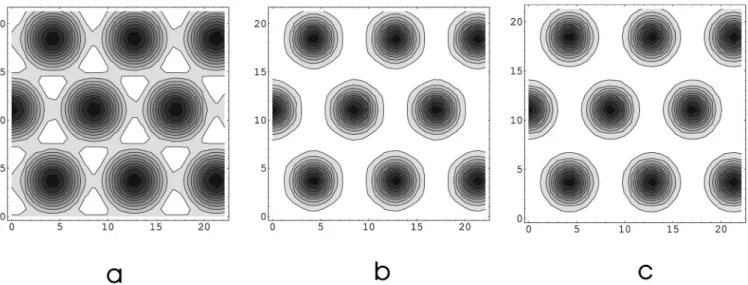
Accidental smallness by a factor of 1/6 of the coefficients in the ah/b expansion due to symmetry means that the range of validity of this expansion is roughly ah⬍6b or H⬍Hc2/13. Moreover, additional smallness of all the HLL corrections compared to the LLL means that they constitute just several percent of the correct result inside the region of applicability. To illustrate this point we plot in Fig. 2 the perturbatively calculated solution for b⫽0.1,t⫽0.5. One can see that al-though the leading LLL function has very thick vortices关Fig. 2共a兲兴, the first nonzero correction makes them of the order of the coherence length关Fig. 2共b兲兴. Following the correction of the order (a_h/b)2_{makes it practically indistinguishable from}

the numerical solution. Amazingly the order parameter be-tween the vortices approaches its vacuum value. Paradoxi-cally starting from the region close to H_c2 the perturbation theory knows to correct the order parameter so that it looks very similar to the London approximation 共valid only close to Hc1) result of well-separated vortices.

We conclude, therefore, that the expansion in ah/b works in the mean field better than one can naively expect. In the next section we investigate whether the same is true for the fluctuation contribution.

III. FLUCTUATIONS SPECTRUM A. Fluctuations to leading order in a

To find an excitation spectrum in the harmonic approxi-mation one expands the free-energy functional around the solution found in the previous section. Within the LLL ap-proximation this has been done in Ref. 3. We generalize it to the case of all the Landau levels when perturbations due to

nonlinear term are included. The fluctuating order-parameter field␺ should be divided into a nonfluctuating共mean field兲 part and a small fluctuation

␺共x兲⫽⌽共x兲⫹␹共x兲. 共20兲

The energy Eq. 共5兲 is then expanded in ␹ retaining only quadratic terms

f2⬅

冕

d2x

冋

␹*H␹⫺ah兩␹兩2⫹2兩⌽兩2兩␹兩2

⫹1

2共⌽*

2_␹2_⫹⌽2_␹*2_兲

册

_. _共21兲

Field ␹ can be expanded in a basis of quasimomentum kជ eigenfunctions: ␸kជ n ⫽

冕

kជ.n

兺

_⫽0 ⬁ ␸kជ* n 共x兲共O⫺kn ⫺iA⫺kn 兲.

FIG. 2. The density兩␺2_{兩 of the mean-field Abrikosov solution for b⫽0.1,t⫽0.5. 共a兲 is the lowest order approximation 共LLL兲. 共b兲 is the} solution with the next-order correction included, while in共c兲 the next-next-order correction is included.

(5)

In terms of these fields representing ‘‘optical’’ and ‘‘acous-tic’’ phonons Eq.共21兲 takes a form

f2⫽

冕

kជ.n

兺

_⫽1 ⬁ 共nh⫺ah兲共Ok n O_⫺kn ⫹A_knA_⫺kn 兲

⫺ah共OkO⫺k⫹AkA⫺k兲共24兲

⫹

兺

i, j⫽0 ⬁ A_kiA_⫺kj K_ki, j⫹O_kiA_⫺kj L_ki, j ⫹O_⫺ki A_kjM_ki, j⫹O_kiO_⫺kj N_ki, j where elements of the matrix are

.

. We will use definitions

.

When an index is zero we drop it throughout the paper. For example, when n⫽0, we refer to ␤_kn as ␤k, and when k

⫽0,␤k

n_⫽_␤n_{, etc.}_兲.

Considering to order ah above matrix element i, j⫽0 of

K,L, M ,N is K1⫽2 ␤ ␤k⫺ 1 ␤Re␥k, N1⫽ 2 ␤ ␤k⫹ 1 ␤Re␥k 共29兲 L₁⫽M_k⫽⫺1 ␤Im␥k.

In deriving this we have used a property ␤k⫽␤⫺k.

We now diagonalize the matrix to find the eigenstates of LLL 共which is of order ah兲. Eigenvalues are

⑀A⫽ah

冉

⫺1⫹ 2 ␤ ␤k⫺

1

(6)

⑀O⫽ah

冉

⫺1⫹ 2 ␤ ␤k⫹

1 ␤兩␥k兩

冊

,

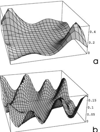
as was found originally by Eilenberger.3 The ‘‘acoustic’’ branch is shown in Fig. 3共a兲. The rotation transforming in to these eigenstates is A ˜ k⫽cos ␪k 2 Ak⫹sin ␪k 2 Ok, 共31兲 O˜k⫽⫺sin ␪k 2 Ak⫹cos ␪k 2 Ok,

where ␥_k⬅兩␥_k兩exp关i␪_k兴. A similar calculation for the nth Landau level gives the spectrum

␧A,O n _⫽a h

冉

⫺1⫹ 2 ␤

具

兩␸兩2␸k* n ␸k n

_典

_⫿1 ␤兩

具

共␸*兲2␸k n ␸⫺kn

典

兩

冊

. 共32兲

B. Spectrum of fluctuations beyond leading order in ah

In this subsection we calculate the correction of eigenval-ues of LLL to order a_h2. The Hamiltonian Hˆ in addition has the ah part Hˆ1given in Eq.共27兲 also has the ah

2

part Hˆ2. As

will be explained in the next section, we will need only the correction to the LLL to the ah

⫺ 6 ␤ ␤n 2 Im␥k⫹ 4 ␤ ␤nIm¯␥k n

册

.

Note that we do not show L2 and M2separately as our result

will depend only on L2⫹M₂. According to the degenerate perturbation theory we need to diagonalize Hˆ1which already

has been done in the previous subsection and then use the resulting states A˜kand O˜k to calculate the second-order cor-rection to the eigenvalue:␧_k(2)⫽a_h2(Ediag⫹Eoffdiag). The diag-onal contribution is

Ediag⬅

具

A˜k兩Hˆ2兩A˜k

典

⫽

冉

cos ␪k 2

冊

2 K2⫹N2

冉

sin␪k 2

冊

2 ⫹共L2⫹M2兲sin ␪k 2cos ␪k 2 . 共34兲

Substituting the matrix elements Eq. 共33兲 we obtain Ediag⫽

兺

n⫽1 ␤n nb␤2

再

3␤n ␤ 共2␤k⫺兩␥k兩兲⫺2关Re␤k n ¯ ⫹Re¯␤_⫺kn ⫺cos␪kRe␥k n ¯ ⫺sin␪kIm␥k n ¯ 兴

冎

. 共35兲

In the off-diagonal contribution

TABLE I. Contributions to the free energy of mixing the LLL with HLL. Given in units of 12␴bah 3/2

.

Level n 1 2 3 4 5 6 7 8

A mode ⫺0.253 ⫺0.082 ⫺0.053 ⫺0.063 ⫺0.063 0.247 ⫺0.017 ⫺0.005

O mode ⫺0.230 ⫺0.086 ⫺0.051 ⫺0.023 ⫺0.012 0.018 ⫺0.003 ⫺0.001

. 共36兲 Details of the calculation of these matrix elements can be found in Appendix B together with definitions of quantities F. The result is Eoffdiag⫽⫺1 b

兺

n 1 n

再

1 ␤2[兩Fk n_共1兲兩2_⫹兩F ⫺k n _共1兲兩2_⫹兩F k n_共2兲兩2_⫹兩F ⫺k n _共2兲兩]2_⫹cos␪k ␤2 关兩Fk n_共1兲兩2_⫹兩F ⫺k n _共1兲兩2_⫺兩F k n_共2兲兩2 ⫺兩F_⫺kn _共2兲兩2_兴⫹2 sin␪k ␤2 Im 关F⫺k n _共1兲F ⫺k *n_共2兲⫺F k *n_共1兲F k n_共2兲兴

冎

_. _共37兲

A similar result for Okcan be obtained by changing the sign of cos␪kand the sign of sin␪kin the formula above.

It is crucial to see whether there is a k2 term in higher orders for the acoustic branch A. We calculated numerically the contributions to the spectrum until n⫽8. All the k2 con-tributions to any of them cancel, as it was proved in Ref. 15. Moreover even all the k4 contributions for odd n cancel al-though the even n give a negative contribution to the rota-tionally symmetric combination (k_x2⫹k_y2)2. Numerically the coefficients are 2.2⫻10⫺6, 5.0⫻10⫺5, ⫺6.3⫻10⫺6, 4.7

⫻10⫺7_{for n}_{⫽2,4,6,8 correspondingly. The resulting}

correc-tion to the spectrum of the acoustic branch due to the n⫽2 level is shown in Fig. 3共b兲.

After we have established the spectrum of the elementary excitations of the Abrikosov lattice, we are ready to calculate the fluctuation contributions to various physical quantities.

IV. FLUCTUATION CONTRIBUTIONS TO FREE ENERGY, MAGNETIZATION AND SPECIFIC HEAT

Higher Landau levels contribution to free energy The thermal fluctuation part is

⫺T ln关Z兴⬅Fmf⫹Ffluc; Ffluc⫽T₂

兺

n⫽0 ⬁

再

Tr ln

冋

␧_An共k兲⫹kz 2 2

册

⫹Tr ln

冋

␧O n_共k兲⫹kz 2 2

册

冎

共38兲 ⫽TLx 2_L z␴b

兺

n⫽0 ⬁ 关

具

冑

␧A n_共k兲

_典

_⫹

_具

冑

_␧ O n_共k兲

_典

_兴,

where ␴⬅1/

冑

22␲ and we performed the integration over kz.

The LLL contribution to order

冑

ah in two dimensions

共2D兲 has been calculated by Eilenberger.3_{The 3D result for}

the density of the free energy is8

Ffluc (1/2) T ⫽␴bah 1/2_关

_具

冑

_␧ A (1)_共k兲

_典

_⫹

_具

冑

_␧ O (1)_共k兲

_典

_兴⫽3.16_␴ bah 1/2 . 共39兲

We calculated its higher ah correction which is of order ah

3/2

using Eqs.共35兲 and 共37兲

Ffluc (3/2) T ⫽ 1 2␴bah 3/2

冋

冓

␧A (2)_共k兲

冑

␧A (1) 共k兲

冔

⫹

冓

␧O (2)_共k兲

冑

␧O (1) 共k兲

冔

册

⫽⫺0.445␴ba_h3/2. 共40兲 As noted below␧A (2) (k) and␧A (2)

(k) given in the last section contain contributions from mixing with all the HLL’s. Table I details contributions to this term from levels until n⫽8. The contributions are negative for all n⫽6 j where j is an integer and positive otherwise.

The contribution of HLL is Ffluc T ⫽␴bn

兺

⫽1 ⬁ 关

具

冑

nb⫹ah␧A n_共k兲

_典

_⫹

_␧ O n_共k兲

_典

_兴⫹O共a h 2_兲 ⫽_T1共Ffluc(0)_⫹Ffluc(1)_兲. _共41兲

(8)

The first divergent共as powers 3/2 and 1/2 in the ultraviolet兲 term renormalizes energy. However, it has a finite magnetic-field-dependent part which should be calculated by subtract-ing the b⫽0 value of the free energy. The proper regulariza-tion is made by restricting the number of Landau levels and then showing that after regularization the answer does not depend on it. The calculation is the same as the one done in the normal phase 共obviously uv divergences are insensitive to the phase in which they are calculated兲, see for details and discussion, Ref. 16. The result is

Ffluc (0)

T ⫽0.526␴b

3/2_. _共42兲

This exhibits the diamagnetic nature of the bosonic field.17 The second term is proportional to兺1/

冑

n and also diverges but only as power 1/2 in the ultraviolet and renormalizes ah. To see this we calculate the sum

具

␧A n_{共k兲⫹␧} O n_共k兲

_典

k⫽⫺2⫹ 4 ␤

具具

兩␸兩2␸k* n_␸ k n

_典

x

典

k⫽⫺2⫹ 4 ␤. 共43兲

The last equality follows from the curious property of ␸k*

⫹␻␴ 2_b2_a h ⫺1_关c ⫺1 (1)_兴,

where the coefficients共upper index is the power of␻and the lower index is the power of a_h) are

c₂(⫺1)⫽⫺0.434, c₃(⫺1)⫽⫺0.0078, c0(0)⫽0.526,

共46兲

c_1/2(0)⫽316, c₁(0)⫽1.06, c3/2(0)⫽⫺0.445, c_⫺1(1)⫽0.118, and ␻ is defined in Eq.共3兲. The last term is the two-loop contribution calculated in I. One clearly see that ␻bah⫺3/2 always appears together with an important ‘‘loop factor’’␴

⫽ 1/23/2_␲_{⯝0.11. The expansion parameter therefore is}

␴␻ba_h⫺3/2⫽␲

冑

2Gi tb

共1⫺t⫺b兲3/2⫽

1

冑

2␲兩aT兩3/2 .

In the last equation aTis the often used dimensionless LLL temperature introduced by Thouless.2For Gi⫽0.01 the con-dition␴␻ah⫺3/2⬍1 is represented by the area above the dot-ted line in Fig. 1.

Correspondingly the scaled magnetization is m

Now we address the question whether the GL energy it-self can be reliably used in the region of applicability stated above. The GL free energy is an effective energy obtained after integrating out microscopic degrees of freedom ␸micr 共for example, quantum electron fields in the BCS or Hubbard

model兲. Formally one writes exp兵⫺␤FGL关␺兴其⫽

冕

␸micr

␦„␺⫺␺共␸micr兲…exp兵⫺␤F关␸micr兴其,

共49兲

where the functional F关␸micr兴 describes a microscopic theory

共one has to make also the quantum-mechanical average not

shown explicitly兲. The order-parameter field is a function of the microscopic field 共bilinear in electron field in BCS兲. Without detailed knowledge of the microscopic theory the functional FGL关␺兴 could be quite general, however near T_c for H⫽0 or more generally near Hc2(T) the order parameter is small and one can expand on it. Gorkov derived the coef-ficients of the GL theory from BCS.13While some such deri-vations of the GL theory exist for high-Tcmaterials,

18

also in the magnetic field,19 here we show the consistency of the approach within the area of applicability of the approxima-tion we use. Of course, in particular microscopic theories the range of applicability might be larger. Generally the require-ments are the following. Terms 兩␺兩6,兩␺兩8, . . . should be small compared to 兩␺兩4 _{in the GL free energy Eq.} _{共1兲. In}

addition gradients should be small so that higher共covariant兲 derivatives can be neglected compared to兩D␺兩2.

Our perturbative solution ␺⬀

冑

a_h, therefore, 兩␺兩6_⬀a

h

3

while 兩␺兩6⬀a_h2. Therefore, in the leading order兩␺兩6 can be neglected. In higher orders, those higher terms do contribute. In the next leading term兩␺兩6 should be phenomenologically included, while 兩␺兩8 not and so forth. As far as higher de-rivatives are concerned we have shown that even for HLL

兩D␺兩2_⬀ba

h and thus higher derivative terms appear only at quite high order. Therefore, we can take the GL free energy, Eq. 共1兲, as the free energy of the system to leading order. Thus in the LLL regime defined here in the paper, the GL theory shall describe the physics correctly. Higher-order cor-rections require more free parameters.

VI. CONCLUSION

In this paper we showed why the LLL results are often valid far beyond the naive limit of applicability of the ap-proximation for both the mean-field and the fluctuation parts. Our results are valid strictly speaking between the long-dashed line representing H⫽Hc2(T)/13 and one of the dashed curves indicating the range of validity of the loop expansion for the fluctuation contribution共depends on value of the Ginzburg number Gi). For nonfluctuating strongly type-II superconductors our results can be directly checked by experiments done at low temperature or numerical solu-tion共or even the ‘‘London limit approximation’’兲 and are in clear agreement. For small, but not very small Ginzburg pa-rameter Gi one can compare with existing Monte Carlo

共MC兲 simulations7,20_{or experiments. Of course, one can use}

the existing high-temperature expansion2to interpolate to the present expansion range. Results for LLL were presented in I and the HLL do not alter them significantly. The agreement

with the MC simulations is very good although obviously the melting transition is not seen. As argued in I it is not ex-pected to exist within the present model. The HLL do not change this conclusion. That the ‘‘supersoft’’ A mode has a propagator 1/关k_z2⫹const(k_x2⫹k_y2)2兴 beyond the LLL approxi-mation lays to rest a suspicion that this is a fluke due to LLL.15This indicates that this unusual ‘‘softness’’ is due to some underlying symmetry which has yet to be explicitly identified.

ACKNOWLEDGMENTS

We are grateful to our colleagues A. Knigavko, B. Bako, V. Yang. B.R. is grateful to G. Kotliar, A. Balatsky, L. Bu-laevskii, Y. Kluger, and R. Sasik for numerous discussions in Los Alamos where this work started. We also thank R. Ikeda for bringing Ref. 15 to our attention. The work is part of the NCTS topical program on vortices in high-Tc and was sup-ported by the NSC of Taiwan.

APPENDIX A: THIRD-ORDER CORRECTION TO THE MEAN-FIELD SOLUTION AND FREE ENERGY

In this appendix we provide some details of the third or-der correction in the a_hcalculation of the mean-field solution of the GL equations.

To calculate g₂n, one takes the inner product of␸n on the two sides of Eq. 共14兲 and obtains Eq. 共17兲. To calculate g2, we need to consider the GL equation to order a_h7/2:

H⌽3⫽⌽2⫺关共⌽0兲2_⌽2_*_⫹共⌽_1兲2_⌽0_*_{⫹2兩⌽0兩}2_⌽2

⫹2兩⌽1兩2_⌽0_*_兴. _共A1兲

n_⫽0

冋

nbg₁ng₂n⫺1 2共g1 n_兲2

册

Ok n_兩Hˆ1兩O k

典

⫽ 1 ␤

冋

␤⫺k*n⫹␤k n_⫹1 2共␥⫺k* n_⫹_␥ k n_兲

册

具

Ak兩Hˆ1兩Ok n

_典具

O_kn兩Hˆ1兩Ok

典

⫹c.c. ⫽ 2 ␤2关Fk* n_共1兲F k n_共2兲⫺F ⫺k n _共1兲F ⫺k *n_{共2兲兴⫹c.c.,} where Fk n_共1兲⫽_␤ k n_⫺1 2␥k n , 共B5兲 F_kn共2兲⫽␤_kn⫹1 2␥k n_.

Finally, we can show that

Eoffdiag⫽⫺1 b

兺

n 1 n

再

1 ␤2关兩Fk n 共1兲兩2_⫹兩F ⫺k n 共1兲兩2_⫹兩F k n 共2兲兩2 ⫹兩F_⫺kn _共2兲兩2_兴⫹cos␪k ␤2 关兩Fk n_共1兲兩2_⫹兩F ⫺k n _共1兲兩2 ⫺兩Fk n_共2兲兩2_⫺兩F ⫺k n _共2兲兩2_兴 ⫹sin␪k ␤2 2 Im关F⫺k n _共1兲F ⫺k *n_共2兲⫺F k *n_共1兲F k n_共2兲兴

冎

. 共B6兲

*Electronic address: [email protected] †_{Electronic address: [email protected]}

1_{G. Blatter, M. V. Feigel’man, V. B. Geshkenbein, A. I. Larkin,} and V. M. Vinokur, Rev. Mod. Phys. 66, 1125共1994兲. 2_{D. J. Thouless, Phys. Rev. Lett. 34, 946}_{共1975兲; G. I. Ruggeri and}

D. J. Thouless, J. Phys. F 6, 2063共1976兲; S. Hikami, A. Fujita, and A. I. Larkin, Phys. Rev. B 44, 10 400共1991兲.

3_{G. Eilenberger, Phys. Rev. 164, 628} _{共1967兲; K. Maki and H.} Takayama, Prog. Theor. Phys. 46, 1651共1971兲.

4_{G. J. Ruggeri, J. Phys. F 9, 1861}_{共1979兲; M. A. Moore, Phys. Rev.} B 41, 7124共1996兲.

5_{M. A. Moore, Phys. Rev. B 39, 136}_{共1989兲; 45, 7336 共1992兲; 55,} 14 136共1997兲.

6_{Z. Tesanovic et al., Phys. Rev. Lett. 69, 3563} _{共1992兲; Z.} Te-sanovic and A. V. Andreev, Phys. Rev. B 49, 4064共1994兲. 7_{R. Sasik and D. Stroud, Phys. Rev. Lett. 75, 2582}_共1995兲. 8_{B. Rosenstein, Phys. Rev. B 60, 4268}_共1999兲.

9_{I. D. Lawrie, Phys. Rev. B 50, 9456}_共1994兲.

10_{B. Zhou et al., Phys. Rev. B 47, 11 631}_{共1993兲; S. W. Pierson} et al., Phys. Rev. Lett. 74, 1887共1995兲; Phys. Rev. B 53, 8638

共1996兲.

11_{S. W. Pierson, O. T. Valls, Z. Tesanovic, and M. A. Lindemann,} Phys. Rev. B 57, 8622共1998兲.

12_{G. Lascher, Phys. Rev. 140, A523}_共1965兲.

13_{M. Tinkham, Introduction to Superconductivity} _{共McGraw-Hill,} New York, 1996兲.

14_{G. J. Ruggeri, Phys. Rev. B 20, 3626}_共1978兲.

15_{A. Ikeda, T. Ohmi, and T. Tsuneto, J. Phys. Soc. Jpn. 59, 1740}

共1990兲; 61, 254 共1992兲; A. Ikeda, ibid. 64, 1683 共1994兲; 64,

3925共1995兲.

16_{D. Jana, Nucl. Phys. B 473, 659}_{共1996兲; 485, 747 共1997兲.} 17_{B. Simon, Phys. Rev. Lett. 36, 1083} _{共1976兲; S. Sinha and J.}

Samuel, Phys. Rev. B 50, 13 871共1994兲.

18_{Y. Ren, J. H. Xu, and C. S. Ting, Phys. Rev. Lett. 74, 3680}

共1995兲; P. I. Soininen, C. Kallin, and A. J. Berlinsky, Phys. Rev.

B 50, 13 883共1994兲; A. J. Berlinsky et al., Phys. Rev. Lett. 75, 2200共1995兲.

19_{M. Rasolt and X. Tesanovic, Rev. Mod. Phys. 64, 3}_共1992兲. 20_{X. Hu, S. Miyashita, and M. Tachiki, Phys. Rev. B 58, 3438}