On: 24 April 2014, At: 21:18 Publisher: Taylor & Francis
Informa Ltd Registered in England and Wales Registered Number: 1072954 Registered office: Mortimer House, 37-41 Mortimer Street, London W1T 3JH, UK
Journal of the Chinese Institute of Engineers
Publication details, including instructions for authors and subscription information: http://www.tandfonline.com/loi/tcie20
A multi
‐stage IIR time domain equalizer for OFDM
systems with ISI
Wen‐Rong Wu a & Chun‐Fang Lee b
a
Department of Communication Engineering , National Chiao Tung University , Hsinchu, 30010, Taiwan, R.O.C.
b
Department of Communication Engineering , National Chiao Tung University , Hsinchu, 30010, Taiwan, R.O.C. Phone: 886–3–5731647 Fax: 886–3–5731647 E-mail:
Published online: 04 Mar 2011.
To cite this article: Wen‐Rong Wu & Chun‐Fang Lee (2010) A multi‐stage IIR time domain equalizer for OFDM systems with ISI, Journal of the Chinese Institute of Engineers, 33:3, 475-487, DOI: 10.1080/02533839.2010.9671635
To link to this article: http://dx.doi.org/10.1080/02533839.2010.9671635
PLEASE SCROLL DOWN FOR ARTICLE
Taylor & Francis makes every effort to ensure the accuracy of all the information (the “Content”) contained in the publications on our platform. However, Taylor & Francis, our agents, and our licensors make no
representations or warranties whatsoever as to the accuracy, completeness, or suitability for any purpose of the Content. Any opinions and views expressed in this publication are the opinions and views of the authors, and are not the views of or endorsed by Taylor & Francis. The accuracy of the Content should not be relied upon and should be independently verified with primary sources of information. Taylor and Francis shall not be liable for any losses, actions, claims, proceedings, demands, costs, expenses, damages, and other liabilities whatsoever or howsoever caused arising directly or indirectly in connection with, in relation to or arising out of the use of the Content.
This article may be used for research, teaching, and private study purposes. Any substantial or systematic reproduction, redistribution, reselling, loan, sub-licensing, systematic supply, or distribution in any
form to anyone is expressly forbidden. Terms & Conditions of access and use can be found at http:// www.tandfonline.com/page/terms-and-conditions
A MULTI-STAGE IIR TIME DOMAIN EQUALIZER FOR OFDM
SYSTEMS WITH ISI
Wen-Rong Wu and Chun-Fang Lee*
ABSTRACT
In an orthogonal frequency division multiplexing (OFDM) system, it is known that when the delay spread of the channel is larger than the cyclic prefix (CP) size, intersymbol interference will occur. The time-domain equalizer (TEQ), designed to shorten the channel impulse response (CIR), is a common device to solve this problem. Conventionally, the TEQ is treated as a finite-impulse-response (FIR) filter, and many TEQ design methods have been proposed. However, a wireless channel typically has multi-path responses, exhibiting FIR characteristics. Thus, the corresponding TEQ will have an infinite impulse response (IIR), and the FIR modeling of the TEQ is inefficient, i.e., the required order for the TEQ will be high. The conventional ap-proach will then suffer from the high computation complexity problem, both in the derivation of TEQ and in the operation of channel shortening. In this paper, we pro-pose a new scheme to overcome these problems. In the derivation of the TEQ, we propose to use a multistage structure, replacing a high-order TEQ with a cascade of several low-order TEQs. In the shortening operation, we propose to use an IIR TEQ approximating a high-order FIR TEQ. Since the ideal TEQ exhibits low-order IIR characteristics, the order of the IIR TEQ can be much lower than the FIR TEQ. Simu-lations show that while the proposed method can reduce computational complexity significantly, its performance is almost as good as existing methods.
Key Words: orthogonal frequency division multiplexing, time domain equalizer, infinite impulse response, steiglitz-McBride method.
*Corresponding author. (Tel: 886-3-5731647; Fax: 886-3-5710116; Email: wrwu@faculty.nctu.edu.tw; jefflee.cm89g@nctu.edu.tw)
The authors are with the Department of Communication Engineering, National Chiao Tung University, Hsinchu 30010, Taiwan, R.O.C.
I. INTRODUCTION
Orthogonal frequency division multiplexing (OFDM) is a multicarrier transmission technique popu-larly used in wireless systems, such as IEEE 802.11g, DAB, DVB, etc. The OFDM divides the available signal band into many subchannels and allows a subcarrier to be used in each subchannel for data transmission. In general, a cyclic prefix (CP) is added in front of an OFDM symbol to avoid intersymbol interference (ISI). The CP length is at least equal to or greater than the length of the channel impulse response (CIR). Since the CP will reduce the transmission efficiency, a large-size CP is not desirable. Thus, the choice of the CP size is often a compromise between the tolerated
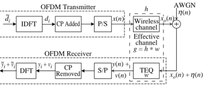
length of the CIR, and the data throughput. As a result, in some scenarios the length of the CIR will exceed the CP range. When this happens, ISI is induced and the system performance is degraded. A simple rem-edy for this problem is to apply a time domain equal-izer (TEQ) such that the CIR can be shortened into the CP range. Fig. 1 shows a typical OFDM system, with a TEQ added for the purpose of channel shortening. TEQ development originated from the commu-nity of wireline communications (e.g. ADSL). The modulation scheme in wireline applications is called discrete multi-tone (DMT). DMT is essentially the same as OFDM. The main difference lies in the fact that the DMT performs bit-loading while the OFDM does not. With bit-loading, the transmission can ap-proach the maximum channel capacity. Many algo-rithms have been proposed for the design of a TEQ in a DMT system (Chow and Cioffi, 1992; Melsa et al., 1996; Al-Dhahir and Cioffi, 1996; Arslan et al., 2001; Van Acker et al., 2001; Henkel, et al., 2002;
Vanbleu et al., 2004; Martin et al., 2005; Kim and Powers, 2005; Wu and Lee, 2005). Recently, some methods have been extended to OFDM systems (Zhang and Ser, 2002; Leus and Moonen, 2003; Yang and Kang, 2006; Lee and Wu, 2007; Wu and Lee, 2007; Rawal, et al., 2007; Rawal and Vijaykumar, 2008). For a DMT system, a TEQ design minimizing the mean-squared-error (MMSE) was first developed by Chow and Cioffi (1992). The MMSE method allows an adap-tive structure and its computational complexity is low. Treating the TEQ design as a pure channel shorten-ing problem, Melsa et al. (1996) proposed a criterion to maximize the shortened signal-to-noise ratio (SSNR), defined as the ratio of the energy of the TEQ shortened response inside and outside the CP range. This method is then referred to as the maximized SSNR (MSSNR) method. The work proposed by Al-Dhahir and Cioffi (1996) first considers capacity maximiza-tion in TEQ design. With a geometric SNR (GSNR) maximization, a constrained nonlinear optimization problem was obtained. Taking both residual ISI and channel noise into account, a method referred to as maximum bit rate (MBR) (Arslan et al., 2001; Vanbleu et al., 2004) was then proposed. To improve the performance, the inter-carrier interference (ICI) is taken into consideration by Henkel et al. (2002). It was found that the aforementioned methods shared a com-mon mathematical framework based on the maximi-zation of a product of generalized Rayleigh quotients (Martin, et al., 2005).
The methods mentioned above all conduct the TEQ design in the time-domain. Another approach, treating the problem in the frequency-domain, was first proposed by Acker et al. (2001) for DMT sys-tems, and later by Leus and Moonen (2003) for MIMO OFDM systems. This method, referred as per-tone equalization (PTEQ), allows an equalizer designed for the signal in each tone. Using the computational ad-vantage of the fast Fourier transform technique, TEQ filtering operations can be effectively implemented in the discrete-Fourier transform (DFT) domain. It has been shown that the PTEQ scheme can outper-form conventional TEQ schemes. However, PTEQ requires a large-size memory for storage and is
potentially higher in computational complexity (Martin, et al., 2005). Another method called sub-symbol equalization (SSE) (Kim and Powers, 2005) also designs the TEQ in the frequency domain. It uses the conventional zero-forcing frequency domain equalizer to obtain the equalized time-domain signal. The drawback of the SSE is that it is only applicable to a certain type of channels.
As mentioned, for OFDM systems, no bit-load-ing is conducted and the purpose of the TEQ is just to reduce the ISI. The bit-error-rate (BER) is then the criterion to evaluate the performance of an OFDM system. In general, the larger the SSNR, the smaller the ISI and the smaller the BER we can have. Thus, the MSSNR criterion, which cannot achieve the maxi-mum capacity in DMT systems, is adequate in OFDM systems. The MSSNR TEQ for OFDM systems has been studied by Yang and Kang (2006). With the original MSSNR method, the TEQ length must be constrained to be smaller than or equal to the CP length. In a work by Yang and Kang (2006), a modi-fied MSSNR TEQ method was proposed to solve the problem. Using this method, the limitation of the TEQ tap length can be removed. Furthermore, an adaptive TEQ method based on the least mean-square (LMS) algorithm is also proposed to track the chan-nel variation. Since the convergence of the LMS algorithm is slow, the QR-recursive least square (QR-RLS) algorithm is further proposed by Rawal and Vijaykumar (2008) for TEQ adaptation.
For all methods discussed above, the TEQ is treated as a finite-impulse-response (FIR) filter. However, a wireless channel typically has multi-path responses, exhibiting FIR characteristics. It can be shown that the ideal TEQ has infinite impulse response (IIR) characteristics, and its order is low. As a result, the FIR modeling of the TEQ is inefficient. To achieve a high SSNR, the TEQ order must be high. Conven-tional approaches then suffer from the high compu-tational complexity problem, either in the derivation of TEQ or in the operation of channel shortening.
In this paper, we propose a low-complexity scheme to overcome the problem mentioned above. The basic idea is to use an IIR TEQ instead of an FIR TEQ for the channel shortening. However, the direct derivation of an IIR TEQ from the channel response is a difficult job. In this paper, we propose to use a two-step approach. In the first step, we derive a high-order FIR TEQ. In the second step, we convert the FIR TEQ into a low-order IIR TEQ. In the deriva-tion of the FIR TEQ, we propose to use a multi-stage (MS) structure. Instead of a single-stage (SS) high-order TEQ, we propose to use a cascade of several low-order TEQs. For conventional TEQ design meth-ods such as proposed by Melsa et al. (1996) or Arslan et al., (2001), matrix operations are frequently required,
OFDM Receiver OFDM Transmitter DFT IDFT CP Added CP Removed P/S S/P TEQ w Wireless channel Effective channel g = h * w AWGN (n) di x(n) d~i yi + vi yi + vi ~ ~ h xo(n) η η xo(n) + (n) y(n) + v(n)
Fig. 1 An OFDM system with TEQ
and the computational complexity is O(N3) (Yang and Kang, 2006) where N is the TEQ order. Thus, if N is large, the required computational complexity is high. With our MS structure, the computational complex-ity for the FIR TEQ derivation can be dramatically reduced. Since the ideal TEQ exhibits low-order IIR characteristics, the order required for an IIR TEQ will be much lower than that of an FIR TEQ. To convert an FIR filter into an equivalent IIR form, we apply the Steiglitz McBride method (SMM) (Steiglitz and McBride, 1965) to do the job. Simulations show that while the proposed method can reduce the computa-tional complexity significantly, performance remains excellent. In this paper, we will mainly use the MSSNR method (Melsa et al., 1996) as our TEQ design method. It can produce good BER performance for OFDM sys-tems (Yang and Kang, 2006). Note that the idea of the IIR TEQ was first proposed in the works of Wu and Lee (2007) and Lee and Wu (2007). In Rawal et al. (2007), an IIR TEQ based on the QR-RLS adap-tive algorithm was also proposed. However, it is well-known that the stability of an adaptive IIR filter cannot be guaranteed. This is different from the SMM we use, where convergence is guaranteed (Stoica and Söderström, 1981; Cheng and Stonick, 1994; Netto et al., 1995; Regalia et al., 1997).
This paper is organized as follows. In Section II, we give the general signal model of an OFDM system. In Section III, we briefly review the IIR char-acteristics of the TEQ, derive the MS FIR TEQ, de-tail the proposed IIR TEQ scheme, and analyze its complexity. Section IV shows the simulation results. Finally, Section V draws conclusions.
II. SIGNAL MODEL
Let M be the DFT size, L the CP length, K = M + L the OFDM symbol length, I the channel length, and N the TEQ length. In addition, let n be the signal index, i the OFDM symbol index, both in the time domain, and k the subchannel index in the DFT domain, where 0 ≤ k ≤ M – 1. Let * be the linear convolution operation, and denote [.]T, and [.]H as the
transpose, and the Hermitian operation for a vector or matrix, respectively. Denote 0p as the p × 1 zero
column vector, 1p the p × 1 unity column vector, 0pxq
the p × q zero matrix, and Ip the p × p identity matrix.
A common model of an OFDM system with TEQ design is shown in Fig. 1. On the OFDM transmitter side, denote the i-th transmitted data symbol as d~i =
[ d~i(0), ...,
~
di(M – 1)]T, where
~
di(k) is the (k + 1)-th
element of d~i. Taking the M-point inverse DFT
(M-IDFT) to d~i, we can then obtain the corresponding
time domain signal, denoted as di. That is, di =
[di(0), ..., di(M – 1)]T = M1FH
~
di, where F = [ f (0),
f (1), ..., f (M –1)] is an M × M DFT matrix, f(k) = [1,
e–j2πk/M, ..., e–j2π(M – 1)k/M]T. Subsequently, appending
the CP and conducting parallel-to-serial conversion, we obtain the transmitted signal x(n). Here, n = iK + l, and
x(iK + l) = di(l + M – L) , for 0≤ l ≤ L – 1 ,
di(l – L) , for L≤ l ≤ K – 1 , (1)
where di(l) is the (l + 1)-th element of di. The signal
x(n) is then transmitted over a wireless channel with FIR and corrupted by the additive white Gaussian noise (AWGN).
Let the wireless CIR be represented as h = [h(0), ..., h(I – 1)]T, and AWGN as η(n). x(n) is
as-sumed independent of the noise η(n). Denote the noise-free channel output signal as xo(n), where
xo(n) = x(n) * h(n). At the receiver side, both xo(n)
and η(n) are first filtered by an N-tap TEQ. Let the TEQ coefficients be denoted as w = [w(0), ..., w(N – 1)]T. Also let the corresponding TEQ-filtered output
of xo(n) and that of the channel noise be y(n) and
v(n), where y(n) = xo(n) * w(n) and v(n) = η(n) *
w(n), respectively. Moreover, without loss of generality, let the synchronization delay be zero in the following paragraphs. Performing the serial-to-parallel conversion and removing the CP, we can ob-tain the i-th received signal-only OFDM symbol as yi
= [y(iK + L), ..., y((i + 1)K –1)]T. Let the
correspond-ing i-th noise symbol vector at the TEQ input and output be ηi = [η(iK + L), ..., η((i + 1)K – 1)]T and vi
= [v(iK + L), ..., v((i + 1)K –1)]T, respectively.
From Fig. 1, we can see that the transmitted sig-nal x(n) passes the wireless channel, h(n), and the TEQ, w(n). Let g(n) = h(n) * w(n) be the equivalent channel response (ECR), and g = [g(0), ..., g(J – 1)]T,
where J = I + N – 1. Assume that J < M, and we can decompose g into g = gS + gI, where gS = [g(0), ...,
g(L – 1), 0T
J – L]T is the desired shortened channel
response, and gI = [0LT, g(L), ..., g(J –1)]T the residual
ISI response.
We can then express gS and gI in terms of the
channel matrix H and the TEQ vector w as gS = DSHw
and gI = DIHw, respectively, where DS = diag[1LT,
0T J – L], DI = IJ – DS = diag[0LT, 1J – LT ], and H = h(0) 0 0 0 h(1) h(0) 0 0
h(I – 1) h(I – 2) h(I – 3) h(I – N) 0 h(I – 1) h(I – 2) h(I – N + 1)
0 0 0 h(I – 1)
J× N
.
(2)
Here, diag[.] denotes a diagonal matrix with the vec-tor inside the bracket as its diagonal elements. We can reexpress gS and gI as gS = [gS(0), ..., gS(J – 1)]T,
and gI = [gI(0), ..., gI(J – 1)]T, respectively, where
gS(l) is the (l + 1)-th element of gS, and gI(l) that of
gI. Let yS(n), yI(n) be the desired part and the
re-sidual ISI part of y(n). Thus we have y(n) = yS(n) *
yI(n), where yS(n) = x(n) * gS(n), and yI(n) = x(n) *
gI(n). Consequently, we can also decompose yi as
yi = yS, i + yI, i, (3)
where yS, i = [yS(iK + L), ..., yS((i + 1)K –1)]T, and
yI, i = [yI(iK + L), ..., yI((i + 1)K –1)]T.
III. PROPOSED IIR TEQ METHOD In this section, we first describe the IIR charac-teristics of the TEQ in Section III.1. Then we derive the MS FIR TEQ in Section III.2. Based on the result, we then derive the proposed IIR TEQ scheme in Sec-tion III.3. Finally, we analyze the computaSec-tional com-plexity of the proposed scheme in Section III.4. 1. IIR Characteristic of the TEQ
A typical wireless channel generally has multipath responses, which can be modeled as an FIR system. In this paragraph, we show that the TEQ for an FIR channel will exhibit an IIR characteristic. Recall that a wireless CIR h = [h(0), ..., h(I – 1)]T
has an FIR where the channel length exceeds the CP size, that is, I > L. Without loss of generality, we let h(0) = 1. Denote the transfer function of the channel as H(z). Then,
H(z) = 1 + h(1)z–1 + ... + h(I – 1)z–I + 1 = (1 – z1z–1)(1 – z2z–1) ... (1 – z
I – 1z–1), (4)
where z1, ..., zI – 1 are I – 1 zeros of H(z) and |z1| ≤ |z2|
... ≤ |zI – 1|. We can further express H(z) as a cascade
of three FIR channels, i.e., H(z) = H0(z)H1(z)H2(z) where H0(z) has m0 zeros all located inside the unit circle, H1(z) has m1 zeros all located on the unit circle, and H2(z) has m2 zeros all located outside the unit circle. Note that m0 + m1 + m2 = I – 1. Now, suppose we want to shorten the wireless channel into the CP range. In other words, the TEQ must shorten at least I – L channel taps. We have three cases to discuss, i.e., (i) I – L ≤ m0, (ii) m0 < I – L ≤ m0 + m2, (iii) m0 + m2 < I – L. For case (i), the TEQ can be an IIR filter having I – L poles of {z1, ..., zI – L}. Denoting the
transfer function of the TEQ as W(z), we can have
W(z) = 1
(1 – z1z– 1)(1 – z2z– 1) (1 – zI – Lz– 1)
. (5)
In this case, I – L zeros of H(z) is canceled by I – L poles of W(z), and the channel response can be perfectly shortened. For case (ii), we can let m0 ze-ros of H(z) be canceled by m0 poles of W(z) obtained from H0(z). However, there are I – L – m0 zeros can-not be canceled. Note that if we substitute for z with z–1 in H
2(z), the resultant transfer function will have its zeros located inside the unit circle. This indicates that the zeros of H2(z–1) can also be canceled by an IIR filter if the time index goes from 0 to –∞. Al-though the IIR filer is not realizable, it can be ap-proximated by an non-causal FIR filter. Thus, we have the TEQ as
W(z) = W0(z)
(1 – z1z– 1)(1 – z2z– 1) (1 – zm0z– 1)
, (6)
where W0(z) is the FIR filter designed to cancel the response of the I – L – m0 zeros. In this case, the channel can be shortened, but not perfectly. The per-formance depends on the dimension of W0(z). As is known, zeros on the unit circle cannot be canceled. Thus, for case (iii), the channel response cannot be shortened into the CP range. Since the number of the taps to be shortened is generally much smaller than the channel length itself, case (i) will be observed in most environments.
From the above discussion, we conclude that the TEQ possesses an IIR characteristic in wireless channels. Note that this property is quite different from the wireline applications where the CIR can be modeled as a low-order IIR system (Crespo and Honig, 1991). Thus, a low-order FIR TEQ can effec-tively shorten the channel. This is also the main dif-ference between the application of the TEQ in DMT and OFDM systems.
2. Derivation of MS FIR TEQ
As shown in Fig. 1, the objective of the TEQ is to shorten the CIR length I to the CP size, L. As discussed, for wireless channels, the required FIR TEQ order for the desired shortening may be long. As we will see, the derivation of the MSSNR TEQ relies on matrix operations having the computational complexity of O(N3). If N is large, the computational complex-ity will be high. Here, we propose an MS structure to alleviate this problem. We approach the original SS TEQ with a cascade of multiple TEQs. It is simple to see that the TEQ order in each stage can be made much smaller than that of the original one. Let the number of stages be V, the TEQ vector in the l-th stage be wl, and its order be Nl, that is, wl = [wl(0), ...,
wl(Nl – 1)]T, where 1 ≤ l ≤ V. In each stage, we can
derive the TEQ using the conventional MSSNR me-thod.
For each individual stage of the MS structure, let the ECR at the l-th stage be denoted as gl. Then, gl
= gl – 1 * wl, where g0 = h and 1 ≤ l ≤ V. Here, the
convolution operator ‘*’ is applied for vectors. In the l-th stage, the TEQ shortens the CIR for designated Pl
taps. In other words, after the l-th TEQ, the length of target-impulse-response becomes I – Σl
i = 1Pi. Hence,
the total target-shortening-length is ΣV
l = 1Pl = I – L
and the overall equivalent TEQ length is ΣV
l = 1Nl – V +
1. Furthermore, the overall TEQ response w is equal to the cascade of the individual TEQs, that is, w = w1 * w2 * ... wV.
As mentioned in Section II, assume that the syn-chronization delay is zero, and let gl = [gl(0), ..., gl(Jl
–1)]T, where J
l is the ECR length at the l-th stage,
and Jl = Jl – 1 + Nl – 1, 1 ≤ l ≤ V. Note that J0 = I is the
original CIR length. We can then decompose gl into
two parts, the desired shortened channel response gS, l = [gl(0), ..., gl(Ll – 1), 0TJl – Ll]T and the residual ISI gI, l = [0TLl, gl(Ll), ..., gl(Jl – 1)]T, where Ll = I –
Σl
j = 1Pl. That is, gl = gS, l + gI, l. Then, we can rewrite
gS, l and gI, l as
gS, l = DS, lHlwl,
gI, l = DI, lHlwl, (7)
where DS, l = diag[1TLl, 0TJl – Ll], DI, l = diag[0TLl, 1TJl – Ll], and Hl a Jl× Nl matrix consisting of a shift version of
the ECR gl – 1, Hl= gl – 1(0) 0 0 gl – 1(1) gl – 1(0) 0 gl – 1(Jl – 1– 1) gl – 1(Jl – 1– 2) gl – 1(Jl – 1– Nl) 0 gl – 1(Jl – 1– 1) gl – 1(Jl – 1– Nl+ 1) 0 0 gl – 1(Jl – 1– 1) Jl× Nl . (8)
The SSNR at the TEQ output of the l-th stage for the OFDM receiver is then defined as
SSNRl= gS, lH g S, l gI, lHg I, l =wl HH l HD S, l HD S, lHlwl wlHH l HD I, l HD I, lHlwl =wl HA lwl wlHB lwl , (9) where gH
S, lgS, l is the desired signal power, gHI, lgI, l
the residual ISI power, Al = HHlDHS, lDS, lHl, and Bl =
HH
lDHI, lDI, lHl.
The optimal TEQ for the MSSNR method can be obtained through the maximization of the SSNR. The rows of DI, lHl are formed by the shifted
version of the CIR and the rank of DI, lHl is Jl× Nl.
Consequently, the matrix Bl is of full rank Nl × Nl
and also positive definite. Hence, Bl can be
decom-posed by using the Cholesky decomposition, that is, Bl = BlBHl. We can define a vector yl = BHlwl, and
then wl = (BHl)–1yl. Thus, wHlBlwl = yHlyl, and wHlAlwl
= yH
l(Bl)–1Al(BHl)–1yl = yHlAlyl, where Al = (Bl)–1Al
(BH
l)–1. As a result, SSNRl = yHlAlyl/yHlyl has a form
of Raleigh quotient. It is well known that optimal yl, O maximizing the quotient SSNRl can be obtained by
choosing the eigenvector corresponding to the maxi-mum eigenvalue of Al (Chong and Zak, 2001). Thus,
the optimal TEQ vector wl, O is
wl, O = (BHl)–1yl, O (10)
and the corresponding optimal SSNRl is
SSNRl, O=wl, O H A lwl, O wl, OH B lwl, O =λl, (11) where λl is the maximum eigenvalue of Al. Different
from DMT systems, the MSSNR TEQ has been shown to have good performance in OFDM systems (Yang and Kang, 2006).
After deriving TEQ vectors {w1, O, w2, O, ..., wV, O}
for all V stages, we can have the equivalent optimal TEQ vector wO as
wO = w1, O * w2, O * ... wV, O (12)
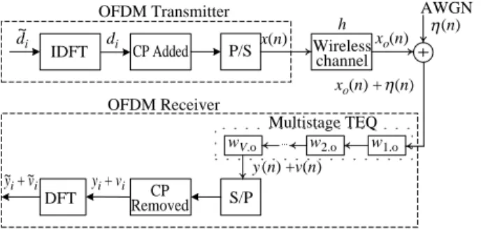
This result is also shown in Fig. 2. 3. Derivation of IIR TEQ
As shown in Section III.1, the TEQ for the wire-less channel possesses a low-order IIR property. Thus, a conventional FIR TEQ achieving satisfactory performance requires a high order. This will require heavy computations in the shortening operation. To solve the problem, we then propose to convert the
FIR TEQ obtained in Eq.(12) to an equivalent IIR TEQ. By doing so, we can effectively reduce the re-quired computational complexity for the shortening operation. Here, we use the Steiglitz-McBride method (SMM) to do the job.
The SMM is an iterative method for IIR system identification (Steiglitz and McBride, 1965). Its structure is shown in Fig. 3, in which c(n), x(n), and r(n) denote the impulse response, the input signal, and the output signal of the plant, respectively. Here, the plant is an IIR system and its transfer function can be represented as a rational function as
C(z) =A(z)B(z). (13)
Also let Cm(z) =Am(z)
Bm(z)
(14) be the estimated transfer function of the plant in the m-th iteration, where Am(z) = ΣQj = 0αj(m)z–j, Bm(z) = 1
– ΣP
j = 1βj(m)z–j. Note that Q and P are the orders of
A(z) and B(z), respectively. Assume that in the (m-1)-th iteration, optimal Bm – 1(z) and Am – 1(z) have
been obtained. To conduct the m-th iteration, the SMM first filters the plant output, r(n), and its input, x(n), with 1/Bm – 1(z). The resultant outputs, u(n) and
v(n), are then fed to Bm(z) and Am(z), respectively.
Optimal Bm(z) and Am(z) can then be obtained by
mini-mizing the average-squared-error (ASE) power of the two outputs. It is simple to see that if the algorithm converges, i.e., Bm – 1(z) = Bm(z), then the plant is
iden-tified as Am(z)/Bm(z).
Put the unknown parameters βj(m) and αj(m)
to-gether to form a vector ΘΘ (m) as Θ
Θ (m) = [β1(m), ..., βP(m), α0(m), ..., αQ(m)]T,
(15) and also define a vector ΦΦ(n) as
Φ
Φ(n) = [v(n – 1), ..., v(n – P), u(n), ...,
u(n – Q)]T. (16)
Define the error signal between the filtered out-puts of u(n) and v(n) as em(n). Then, we have
em(n) =
Σ
αj(m)v(n – j) – u(n) j = 0 Q +Σ
βj(m)u(n – j) j = 1 P =ΦΦT(n)ΘΘ(m) – u(n) . (17) If we collect the observations of u(n) and v(n) in a time window with size N′, we can then have N′ samples of the error signal which can be expressed asem(n) = Ψ (n)ΘΨ Θ (m) – u(n), (18)
where em(n) = [em(n), em(n – 1), ..., em(n – N′ + 1)]T,
u(n) = [u(n), u(n – 1), ..., u(n – N′ + 1)]T, and Ψ (n) =Ψ [ΦΦ(n), ΦΦ(n – 1), ..., ΦΦ(n – N′ + 1)]T. Thus, we can use the least-squares (LS) method to obtain the opti-mal estimate of ΘΘ (m). The criterion for the LS method is to minimize the ASE power, denoted as ξ[ΘΘ (m)], given by Steiglitz and McBride (1965),
ξ[ΘΘ (m)] = ||em(n)||2 = ||ΨΨ (n)ΘΘ (m) – u(n)||2,
(19) The solution to the LS Eq. (19) can be written as
Θ
Θ (m) = (ΨΨT(n)ΨΨ (n))–1ΨΨT(n)u(n). (20)
Then, 1/Bm(z) is used to filter r(n) and x(n), and
u(n) and v(n) is obtained for the LS solution in the next iteration. Since the SMM is an iterative al-gorithm, it requires an initial estimate of B0(z). A simple method for this problem is just to let B0(z) = 1. In this case, v(n) is the input of the plant which is x(n), and u(n) is the corresponding output, i.e., u(n) = r(n). For IIR filter design, stability is always an issue. The stability and the convergence of the SMM have been investigated. Interested readers may refer to the works by Stoica and Söderström (1981), Cheng and Stonick (1994), Netto et al. (1995), and Regalia et al. (1997).
We summarize the procedure of the proposed TEQ design method as follows. Firstly, we apply the MS structure and use the conventional MSSNR method to obtain an FIR TEQ wl, O for each stage,
where 1 ≤ l ≤ V. By cascading the multiple stages of TEQs wl, O, we can obtain the equivalent optimal TEQ
OFDM Receiver OFDM Transmitter IDFT DFT CP Added CP Removed P/S S/P Multistage TEQ Wireless channel h
wV.o w2.o w1.o
yi + vi ~ ~ y i + vi y (n) +v(n) di di ~ x(n) xo(n) η xo(n) + (n) AWGN (n) η x(n) Plant C(z) r(n) u(n) v(n) Bm – 1(z)–1 Bm(z) Bm – 1(z)–1 Am(z) em(n) + –
Fig. 2 An OFDM system with multistage TEQ
Fig. 3 System model for Steiglitz McBride method
wO in Eq. (12). Treating wO as the impulse response
of an IIR plant, we can then apply the SMM to con-vert the FIR TEQ into an equivalent IIR TEQ, efficiently.
4. Complexity Analysis
In this section, we discuss the issue of compu-tational complexity of the proposed algorithm. We first compare the design complexity of the conven-tional SS and the proposed MS FIR TEQ. For fair comparison, we let the order of the conventional SS TEQ be equal to the equivalent order of the MS TEQ. The computational complexity of the SS MSSNR TEQ method is shown to be 38N3/3 + IN2 (Yang and Kang, 2006), where N is the SS TEQ length. Thus, that of the proposed MS method is 38ΣV
l = 1N3l/3 + IΣVl = 1N2l,
where Nl is the l-th stage length of the proposed TEQ,
V the number of multi-stages, and I the length of the CIR. Hence, the MS approach can greatly reduce the required computational complexity. As an example, we let N = 16, V = 3, and I = 25. The computational complexity of the MS TEQ is only 13.8% of that of the SS TEQ. The improvement comes from the fact that the computational complexity of the MSSNR method is O(N3). As a result, when N is large, the complexity grows fast.
We now consider the computational complexity of the SMM. For simplicity, let the data window size of the SMM, denoted as N′, be equal to the FIR TEQ filter order N. It can be shown that the computational complexity of the SMM is O(m[(P + Q + 1)3 + (P + Q + 1)2N + (P + Q + 1)N]), where m is the iteration number. Although the computational complexity of the SMM has the same order as that of the MSSNR, its actual complexity will be much lower. This is due to two facts. First, as we will see in the next section, the SMM converges very fast, usually within five iterations. Second, in typical applications, P + Q is usually much smaller than N. As a result, the over-head introduced by the SMM is not significant.
We now evaluate the computational complexity during the shortening operation. Note that the short-ening operation has to be conducted for every input data sample. It solely depends on the number of taps in the TEQ. Thus, the computational complexity for the conventional FIR TEQ is O(N), while that for the proposed IIR TEQ is O(P + Q + 1). Since P + Q is usually much smaller than N, the computational com-plexity of the IIR TEQ is much smaller than the FIR TEQ. Using a typical example, the proposed algo-rithm can save approximately up to 70% of the com-putations without compromising the BER performance (Lee and Wu, 2007). When M and L are large, as found in many practical OFDM systems, the reduc-tion in computareduc-tional complexity can be very significant.
IV. SIMULATIONS
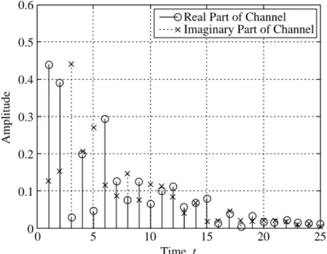
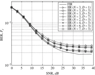
The simulation setup is described as follows. The OFDM system we use has symbol size of 64, and CP size of 16. The wireless channel is generated using an exponential-decay power profile. The channel is quasi-static and its response changes for every OFDM packet. In our simulations, we assume that the CIR is known or can be well estimated. The length of the wireless CIR is assumed to be 25, exceeding the CP size. A typical wireless CIR is shown in Fig. 4. Chan-nel noise is modeled as the AWGN, and added at the channel output. All FIR TEQs considered in the simu-lations have an order of 16. They are designed with the MSSNR method (Melsa et al., 1996), which has been shown to be a good compromise between com-plexity and BER performance (Yang and Kang, 2006). In the figures shown, N and D stand for the number of zeros and poles used in the IIR TEQ, respectively. In the first set of simulations, we evaluated the impact of the number of poles and zeros used in the IIR TEQ, and the convergence rate of the SMM. Fig. 5 shows the relationship between the ASE power and the iteration numbers, under the variation of the pole/ zero order of the IIR TEQ. We can see that as the number of poles (or zeros) increases, the error power decreases. This is not surprising since more degrees of freedom can be used to reduce the ASE power. Fig. 6 shows the relationship between the residual ISI power and the iteration numbers, under the same set-ting as that in Fig. 5. Since the residual ISI power is not the criterion to be minimized, an IIR TEQ with higher order does not necessarily yield a smaller re-sidual ISI power. Note that the rere-sidual ISI power relates to the BER, directly. Also shown in Figs. 5 and 6, we can see that the SMM converges to a stable value very quickly. The required number of itera-tions is typically below 5. We then consider the BER
0.6 0.5 0.4 0.3 0.2 0.1 0 Amplitude 0 5 10 15 Time, t 20 25 Real Part of Channel Imaginary Part of Channel
Fig. 4 A typical wireless channel impulse response
performance of the IIR TEQs discussed above, as shown in Fig. 7. The behavior of the BER perfor-mance in Fig. 7 is similar to that of the residual ISI power in Fig. 6. This is consistent with the assertion we just mentioned. Note that the choice of the order of the IIR TEQ is a compromise between the BER performance and the computational complexity. From simulations, we found that a good choice for the num-bers of zeros and poles are 3 and 3, respectively. Fig. 8 shows an example of the impulse responses of the FIR filter and its equivalent IIR filter (fitted with the SMM). Here, the number of poles is 3, that of zeros is also 3, and the iteration number used in the SMM is 5. We can see that the fitted IIR TEQ can approach the original FIR TEQ well.
The performance and the computational com-plexity of the proposed algorithm depend on the parameters it uses such as the number of stages, the filter order at each stage, and the target channel length
to be shortened (TLS) at each stage. Before the ac-tual application of the proposed algorithm, we need to determine those parameters. We then need some design guidelines in order to obtain optimal results. Since theoretical analysis is difficult, we use simula-tions to do the job here. Table 1, 2, and 3 show the different parameter settings for simulations. The sec-ond column in the tables numbers the test TEQs used in the simulations, and the third column gives the number of stages used in the MS structure. The fourth column gives the order of the TEQ used at each stage, in which the notation a, b, ... indicates that the TEQ order for the first stage is a, that for the second stage is b, and so on. The last column gives the TLS, where the notation c, d, ... indicates that the TLS for the first stage is c, that for the 2nd stage is d, and so on. The BER performance of the MSSNR (Melsa et a l. , 1 9 9 6 ) a n d t h e p r o p o s e d m e t h o d a r e t h e n evaluated. All the simulations are evaluated with
Fig. 5 Average-squared-error of IIR TEQ fitted with SMM (for various pole/zero orders)
10–1 10–2 Average-Square-Error, ASE 0 5 10 Iteration 15 20 N = 3, D = 1 N = 3, D = 3 N = 3, D = 5 N = 3, D = 7 N = 2, D = 3 N = 4, D = 3 N = 6, D = 3 N = 7, D = 3 10–1
Residual ISI Power
0 5 10 Iteration 15 20 N = 3, D = 1 N = 3, D = 3 N = 3, D = 5 N = 3, D = 7 N = 2, D = 3 N = 4, D = 3 N = 6, D = 3 N = 7, D = 3
Fig. 6 Residual ISI power of IIR TEQ fitted with SMM (for vari-ous pole/zero orders)
Fig. 7 BER performance of IIR TEQ fitted with SMM (for vari-ous pole/zero orders)
Fig. 8 Impulse response of an FIR TEQ and its fitted IIR TEQ 10–1 10–2 BER, Pe 0 5 10 15 20 SNR, dB 30 25 35 40 FIR IIR (N = 3, D = 1) IIR (N = 3, D = 3) IIR (N = 3, D = 5) IIR (N = 3, D = 7) IIR (N = 2, D = 3) IIR (N = 4, D = 3) IIR (N = 6, D = 3) IIR (N = 7, D = 3) 0.14 0.12 0.1 0.08 0.06 0.04 0.02 0 Amplitude 0 2 4 6 8 10 12 Time Index 14 16 18 FIR Impulse Response IIR Impulse Response
1000 OFDM packets, where each OFDM packet con-tains 60 OFDM symbols. We first see the effect of the number of processing stages. Table 1 shows the parameter setting for this purpose. Here, we let the equivalent order of the MS TEQ be the same in all settings. The number of stages we tried are 2, 3, 4, and 5, corresponding to TEQ #1a, #1b, #1c, and #1d, respectively. The equivalent TEQ filter order is 16 for all 4 test TEQs. The TEQ filter orders are 8, 9, 6, 6, 6, 5, 5, 5, 4, and 4, 4, 4, 4, 4, respectively. And the TLSs for the test TEQs are 4, 5, 3, 3, 3, 3, 2, 2, 2, 2, 2, 2, 2, 1, respectively. Fig. 9 shows the BER performance comparison for settings in Table 1. We can see that as the number of stages increases, although the amount of computation can be reduced, the BER performance degrades. It is apparent that the BER performance for the SS TEQ (the plot of MSSNR TEQ) is superior to that of the multistage ones. This is not surprising since the original MSSNR design is a joint optimization approach (for all tap weights), while the MS structure is not. From Fig. 9,
Table 1 Simulation scenario 1 (for various IIR orders)
Fig. # TEQ # Multistage order TEQ order per stage TLS per stage
Fig. 9 TEQ #1a 2 8, 9 4, 5
TEQ #1b 3 6, 6, 6 3, 3, 3
TEQ #1c 4 5, 5, 5, 4 3, 2, 2, 2
TEQ #1d 5 4, 4, 4, 4, 4 2, 2, 2, 2, 1
Table 2 Simulation scenario 2 (for various pole/zero orders per stage)
Fig. # TEQ # Multistage order TEQ order per stage TLS per stage
Fig. 10 TEQ #2a 2 16, 16 4, 5
TEQ #2b 2 13, 16 4, 5
TEQ #2c 2 11, 16 4, 5
TEQ #2d 2 8, 16 4, 5
TEQ #2e 2 6, 16 4, 5
TEQ #2f 2 4, 16 4, 5
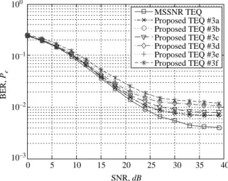
Fig. 11 TEQ #3a 2 16, 16 4, 5
TEQ #3b 2 16, 13 4, 5
TEQ #3c 2 16, 11 4, 5
TEQ #3d 2 16, 9 4, 5
TEQ #3e 2 16, 6 4, 5
TEQ #3f 2 16, 4 4, 5
Table 3 Simulation Scenario 3 (for various TLS per stage)
Fig. # TEQ # Multistage order TEQ order per stage TLS per stage
Fig. 12 TEQ #4a 2 16, 16 7, 2
TEQ #4b 2 16, 16 6, 3 TEQ #4c 2 16, 16 5, 4 TEQ #4d 2 16, 16 4, 5 TEQ #4e 2 16, 16 3, 6 TEQ #4f 2 16, 16 2, 7 10–1 10–2 10–3 100 BER, Pe 0 5 10 15 20 SNR, dB 30 25 35 40 MSSNR TEQ Proposed TEQ #1a Proposed TEQ #1b Proposed TEQ #1c Proposed TEQ #1d
Fig. 9 BER performance of experiment #1 (for various stage numbers)
we can see that it is adequate to let the number of stages be 2 or 3 (that is, TEQ #1a and #1b), a good compromise between complexity and BER per-formance.
We then evaluate the effect of the filter order used at each stage. Table 2 gives the setting for simulations. Here, the number of stages is set as 2, the highest order for each stage is set as 16, and the TLSs for the test TEQs are all fixed to 4, 5. Figs. 10 and 11 show the simulation results. From the figures, we can see that the larger the filter order, the better the BER performance we can have. However, as the filter order of one stage increases, the compu-tational complexity increases accordingly. Thus, there is a compromise between the TEQ order and the performance. Also from Fig. 11, we can see that as the filter order at the second stage decreases (that in the first stage is fixed), the performance degrades, but the degradation is not severe. In contrast, from Fig. 10, we see that as the filter order of the first stage decreases (that in the second stage is fixed), the per-formance degradation is more severe. This is because the residual ISI of the first stage will propagate to the second stage, and the TEQ in the second stage cannot compensate for that effect completely. Thus, the TEQs in early stages play more important roles than those in following stages. We should give a higher order for the TEQs in the early stages. On the other hand, the shortening work is also relatively easier at early stages, and a higher order for the TEQ may be not required. In summary, we may let the TEQ order be roughly equal for all stages. This is an important property the MS structure has.
Table 3 shows the settings of the TEQ in sce-narios with various TLSs. Here, the number of stages is still set to 2, and the TEQ tap length for both stages is set to 16. Fig. 12 shows the simulation results. We see that if the TLS of the first stage is in a smaller order, such as the case of TEQ #4d, #4e and #4f, the BER performance is generally better than that of other cases. The reason is similar to the results in Figs. 10
and 11. As the TLS of the first stage increases, the residual ISI of the first stage will become larger and it propagates to the second stage. The TEQ in the second stage cannot compensate for that effect. However, if the TLS of the first stage becomes too small, the corresponding TLS of the second stage be-comes large and the required filter order of the sec-ond stage becomes high. Then the computational complexity of the TEQ will be increased. With a larger residual ISI, no matter whether in the first or second stage, the performance of the TEQ will be degraded. Thus, it is better to distribute the required TLS to all stages, evenly. This is another important property the MS structure has.
Based on the simulation results, we can obtain some design guidelines for the MS design. Firstly, the number of stages used should not be too large, i.e., 2 or 3. Secondly, the filter order for each stage
10–1 10–2 10–3 100 BER, Pe 0 5 10 15 20 SNR, dB 30 25 35 40 MSSNR TEQ Proposed TEQ #2a Proposed TEQ #2b Proposed TEQ #2c Proposed TEQ #2d Proposed TEQ #2e Proposed TEQ #2f
Fig. 10 BER performance of experiment #2 (for various TEQ or-ders in the first stage)
10–1 10–2 10–3 100 BER, Pe 0 5 10 15 20 SNR, dB 30 25 35 40 MSSNR TEQ Proposed TEQ #3a Proposed TEQ #3b Proposed TEQ #3c Proposed TEQ #3d Proposed TEQ #3e Proposed TEQ #3f
Fig. 11 BER performance of experiment #3 (for various TEQ or-ders in the second stage)
10–1 10–2 10–3 100 BER, Pe 0 5 10 15 20 SNR, dB 30 25 35 40 MSSNR TEQ Proposed TEQ #4a Proposed TEQ #4b Proposed TEQ #4c Proposed TEQ #4d Proposed TEQ #4e Proposed TEQ #4f
Fig. 12 BER performance of experiment #4 (for various TLS per stage)
can be made roughly equal. The order is selected with a compromise between complexity and performance. For example, an appropriate filter order for a two-stage structure may be 8, 9. Thirdly, the total TLS can also be evenly distributed to all TEQs. In other words, the TLS for each stage can also be set roughly equal. Or, that in early stages is somewhat lower. For example, an appropriate TLS value for a two-stage structure can be 4, 5 or 3, 6.
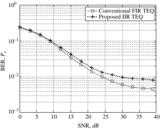
According to the above design guidelines, we can determine proper values for the parameters. It turns out that the number of stages is 2, the filter or-der per stage is 8, 9, the TLS is 4, 5. Fig. 13 shows the simulation results with the settings. As we can see, the BER performance of the proposed IIR TEQ is slightly worse than that of the original FIR TEQ. The complexity ratio of the IIR TEQ compared to that of the FIR TEQ in TEQ derivation, and in shortening, is only 33% and 37%, respectively. We can then conclude that the proposed IIR TEQ is much more efficient than the conventional FIR TEQ.
V. CONCLUSIONS
In this paper, we propose to use the IIR TEQ for channel shortening in OFDM systems. The ob-jective is to reduce the computational complexity of the conventional FIR TEQ. Since the direct deriva-tion of the IIR TEQ is difficult, we use a simpler two-step approach. In the first two-step, we use a multistage structure to obtain the FIR TEQ. In the second step, we use the SMM to convert the FIR TEQ into an equivalent IIR TEQ. Since the ideal TEQ exhibits low-order IIR characteristics, the order of the IIR TEQ can be much lower than that of the FIR TEQ. Also, the TEQ derivation with the MS structure can be much more efficient than the conventional SS structure. We
then obtain a low-complexity TEQ, both in deriva-tion and the shortening phase. Simuladeriva-tions show that while the proposed method can reduce the computa-tional complexity significantly, its performance is almost as good as that of the existing methods.
NOMENCLATURE
A(z), Am(z) zero part of C(z) and Cm(z), respectively
Bl Cholesky decomposition of Bl
B(z), Bm(z) pole part of C(z) and Cm(z), respectively
c(n) impulse response of an IIR plant. C(z) transfer function of an IIR system. Cm(z) estimated transfer function of an IIR
system C(z) in the mth iteration
DS masked window to gS, DS = diag[1TL, 0TJ – L]
DI masked window to gI, DI = IJ – DS = diag
[0T L, 1TJ – L]
DS, l masked window to gS, l, DS, l = diag[1TLl,
0T Jl – Ll]
DI, l masked window to gI, l, DI, l = IJl – DS, l
= diag[0T
Ll, 1TJl – Ll]
di ith transmitted data symbol by taking
M-IDFT to d~i on the transmitter side
di(k), ~ di(k) (k + 1)th, element of di and ~ di, respec-tively ~
di ith transmitted OFDM symbol on the
transmitter side
em(n) error signal between u(n) and v(n)
em(n) column vector formed by em(n)
F M × M DFT matrix
f (k) kth column vector of the DFT matrix F g(n) equivalent channel response
g vector form of the equivalent channel response
gl lth stage of the equivalent channel
re-sponse
gS desired shortened channel response
gI residual ISI response
gS, l desired shortened channel response at
the lth stage
gI, l residual ISI response at the lth stage
gS(l), gI(l) (l + 1)th element of gS and gI,
respec-tively
H channel matrix
Hl lth stage channel matrix
h channel impulse response
h(n) (n + 1)th element of h
H(z) transfer function of channel h
H0(z), H1(z), H2(z) transfer function contained m0, m1, and m2 zeros located inside the unit circle, respectively
I channel length
i index of the OFDM symbol
Ip a p × p identity matrix
J length of the equivalent channel response
Fig. 13 BER comparison of conventional FIR TEQ and proposed IIR TEQ 10–1 10–2 10–3 100 BER, Pe 0 5 10 15 20 SNR, dB 30 25 35 40 Conventional FIR TEQ Proposed IIR TEQ
Jl ECR length of the lth stage
K length of an OFDM symbol with CP
k subchannel index in the frequency do-main
L length of CP
M length of an OFDM symbol, also the
DFT size
N TEQ length
Nl TEQ length at the lth stage
n time domain index of the signal
P, Q order of B(z) and A(z), respectively Pl number for the TEQ to shorten the CIR
r(n) output signal of an IIR system SSNRl shortened SNR at the lth stage
SSNRl, O optimal shortened SNR at the lth stage
u(n) output signal that r(n) passes through B–1
m – 1(z)
vi ith noise symbol vector at the TEQ
out-put
v(n) TEQ-filtered output of the channel noise η(n)
V number of the multi-stage
w TEQ vector
wl TEQ vector in the lth stage
wO optimal TEQ vector
wl, O optimal TEQ vector in the lth stage
W(z) transfer function of a TEQ vector w W0(z) transfer function of an FIR filter
w(n) element of TEQ vector
x(n) transmitted signal
x0(n) noise-free channel output signal y(n) TEQ-filtered output of x0(n)
yS(n), yI(n) desired part and residual ISI part of y(n),
respectively
yi ith received signal-only OFDM symbol
yS, i, yI, i desired part and residual ISI part of yi,
respectively
αj(m), βj(m) parameter of Am(z) and Bm(z),
respec-tively
ηi ith noise symbol vector at the TEQ
in-put
η(n) AWGN signal
λl maximum eigenvalue of Al
Θ
Θ column vector formed by the filter pa-rameters αj(m) and βj(m)
Φ
Φ column vector formed by the signal u(n) and v(n)
REFERENCES
Al-Dhahir, N., and Cioffi, J. M., 1996, “Optimum Fi-nite-length Equalization for Multicarrier Trans-ceivers,” IEEE Transactions on Communications, Vol. 44, No. 1, pp. 56-64.
Arslan, G., Evans, B. L., and Kiaei, S., 2001, “Equal-ization for Discrete Multitone Transceivers to
Maximize Bit Rate,” IEEE Transactions on Sig-nal Processing, Vol. 49, No. 12, pp. 3123-3135. Cheng, M. H., and Stonick, V. L., 1994, “Con-vergence, Convergence Point and Convergence Rate for Steiglitz-McBride Method; a Unified Approach,” IEEE International Conference on Acoustics, Speech, and Signal Processing-94, Adelaide, South Australia, Vol. 3, pp. 477-480. Chong, K. P., and Zak, S. H., 2001, An Introduction
to Optimization, 3rd ed., John Wiley & Sons, Hoboken, New Jersey, USA.
Chow, J., and Cioffi, J. M., 1992, “A Cost Effective Maximum Likelihood Receiver for Multicarrier Systems,” International Conference Communica-tion, Chicago, USA, Vol. 2, pp. 948-952. Crespo, P., and Honig, M., 1991, “Pole-Zero
Deci-sion Feedback Equalization with a Rapidly Con-verging Adaptive IIR Algorithm,” IEEE Journal on Selected Areas Communications, Vol. 9, No. 6, pp. 817-829.
Henkel, W., Taubock, G., Odling, P., Borjesson, P. O., and Petersson, N., 2002, “The Cyclic Prefix of OFDM/DMT - An Analysis,” International Zurich Seminar on Broadband Communications, Access, Transmission, Networking, Zurich, Switzerland, Vol. 2, pp. 22.1-22.3.
Kim, J., and Powers, E. J., 2005, “Subsymbol Equal-ization for Discrete Multitone Systems,” IEEE Transactions on Communications, Vol. 53, No. 9, pp. 1551-1560.
Lee, C. F., and Wu, W. R., 2007, “A Multistage IIR Time Domain Equalizer for OFDM Systems,” Proceedings of IEEE Region 10 Annual Con-ference, Speech and Image Technologies for Com-puting and Telecommunications., TENCON ’07, Taipei, Taiwan, pp. 1-5.
Leus, G., and Moonen, M., 2003, “Per-Tone Equal-ization for MIMO OFDM Systems,” IEEE Trans-actions on Signal Processing, Vol. 51, No. 11, pp. 2965-2975.
Martin, R. K., Vanbleu, K., Ding, M., Ysebaert, G., Milosevic, M., Evans, B. L., Moonen, M., and Johnson, C. R., 2005, “Unification and Evaluation of Equalization Structures and Design Algorithms for Discrete Multitone Modulation Systems,” IEEE Transactions on Signal Processing, Vol. 53, No. 10, pp. 3880-3894.
Melsa, P. J., Younce, R. C., and Rohrs, C. E., 1996, “Impulse Response Shortening for Discrete Mul-titone Transceiver,” IEEE Transactions on Com-munications, Vol. 44, No. 12, pp. 1662-1672. Netto, S. L., Diniz, P. S. R., and Agathoklis, P., 1995,
“Adaptive IIR Filtering Algorithms for System Identification: A General Framework,” IEEE Transactions on Education, Vol. 38, No. 2, pp. 54-66.
Rawal, D., and Vijaykumar, C., 2008, “QR-RLS Based Adaptive Channel TEQ for OFDM Wire-less LAN,” Proceedings of International Confer-ence on Signal Processing, Communication and Networking, Chennai, India, pp. 46-51.
Rawal, D., Vijaykumar, C., and Arya, K. K., 2007, “QR-RLS Based Adaptive Channel Shortening IIR-TEQ for OFDM Wireless LAN,” Proceeding Wireless Communication and Sensor Networks, Havana, Cuba, pp. 21-26.
Regalia, P. A., Mboup, M. and Ashari, M., 1997, “On the Existence of Stationary Points for the Steiglitz-McBride Algorithm,” IEEE Transactions on Au-tomatic Control, Vol. 42, No. 11, pp. 1592-1596. Steiglitz, K., and McBride, L. E., 1965, “A Technique for the Identification of Linear System,” IEEE Transactions on Automatic Control, Vol. AC-10, No. 7, pp. 461-464.
Stoica, P. and Söderström, T., 1981, “The Steiglitz-McBride Identification Algorithm Revised - Con-vergence Analysis and Accuracy Aspects,” IEEE Transactions on Automatic Control, Vol. AC-26, No. 6, pp. 712-717.
Van Acker, K., Leus, G., Moonen, M., van de Wiel, O., and Pollet, T., 2001, “Per Tone Equalization for DMT-based Systems,” IEEE Transactions on Communications, Vol. 49, No. 1, pp. 109-119.
Vanbleu, K., Ysebaert, G., Cuypers, G., Moonen, M., and Acker, K. Van, 2004, “Bitrate Maximizing Time-domain Equalizer Design for DMT-based Systems,” IEEE Transactions on Communica-tions, Vol. 52, No. 6, pp. 871-876.
Wu, W. R., and Lee, C. F., 2005, “Time Domain Equalization for DMT Transceivers: A New Result,” 2005 International Sumposium on Intel-ligent Signal Processing and Communication Systems, Hong-Kong, China, pp. 553-556. Wu, W. R., and Lee, C. F., 2007, “An IIR Time
Do-main Equalizer for OFDM Systems,” IEEE VTS Asia Pacific Wireless Communications Sympo-sium 2007, Hsin-Chu, Taiwan, pp. 1-5.
Yang, L., and Kang, C. G., 2006, “Design of Novel Time-Domain Equalizer for OFDM Systems,” IEICE Transactions on Communications, Vol. E89-B, No. 10, pp. 2940-2944.
Zhang, J. M., and Ser, W., 2002, “New Criterion for Time-domain Equalizer Design in OFDM Sys-tems,” IEEE International Conference on Acous-tics, Speech, and Signal Processing-’02, Orlando, USA, Vol. 3, pp. 2561-2564.
Manuscript Received: May 21, 2009 Revision Received: Nov. 12, 2009 and Accepted: Dec. 12, 2009