一個提昇分類演算法探勘概念漂移資料效能之研究

全文

(1)國立交通大學資訊科學與工程研究所博士論文. 一個提昇分類演算法探勘概念漂移資料效能之研究 A Study to Improve the Performance of Classification for Mining Concept-Drifting Data. 研究生：蔡政容指導教授：楊維邦李建億. 教授教授. 中華民國九十七年一月.

(2) 一個提昇分類演算法探勘概念漂移資料效能之研究 A Study to Improve the Performance of Classification for Mining Concept-Drifting Data Student: Cheng-Jung Tsai Advisors: Dr. Wei-Pang Yang Dr. Chien-I Lee. 研究生：蔡政容指導教授：楊維邦博士李建億博士. 國立交通大學資訊科學與工程研究所博士論文. A Dissertation Submitted to Institute of Computer Science and Engineering College of Computer Science National Chiao Tung University in partial Fulfillment of the Requirements for the Degree of Doctor of Philosophy in Computer Science January 2008 Hsinchu, Taiwan, Republic of China. 中華民國九十七年一月.

(3) 一個提昇分類演算法探勘概念漂移資料效能之研究. 學生：蔡政容. 指導教授：楊維邦博士李建億博士. 國立交通大學資訊科學與工程研究所. 摘. 博士班. 要. 隨著資料數位化技術的快速發展，近年來資料探勘技術已被廣泛地運用，以從龐雜的資料中萃取出有用的資訊。資料探勘可細分為數個研究領域如關聯法則、分類、群集… 等，其中分類技術對於預測未知的資料扮演著十分重要的角色並已成功的運用到現實生活中。分類的研究領域包含了許多重要的研究議題，如可調適性、不平衡資料集、合議分類器、關聯資料庫探勘、隱私權…等。因為目前許多日常生活中的資料是以接連不斷的資料區塊之方式呈現，學者愈來愈重視資料串流的探勘。已提出之探勘資料串流的方法，大部份都假設資料區塊是呈現平穩分佈。然而此假設是不合理的，因為資料的概念可能會隨著時間而改變。此種資料概念隨著時間遞延而改變的情形，便稱之為概念漂移。概念漂移的發生，使得利用資料串流建構分類器的工作變得更複雜。目前已提出用來探勘具有概念漂移之資料串流的方法，共同的缺點之一是當資料串流十分穩定時會耗損許多不必要的系統成本：包括重建分類器的計算成本或紀錄具有類似區塊的記錄成本。此外，這些方法對於含有概念漂移樣本之資料串流皆不具有高敏銳度：這些方法只有在產生漂移的樣本達到一臨界值時才會發現概念漂移的產生；此外，這些方法皆無法解決雙向漂移的問題。對於某些即時的應用如電腦病毒偵測，一個具有高敏銳度的演算法是很重要的。因此，本論文提出 SCRIPT 演算法來處理具有概念漂移 I.

(4) 的資料串流。SCRIPT 演算法對於具有概念漂移的資料串流可以建立更準確且更具敏感度的分類器。此外，目前已提出能處理概念漂移資料的演算法，全都只著重在正確地更新原有的分類器以維持預測的準確性。但對使用者而言，其可能對於引起概念漂移的規則更感興趣。探勘概念漂移規則是一個十分有趣且實用的議題。例如：醫生會想瞭解引起疾病變化的主因、學者會想要知道氣候轉變的規則、或是決策者會想找出顧客購物習慣改變的因素...等。然而此一問題在過去卻被忽略掉。為瞭解決這個問題，本論文提出 CDR-Tree 演算法來探勘出造成概念漂移的規則。CDR-Tree 演算法的另一個特點在於，當使用者需要檢視或運用分類器時，其能經由簡單的抽取程式快速且正確地產生資料的分類器而不須重新建構。最後，為了減少 CDR-Tree 的建構時間並簡化其所產生的概念漂移規則，本論文針對離散化的問題進行探討。離散化是一個將數值屬性切割成多個有限區間的技術。離散化技術對於須處理大量資料和只能處理類別屬性的學習演算法扮演著十分重要的角色。過去的實驗結果顯示離散化技術不但能加速學習演算法，同時也能維持甚至改進學習演算法所建構出之分類器的準確度。然而，目前已知的離散化演算法皆只能處理單一屬性值和單一類別的資料，並無法離散 CDR-Tree 所使用的多重屬性值和多重類別的資料。因此，本論文提出了能處理多重屬性值和多重類別資料的離散化演算法 OMMD。. 關鍵字：資料探勘，分類，決策樹，資料串流探勘，概念漂移，概念漂移規則，離散化，多重屬性值，多重類別。. II.

(5) A Study to Improve the Performance of Classification for Mining Concept-Drifting Data Student: Cheng-Jung Tsai. Advisors: Dr. Wei-Pang Yang Dr. Chien-I Lee. Institute of Computer Science and Engineering National Chiao Tung University. ABSTRACT. With the rapid growth of electronic information, data mining has been widely applied to the identification of useful knowledge from the huge bank of extant data. Among several functionalities of data mining, classification is crucially important for the predication of unseen data, and has been successfully utilized in several real-world applications. In the research domain of classification, there are several important issues to be addressed; including scalability, imbalanced datasets, ensemble classifiers, multi-relational databases mining, privacy-preservation, and so on. Since many real-world data nowadays come in the form of consecutive data blocks, researchers have focused increasing attention on data stream mining. Most proposed approaches to data stream mining assume that data blocks are to be obtained in stationary distributions. This assumption is unreasonable since the distribution underlying the data is likely to change over time. This problem, known as concept drift, complicates the task of learning a classification model from data streams. Proposed solutions to mine concept-drifting data streams consume some unnecessary system resources, including computational costs to rebuild the decision tree or storage costs to III.

(6) record similar data blocks. In addition, they generally do not sufficiently account for the problem of concept drift: a) the proposed solutions can detect the changes until the number of drifting instances reaches a threshold to cause obvious difference in accuracy or information gain or gini index; b) the proposed solutions would make a wrong estimation when there are two-way drifts. For some real-time applications such as computer virus detection, a sensitive approach to detecting drifting concepts is very important. In this dissertation, we propose a sensitive concept drift probing decision tree algorithm named SCRIPT to accurately and sensitively mine concept-drifting data streams. Then, we address proposed solutions for mining concept-drifting data that focus only on accurately updating the classification model. They are deficient in that they are unable to provide users with a satisfactory solution to concept drift; the rules of which may be of considerable interest to some users. Mining concept-drifting rules is both of great academic interest and high practically applicability. Some examples include: doctors desiring to know the root causes behind variations in the causes and development of disease, scholars longing for the rules underlying weather transition, and sellers wanting to discern the reasons why consumers’ shopping habits change. However, this issue was ignored in the past. We propose a concept drift rule mining tree algorithm named CDR-Tree to accurately elucidate the underlying rules governing concept drift. Another important characteristic of CDR-Tree is that it can efficiently and accurately generate classification models via a simple extraction procedure instead of building them from scratch should classification models be required. Finally, in order to speed up the building procedure and simplify the rules produced by CDR-Tree, we focus our attention on discretization techniques. Discretization is a technique for reducing the number of values for a given continuous attribute by dividing the range of the attribute into a finite set of adjacent intervals. It is an important data preprocessing technique for data mining algorithms which are highly sensitive to the size of data or are only able to handle categorical attributes. Empirical evaluations show that the discretization technique has IV.

(7) the potential to speed up the learning process while retaining or even improving predictive accuracy of learning algorithms. Unfortunately, all of proposed discretization algorithms are designed to handle only single-valued and single-labeled data and are infeasible to discretize the multi-valued and multi-labeled data used in CDR-Tree. We propose a new discretization approach named OMMD (ordered multi-valued and multi-labeled discretization algorithm) as the solution to discretize the input data of CDR-Tree.. Keywords: Data mining, classification, decision tree, data stream mining, concept drift, concept-drifting rule, discretization, multi-valued, multi-labeled.. V.

(8) Contents Abstract in Chinese ..................................................................................................................I Abstract in English ................................................................................................................III Contents.................................................................................................................................. VI List of Tables .......................................................................................................................... IX List of Figures .......................................................................................................................... X 1. 2. Introduction ........................................................................................................................1 1.1. Concept Drift in Data Stream Mining .........................................................................1. 1.2. The Rules of Concept Drift .........................................................................................4. 1.3. Multi-valued and Multi-labeled Discretization ...........................................................6. 1.4. Synopsis of This Dissertation ......................................................................................9. Background and Related Work.......................................................................................10 2.1. Decision Tree.............................................................................................................10. 2.2. Data Stream Mining and Concept Drift.....................................................................13. 2.3. Discretization Techniques..........................................................................................16. 2.4 3. 2.3.1. Proposed Discretization Approaches .............................................................16. 2.3.2. CAIM Discretization Algorithm....................................................................19. UCI Database and IBM Data Generator....................................................................21. Sensitive Concept Drift Probing Decision Tree Algorithm ...........................................23 3.1. One-way Drift and Two-way Drift ............................................................................23 VI.

(9) 3.2. 3.3. 4. 3.2.1. Class Distribution on Attribute Value............................................................26. 3.2.2. Correction Mechanism in SCRIPT................................................................32. 3.2.3. The Pseudocode and Computational Complexity of SCRIPT ......................36. Experiment and Analysis ...........................................................................................40 3.3.1. Experimental Datasets ...................................................................................40. 3.3.2. The Comparison of Accuracy ........................................................................41. 3.3.3. The Comparison of Execution Time..............................................................44. Concept Drift Rule Mining Tree Algorithm ...................................................................47 4.1. The Rules of Concept Drift .......................................................................................47. 4.2. Concept Drift Rule Mining Tree Algorithm ..............................................................51. 4.3. 5. Sensitive Concept Drift Probing Decision Tree Algorithm .......................................26. 4.2.1. Building a CDR-Tree.....................................................................................51. 4.2.2. Extracting Decision Trees from a CDR-Tree ................................................56. Experiment and Analysis ...........................................................................................62 4.3.1. The Analysis of CDR-Tree ............................................................................63. 4.3.2. The Comparison of Accuracy between E-CDR-Tree and C5.0.....................65. 4.3.3. The Comparison of Execution Time among CDR-Tree, E-CDR-Tree, and. C5.0. 66. Ordered Multi-valued and Multi-labeled Discretization Algorithm............................68 5.1. 5.2. Problem Formulation.................................................................................................68 5.1.1. Multi-valued and Multi-labeled Discretization .............................................68. 5.1.2. Ordered versus Non-ordered data..................................................................69. Ordered Multi-valued and Multi-labeled Discretization Algorithm..........................72 5.2.1. A New Discretization Metric.........................................................................72. 5.2.2. Discretizing Continuous Attributes and the Computational Complexity ......75 VII.

(10) 5.2.3 5.3. 6. Discretize Categorical Attributes and the Computational Complexity .........81. Experiment and Analysis ...........................................................................................84 5.3.1. The Comparison of Discretization Scheme ...................................................84. 5.3.2. The Performance Evaluation of OMMD .......................................................90. Conclusions and Future Work.........................................................................................92 6.1. Conclusions ...............................................................................................................92. 6.2. Future Work ...............................................................................................................94. Bibliography............................................................................................................................95. VIII.

(11) List of Tables Table 2.1 The quanta matrix for attribute A and discretization scheme D...............................19 Table 2.2 The summary of nine basic attributes in IBM data generator..................................22 Table 3.1 The class label distribution on an attribute Ai ..........................................................28 Table 3.2 Two data sets D and D’ without the occurrence of concept drift ............................30 Table 3.3 Two data sets D and D’ with the occurrence of concept drift..................................32 Table 3.4 The Comparisons of system cost among SCRIPT, DNW, and CVFDT ..................39 Table 3.5 The summary of three selected experimental UCI datasets.....................................41 Table 4.1 The patients’ diagnostic data....................................................................................49 Table 4.2 The new coming diagnostic data from the same patients ........................................49 Table 4.3 The integrated data of Table 4.1 and Table 4.2........................................................52 Table 5.1 A non-ordered multi-valued and multi-labeled dataset............................................71 Table 5.2 An ordered multi-valued and multi-labeled dataset.................................................71 Table 5.3 Age dataset...............................................................................................................73 Table 5.4 The discretization scheme of age dataset generated by CAIM................................73 Table 5.5 Two datasets with equal caim values but different data distribution. ......................74 Table 5.6 Two datasets with equal caim values but different cair values ...............................74 Table 5.7 The discretization scheme of Table 5.2 after iterative splits....................................75 Table 5.8 The discretization scheme of Table 5.2 after merging .............................................77 Table 5.9 The summary of thirteen UCI real datasets .............................................................85 Table 5.10 The experimental results of CDR-Tree with/without NOMMD............................91. IX.

(12) List of Figures Figure 2.1 A typical decision tree............................................................................................ 11 Figure 3.1 A data stream with the occurrence of concept drift. ..............................................24 Figure 3.2. Two data blocks with the occurrence of concept drift: (a) original data block and the corresponding sub-tree; (b) new data block and the corresponding sub-tree..33 Figure 3.3 The illustrations of the correction mechanism in SCRIPT when concept drift occurs. ...................................................................................................................35 Figure 3.4 The comparison of accuracy on dataset ‘satimage’. ..............................................42 Figure 3.5 The comparison of accuracy on dataset ‘thy’. .......................................................43 Figure 3.6 The comparison of accuracy on dataset ‘spambase’..............................................43 Figure 3.7 The comparison of execution time on dataset ‘satimage’......................................45 Figure 3.8 The comparison of execution time on dataset ‘thy’...............................................45 Figure 3.9 The comparison of execution time on dataset ‘spambase’. ...................................46 Figure 4.1 The decision tree built using Table 4.1. .................................................................50 Figure 4.2 The decision tree built using Table 4.2. .................................................................50 Figure 4.3 The CDR-Tree built using Table 4.3......................................................................53 Figure 4.4 Illustrations of the extraction strategy in CDR-Tree algorithm. ............................57 Figure 4.5 The extracted decision trees from Fig. 4.3: (a) the model of Table 4.1 without implementing Step 5; (b) the model of Table 4.1 with the implementation of Step 5; (c) the model of Table 4.2 without implementing Step 5; (d) the model of Table 4.2 with the implementation of Step 5. .................................................................61 Figure 4.6 The accuracy of CDR-Trees under five different drifting ratios............................64. X.

(13) Figure 4.7 The accuracy of concept-drifting rules produced by CDR-Trees. .........................64 Figure 4.8 The comparison of accuracy between E-CDR-Tree and C5.0 using four datasets with 10% drifting ratio. .........................................................................................65 Figure 4.9 The comparison of execution time among CDR-Tree, E-CDR-Tree, and C5.0 by using datasets D(43). .............................................................................................67 Figure 5.1 The comparison of CACC against the other discretization methods with the Holm’s post-hoc tests (α = 0.05): (a) and (b) cair value; (c) number of intervals; (d) and (e) execution time. ....................................................................................88 Figure 5.2 The comparison of C5.0 performance on CACC against C5.0 performance on the other discretization methods with the Holm’s post-hoc test (α = 0.05): (a) and (b) accuracy; (c) and (d) number of rules; (e) and (f) execution time. .......................90. XI.

(14) Chapter 1 Introduction With the rapid development and large-scale distribution of electronic data, extracting useful information from many numerous and jumbled sources has become an important goal for many scholars. Data Mining [30][57], an important technique for extracting information from massive data repositories, has been proposed to solve this problem. Among the several functionalities of data mining, classification is crucially important and has been applied successfully to several areas [29][78]. In the research domain of classification, several important issues, including scalability [28], imbalanced datasets [34][47], ensemble classifiers [9][48], incremental learning [27][51][52][66][71][72], multi-relational databases mining [47], and so on, have been widely studied. Since current real-world data may come in the form of consecutive data blocks [16][17], researchers have focused ever increasing attention on data stream mining. Relevant applications include e-mail sorting [16], calendar scheduling [5], and computer intrusion detection [53].. 1.1. Concept Drift in Data Stream Mining. Most proposed approaches to data stream mining have assumed that data blocks exist in stationary distributions. Such an assumption is unreasonable since the concept (also called 1.

(15) class label) of an instance might change over time. That is, an instance with concept “yes” in the current data block may be with concept “no” in the next one. Such a change of concept is known as concept drift [31][37][39][45][67][73], changing concepts [38], or time-varying concepts [42]. Window-based approaches [32][38][46][51][75] are the common solutions to concept drift in a data stream. They use a fixed or adaptive window [33] to select appropriate training data for different time points. Weighting-based methods [40][41] and ensemble classifiers [22][68] have also been introduced to handle the concept-drifting problem. However, while the concept is stationary, the methods mentioned above consume some unnecessary system resources, including computational costs to rebuild the decision tree or storage costs to record similar data blocks. Moreover, they generally do not sufficiently account for the problem of concept drift: a) the proposed solutions can detect the changes until the number of drifting instances reaches a threshold to cause obvious difference in accuracy or information gain or gini index; b) the proposed solutions would make a wrong estimation when there are two-way drifts (the formal definition of two-way drift will be given in Chapter 3). For some real-time applications such as fraudulent credit card transactions or computer virus detection, a sensitive approach to detecting drifting concepts is very important since it can reduce the possibility of serious damage. Finally, it is interesting to note that drifting instances must gather in specific areas of the dimensional space of attributes, otherwise they should be referred to as noise data. These foregoing observations motivate us to propose a more efficient and sensitive classification approach to mine drifting concepts in data streams. Popular techniques that have been developed for classification include: bayesian classification, neural networks, genetic algorithms, and decision trees [28][54][62][65]. Among them, the decision tree is a popular tool for following reasons [64]: a). it is more. easily interpreted by humans than neural networks or bayesian-based approaches,; b) it is more efficient for large quantities of training data than neural networks which require much 2.

(16) time on thousands of iterations; c) it does not require a domain knowledge or prior knowledge; and, d) it displays good classification accuracy as compared to other techniques. Due to the above yields, a decision tree-based approach named sensitive concept drift probing decision tree algorithm (SCRIPT) is proposed in this dissertation to classify concept-drifting data streams. The main benefits of SCRIPT are: a) it can avoid unnecessary system costs for stable data streams; b) it can efficiently rebuild classifiers while data streams are instable; c) it is more suitable for the applications in which sensitive detection of concept drift is required.. 3.

(17) 1.2. The Rules of Concept Drift. Although SCRIPT can sensitively and efficiently handle the concept-drifting problem in data streams, as with most proposed approaches regarding concept drift, it focuses on updating the classification model to accurately predict new incoming data. Relevant to users may be the concept-drifting rules. For example, doctors desiring to know the main causes of disease variation, scholars longing for the rules of weather transition, and sellers wanting to discern the reasons why consumer shopping habits change. Below is a simple concept-drifting rule, elucidated by analysis of customers. If (marry = ‘no yes’) and (baby = ‘no yes’) and (salary = ‘30000 40000’) then (buys = ‘digital camera video camera’). This rule means that a customer tends to buy a video camera instead of a digital camera if he: gets married, has a newborn baby, and has an increase in salary Mining concept-drifting rules is both of great academic interest and high practically applicability. However, this issue was ignored in the past. In order to accurately discover concept-drifting rules, we propose the concept drift rule mining tree algorithm, called CDR-Tree. The main principle behind CDR-Tree is that it integrates the data from two data blocks into one dataset and then uses this integrated dataset as training data to build a decision tree. This idea is simple but novel; to our knowledge, we are the first one to address the problem of mining concept-drifting rules. The main benefits of CDR-Tree are: a) CDR-Tree can accurately mine the rules of concept drift; b) if classification models are required, CDR-Tree can efficiently and accurately generate them via a simple extraction procedure rather than building them from scratch. Note that, what we address is different from the emerging pattern; which is the itemset whose support increases significantly in association rule mining [21][74]. As claimed in [26],. 4.

(18) classification and association rule discovery are fundamentally different mining tasks. The former can be considered a nondeterministic task, which is unavoidable given the fact that it involves prediction; while the later can be considered a deterministic task which does not involve prediction in the same sense as the classification task does. Most importantly, the goal of emerging patterns is to find a group of instances which have the same itemset but significant changes of class labels are occurred within these instances, while concept-drifting rules attempt to reveal the reasons why concept drifts.. 5.

(19) 1.3. Multi-valued and Multi-labeled Discretization. Nevertheless, a problem remains with CDR-Tree; that is, if there are mass drifting instances, CDR-Tree will require much more learning time and will generate a lot of rules. In order to speed up the building procedure and simplify the rules produced by CDR-Tree, we have focused our attention on discretization techniques. Discretization [19][23][24][61] is a technique for reducing the number of values for a given continuous attribute by dividing the range of the attribute into a finite set of adjacent intervals. It is an important data preprocessing technique for data mining algorithms which are highly sensitive to the size of data or are only able to handle categorical attributes [13][14][15][35][58]. Given a continuous attribute A, discretization algorithms discretize this attribute into n discrete intervals {[d0,d1],(d1,d2],…,(dn-1,dn]}, where d0 is the minimal value and dn is the maximal value of attribute A. The discrete result {[d0,d1],(d1,d2],…,(dn-1,dn]} is called a discretization scheme D on attribute A. A good discretization scheme should maintain the high interdependency between the discrete attribute and the class labels so as to carefully avoid changing the distribution of the original data [56][69]. Another merit of discretization algorithms is that they can produce a concise summarization of continuous attributes to help experts and users understand the data more easily. Over the years, many discretization algorithms have been proposed. Empirical evaluations show that the discretization technique has the potential to speed up the learning process while retaining or even improving predictive accuracy of learning algorithms [49]. In [49], the taxonomy of proposed discretization algorithms is proposed, with five axes: supervised versus unsupervised, static versus dynamic, global versus local, merging versus splitting, and direct versus incremental. However, all of these proposed discretization algorithms are designed to handle only single-valued and single-labeled data and are. 6.

(20) infeasible to discretize multi-valued and multi-labeled one. In real-world applications, some available datasets including the data used in CDR-Tree are multi-valued and multi-labeled [8][10]. If data are multi-valued and multi-labeled, a record can have multiple values of one attribute, and can belong to multiple class labels. A simple example is that Tomatoes can be green or red (two-valued) and belongs to both fruit and vegetable (two-labels). Another common example is that users may have l credit cards (l-labels) and therefore v kinds of consumption (v-values). In recent years, researchers have focused their attention on developing classifiers to mine multi-valued and multi-labeled data. For example, MMC (multi-valued and multi-labeled classifier) [10] and MMDT (multi-valued and multi-labeled decision tree) [8] have been proposed to classify multi-valued and multi-labeled data. Unfortunately, there is no discretization algorithm devoted to handling such data. While extending traditional single-valued and single-labeled discretization methods to handle multi-valued and multi-labeled data, there are some problems that must be addressed. First, traditional discretization approaches discretize only continuous attributes. However, for categorical attributes which contain c distinct values, the size of the value domain becomes vc-1 in a v-valued dataset, and therefore heavily burdens the learning process. In addition, multi-valued and multi-labeled datasets can be ordered or non-ordered and require different discretization strategies. In an ordered multi-valued and multi-labeled dataset, each attribute value corresponds to a class label. On the contrary, a non-ordered multi-valued and multi-labeled dataset contains records which may have different numbers of values and different numbers of labels. The formal definitions of ordered and non-ordered multi-valued and multi-labeled datasets can be found in Chapter 5. Since our main goal is to design a discretization algorithm to discretize the input data of CDR-Tree, we focus on ordered multi-valued and multi-labeled data in this dissertation and propose an ordered multi-valued and multi-labeled discretization algorithm (OMMD). OMMD uses a new discretization metric and the simulated annealing search approach to generate discretization schemes. The new 7.

(21) discretization metric is inspired by the statistical contingency coefficient. OMMD also integrates the idea of splitting and merging discretization techniques to discretize ordered multi-valued and multi-labeled data. Note that, the problem we address here is different from the issue of multivariate discretization [3][7][20][25], which considers the interdependent relationship between attributes to discretize continuous attributes.. 8.

(22) 1.4. Synopsis of This Dissertation. The rest of the dissertation is organized as follows. In Chapter 2, we briefly review related research, including: the introduction of the typical decision tree algorithm, the problem of concept drift in data stream mining, and previous discretization algorithms. In Chapter 3, the problem of mining concept-drifting data and some formal definitions are first introduced. We then elucidate SCRIPT and evaluate it performances. In Chapter 4, we first use an example to introduce the concept-drifting rules to enhance reader understanding of this problem more clearly. Then, CDR-Tree is detailed and evaluated. In Chapter 5, we give some formal definitions of the problem of discretizing multi-valued and multi-labeled data. The details of our new discretization metric and OMMD, the empirical evaluations of OMMD are then presented. Finally, the conclusions of this dissertation are made and some open problems are described in Chapter 6.. 9.

(23) Chapter 2 Background and Related Work In this chapter, we provide a brief survey of the background and related work. First of all, the typical decision tree algorithm is introduced in Section 2.1. In Section 2.2, we review the methods which are proposed to mine a concept-drifting data stream. Previous discretization algorithms are studied in Section 2.3. Finally, the experimental datasets used in this dissertation are introduced in Section 2.4.. 2.1. Decision Tree. A typical decision tree [62][63] is a flow-chart-like tree structure, which is constructed by a recursive divide-and-conquer algorithm. In a decision tree, each internal node denotes a test on an attributes, each branch represents an outcome of the test, and each leaf node has an associated target class (class labels). The top-most node in a tree is called root and each path from the root to a leaf node represent a rule. A typical decision tree is shown in Figure 2.1. To classify an unseen example, beginning with the root node, successive internal nodes are visited until this example reaches a leaf node. The class of this leaf node is then assigned to this example as a prediction. For instance, the decision in Figure 2.1 will approve a golden credit card application if the applicant has a salary higher than 85000 and his/her repayment. 10.

(24) record is good.. Figure 2.1 A typical decision tree.. A number of decision tree algorithms, such as ID3 [71], C4.5 [62], CART [6], CHAID [6], SLIQ [54], SPRINT [65], RainForest [28], and PUBLIC [64] have been proposed over the years. Most of them are composed of two phases: the building phase and the pruning phase. Besides, before inducing the decision tree, the original dataset is usually to be divided into training data and testing data. In the building phase, the training data is recursively partitioned by a splitting function until all the examples in a node is pure (i.e. all examples in this node have the same class labels) or can not be further partitioned (i.e. all examples in this node contain the same attribute value but different target class). Several famous splitting functions, such as information gain and gain ratio [30], had widely been used in past. After a decision tree is built, many of the branches will reflect anomalies in the training data due to noise data or outlier. To prevent such an overfitting problem [30], decision tree would prune its model to remove the least reliable branches, and generally resulting in faster classification and an improvement in the ability of the tree to correctly classify unseen data. There are two common approaches to prune tree: pre-pruning [64] and post-pruning [55]. Pre-pruning. 11.

(25) approach halt its tree building early by deciding no further partitioning the subset of training data at a given node, while post-pruning removes branches from a fully grown tree by use of testing data.. 12.

(26) 2.2. Data Stream Mining and Concept Drift. Most proposed algorithms of data stream mining [27][51][66][71][72] assumed data blocks come under stationary distributions, but in reality, the concept of an instance might vary. While the concept of data starts drifting, the classification model constructed by using old data is unsuitable for the new one. Thus, it is imperative to revise the old classification model or re-build a new one. VFDT (Very Fast Decision Tree Learner) [18] has been proposed to solve the scalable problem when learning from very large data stream. It starts with a single leaf and starts collecting training examples from a data stream. When VFDT gets enough data to know, with high confidence that it knows which attribute is the best to partition the data with, it turns the leaf into an internal node and goes on splitting it. However, as most incremental learning methods, it assumes that the data is a random sample drawn from a stationary distribution and is inappropriate for the mining of concept drifting data such as credit card approval and fraud detection. Window-based approaches [32][39][46][51][75] are the common solutions for the problem of concept drift on data stream. They use a fixed or sliding window [33] to select appropriate training data for different time points. CVFDT [32] (concept-adapting very fast decision tree learner), which is formerly VFDT, is a representative window-based approach for mining concept drift on data stream. It solves the concept-drifting problem by maintaining only fixed amount of data within the window. CVFDT keeps its learned tree up-to-date with this window by monitoring the quality of its old decisions as data move into and out of the window. In particular, whenever a new instance is read it is added to the statistics at all the nodes in the tree that it passes through, the last example in the window is forgotten from every node where it had previously had an effect, and the validity of all statistical tests are checked. If CVFDT detects a change, it starts growing an alternate tree in parallel which is rooted at the. 13.

(27) newly-invalidated node. When the alternate is more accurate on new data than the original, the original will be replaced by the alternate tree. WAH (window adjustment heuristic) [75] and DNW (determine new window size) [38] [39] are also representative window-based algorithms, however, they use sliding window. WAH take the actual condition of decision tree into account to dynamically adjust the window size. After new data stream join, the doubt for concept drift will reduce the size of windows by 20%. Contrarily, when data are stable, a unit of window is deleted to avoid maintaining too many unused data. When the concept seems to be stable, the original window size is maintained. If none of the conditions mentioned above are valid, it means that more information will be needed to build classifiers. As a result, old data will not be left out of the window and new data will also be added in it. Although WAH can solve the problem of concept drift according to actual conditions, but it is suitable only for small databases. DNW deals with the learning of training data by way of data block, which is suitable for data stream environment. DNW has a similar way of learning to WAH; however, they are different in condition and way of assessment. DNW builds a classifier for each block, and compares the three parameters: accuracy, recall, and precision for classifiers on the current blocks with the ones for the previous classifiers. Weighting-based [40][41] and ensemble classifier [22][68] were also introduced to handle the concept-drifting problem on data stream. Weighting-based approach provides each example with a weight according to their age and utility for the classification task. Ensemble classifier built separate sub-classifiers and then combines the prediction of each sub-classifier to classify the unseen data. The main disadvantage of an ensemble classifier is the huge system cost caused by the building and maintenance of all sub-classifiers. While the concept is stable, the methods mentioned above would spend unnecessary system cost, including computational cost to build or rebuild a decision tree or storage cost to record similar data streams. Moreover, when concept is drifting, they generally are not 14.

(28) sensitive enough to the concept drift problem. That is, if the proportion of drifting instances to all instances in a data block is small, the proposed solutions can detect the changes until the number of drifting instances reaches a threshold to cause obvious difference in accuracy or information gain. For some applications such as fraudulent credit card transactions, the sensitivity to detect drifting concepts would be very important. In an ensemble classifier, the fraudulent transactions might be ignored due to the predictions of old sub-classifiers. For weighting-based approaches, even giving a high weight to the transactions in the new data block, they might also make a wrong prediction since the influence of old transactions. Fixed window-based approaches have a similar problem to that in weighting-based approaches, and sliding window-based approaches would also disregard such changes since these drifting transactions would not cause obvious variance of accuracy or information gain.. 15.

(29) 2.3. Discretization Techniques. In this subsection, we review some proposed discretization algorithms and the detail of the-state-of-art CAIM discretization algorithm.. 2.3.1. Proposed Discretization Approaches. Attributes can be divided into continuous attribute and categorical attribute. Among the proposed classification algorithms, some of them such as AQ [58], CLIP [14][13], and CN2 [15] can handle only categorical attributes, and some of them can handle continuous attributes but would perform better on categorical attributes [76]. To solve this problem, a lot of discretization algorithms have been proposed. Given a continuous attribute A, discretization algorithms would discretize this attribute into n discrete intervals {[d0,d1],(d1,d2],…,(dn-1,dn]}, where d0 is the minimal value and dn is the maximal value of attribute A. The discrete result {[d0,d1],(d1,d2],…,(dn-1,dn]} is called a discretization scheme D on attribute A. Discretization is usually performed prior to the learning process and can be broken into two steps. The first step is to decide the number of discrete intervals, and most discretization algorithms require the user to specify the number of intervals [11]. The second step is to find the width (also called the boundary) of each interval. A good discretization scheme should keep the high interdependency between the discrete attribute and the class labels to carefully avoid changing the distribution of the original data [56][69]. The literature on discretization is vast. Liu, Hussain and Dash [49] stated that discretization approaches have been proposed along five lines: supervised versus unsupervised, static versus dynamic, global versus local, splitting versus merging, and direct. 16.

(30) versus incremental. Below we give a brief introduction of the five lines. 1.. Supervised methods discretize attributes with the consideration of class information, while unsupervised methods do not.. 2.. Dynamic methods [4][77] consider the interdependence among the features attributes and discretize continuous attributes when a classifier is being built. On the contrary, the static methods consider attributes in an isolated way and the discretization is completed prior to the learning task.. 3.. Global methods, which use total instances to generate the discretization scheme, are usually associated with static methods. On the contrary, local methods are usually associated with dynamic approaches in which only parts of instances are used for discretization.. 4.. Merging methods start with the complete list of all continuous values of the attribute as cut-points and remove some of them by merging intervals in each step. Splitting methods start with an empty list of cut-points and add new ones in each step. The computational complexity of merging methods is usually larger than splitting ones.. 5.. Direct methods, such as Equal-Width and Equal-Frequency [12], require users to decide on the number of intervals k and then discretize the continuous attributes into k intervals simultaneously. On the other hand, incremental methods begin with a simple discretization scheme and pass through a refinement process although some of them may require a stopping criterion to terminate the discretization.. Take the two simplest discretization algorithms Equal Width and Equal Frequency [12] as examples; both of them are unsupervised, static, global, splitting and direct method. In the follows, we review some typical discretization algorithms by following the line of splitting versus merging. Famous splitting methods include Equal Width and Equal Frequency [12], Paterson-Niblett [60], maximum entropy [76], CADD (Class-Attribute Dependent Discretizer 17.

(31) algorithm) [11], IEM (Information Entropy Maximization) [23], CAIM (Class-attribute Interdependence Maximization) [44], and FCAIM (Fast Class-attribute Interdependence Maximization) [43]. Experiments showed that FCAIM and CAIM are superior to the other splitting discretization algorithms since its discretization schemes can generally maintain the highest interdependence between class labels and discretized attributes, result to the least number of generated rules, and attain the highest classification accuracy [43] [44]. FCAIM is the extension of CAIM. The main framework, including the discretization criterion and the stopping criterion, as well as the time complexity between CAIM and F-CAIM are all the same. The only difference is the initialization of the boundary point in two algorithms. Compared to CAIM, F-CAIM was faster and had a similar C5.0 accuracy. A common characteristic of the merging methods is in the use of the significant test to check if two adjacent intervals should be merged. ChiMerge [36] is the most typical merging algorithm. In addition to the problem of high computational complexity, the other main drawback of ChiMerge is that users have to provide several parameters during the application of this algorithm that include the significance level as well as the maximal and minimal intervals. Hence, Chi2 [50] was proposed based on the ChiMerge. Chi2 improved ChiMerge by automatically calculating the value of the significance level. However, Chi2 still requires the users to provide an inconsistency rate to stop the merging procedure and does not consider the freedom which would have an important impact on discretization schemes. Thereafter, Modified Chi2 [70] takes the freedom into account and replaces the inconsistency checking in Chi2 by the quality of approximation after each step of discretization. Such a mechanism makes Modified Chi2 a completely automated method to attain a better predictive accuracy than Chi2. After Modified Chi2, Extended Chi2 [69] considers that the class labels of instances often overlap in the real world. Extended Chi2 determines the predefined misclassification rate from the data itself and considers the effect of variance in two adjacent intervals. With these modifications, Extended Chi2 can handle an uncertain dataset. 18.

(32) Experiments on these merging approaches by using C5.0 show that the Extended Chi2 outperformed the other bottom-up discretization algorithms since its discretization scheme, on the average, can reach the highest accuracy [69].. 2.3.2. CAIM Discretization Algorithm. CAIM is the newest splitting discretization algorithm. In comparison with other splitting discretization algorithms, experiments showed that on the average, CAIM can generate a better discretization scheme. These experiments also showed that a classification algorithm, which uses CAIM as a preprocessor to discretize the training data, can on the average, produce the least number of rules and reach the highest classification accuracy [44].Given the two-dimensional quanta matrix (also called a contingency table) in Table 2.1, where nir denotes number of records belonging to the ith class label that are within interval (vr-1, vr], L is total number of class labels, Ni+ is number of records belonging to the ith class, N+r is number of records that are within interval (vr-1, vr] and I is number of intervals, CAIM defines the interdependency between the class labels and the discretization scheme of a continuous attribute A as caim = (∑(maxr2/N+r)) / I,. (2.1). where maxr is the maximum value among all vir values. The larger the value of caim is, the better the generated discretization scheme D will be.. Table 2.1 The quanta matrix for attribute A and discretization scheme D label \ interval. [v0,v1]. …. (vr-1,vr]. …. (vI-1,vI]. summation. l1 :. n11 :. …. n1r :. …. n1n :. N1+ :. li. ni1. …. nir. …. nin. Ni+. 19.

(33) : lL. : nL1. summation. N+1. …. : nLr. …. N+r. …. : nLn. : NL+. …. N+I. N. CAIM is a progressing discretization algorithm and it does not require users to provide any parameter. For a continuous attribute, CAIM will test all possible cutting points and then generate one in each loop; the loop is stopped until a specific condition is met. For each possible cutting point in each loop, the corresponding caim value is computed according to the Formula 2.1, and the one with the highest caim value is chosen. Since finding the discretization scheme with the globally optimal caim value would require a lot computation cost, CAIM algorithm only finds the local maximum caim to generate a sub-optimal discretization scheme. In the experiment, CAIM adopts cair criterion [76] as shown in Formula 2.2 to evaluate the quality of a generated scheme. Cair criterion is used in CADD algorithm [11]. CADD has several disadvantages, such as it needs a user-specified number of intervals and requires training for selection of a confidence interval. Some experimental results also show that cair is not a good discretization formula since it can suffer from the overfitting problem [44]. However, cair can effectively represent the interdependency between target class and discretized attributes, and therefore is used to measure a discretization scheme. cair =. L. I. ∑∑ pir log 2 i =1 r =1. where pir =. pir / pi + p + r. L. I. ∑∑ p i =1 r =1. ir. log 2. 1 , pir. nir N N , pi + = i + , and p + r = + r in Table 2.1. N N N. 20. (2.2).

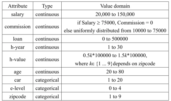
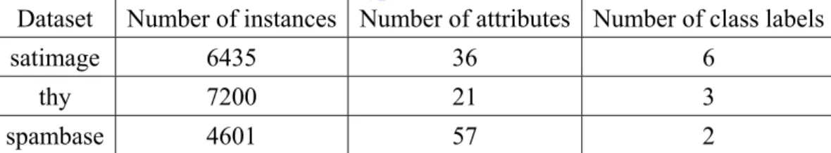
(34) 2.4. UCI Database and IBM Data Generator. In this dissertation, we use both real and synthetic datasets to carry out a series of experimental evaluations. The real experimental datasets are selected from UCI database [59] which is a repository of several kinds of datasets. UCI database is widely used by the machine learning community for the empirical analysis of machine learning algorithms. For artificial experimental datasets, we use IBM data generator [1][2], which was designed by IBM Almaden Research Center and is an open source written by C++ programming language. IBM data generator is a popular tool for researchers to generate artificial data to evaluate the performance of proposed algorithms. One advantage of IBM data generator is that it contains a lot of built-in functions to generate several kinds of datasets, and therefore enable researchers to carry out a series of experimental comparisons. There are nine basic attributes (salary, commission, loan, age, zipcode, h-years, h-value, e-level, and car) and a target attribute in IBM data generator. Among the nine attributes, zipcode, e-level, and car are categorical attributes; and all the others are continuous ones. The number of class labels can be decided by users and is set to 2 as default. The summary of these nine basic attributes are illustrated in Table 2.2. In this dissertation, we modify IBM data generator to generate datasets containing concept-drifting records.. 21.

(35) Table 2.2 The summary of nine basic attributes in IBM data generator Attribute. Type. Value domain. salary. continuous. 20,000 to 150,000. commission continuous. if Salary ≥ 75000, Commission = 0 else uniformly distributed from 10000 to 75000. loan. continuous. 0 to 500000. h-year. continuous. 1 to 30. h-value. continuous. age. continuous. 20 to 80. car. categorical. 1 to 20. e-level. categorical. 0 to 4. zipcode. categorical. 1 to 9. 0.5k*100000 to 1.5k*100000, where k∈{1 ... 9}depends on zipcode. 22.

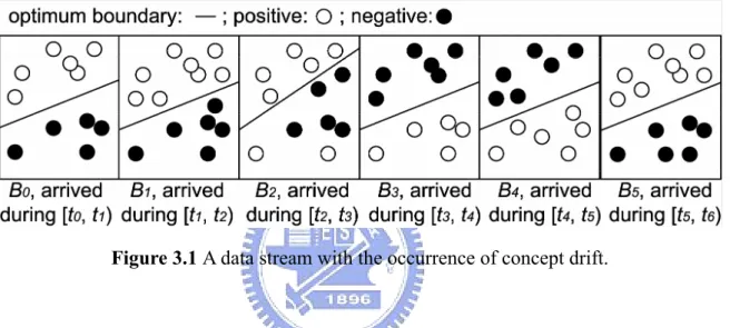
(36) Chapter 3 Sensitive Concept Drift Probing Decision Tree Algorithm. In this chapter, we first give some formal discussions of the concept-drifting problem in Section 3.1. In Section 3.2, we introduce our sensitive concept drift probing decision tree algorithm (SCRIPT). The empirical analyses of SCRIPT are presented in Section 3.3.. 3.1. One-way Drift and Two-way Drift. To make readers easily understand the problem we will address later, in this dissertation we divide the concept drift into concept stable, concept drift and concept shift. We refer to the examples in [73] and modify the figures to illustrate the problem in Figure 3.1. Figure 3.1 represents a two-dimensional data stream and is divided into six successive data blocks according to the arriving time of data. Instances arriving between ti and ti+1 form block Bi, and the separating line in each block stands for the optimum classification boundary in this block. During time t0 to t1, data blocks B0 and B1 have similar data distribution. That is, data stream during this period is stable. Thereafter in B2, some instances shows concept drift and the optimum boundary changes. This is defined as concept drift. Finally, data blocks B4 and B5. 23.

(37) have opposite sample distribution and this is defined as concept shift. Obviously, since the sample distributions of the first two blocks B0 and B1 are quite close, we can use decision tree DT0 built by B0 as the classifier for B1 to save the computational and recording cost. Meanwhile, B2 shows slight differences when compared with the sample distribution of B1 and an efficient approach should make correction according to the original decision tree in stead of rebuilding it.. Figure 3.1 A data stream with the occurrence of concept drift.. In Section 2.2, we have showed that past proposed solutions are not sensible enough to the drifting concepts. That is, the proposed solutions can detect the changes until the number of drifting instances reaches a threshold to cause obvious difference in accuracy or information gain or gini index. Here we describe another concept drift problem which would enforce some proposed solutions such as CVFDT and DNW make a wrong prediction. In order to introduce this problem, we subdivide concept drift into one-way drift and two-way drift. Take Figure 3.1 as the example again, we can find that some negative data in B2 drift to be positive data in B3, known as one-way drift. However, the positive data in B4 drift to be negative in B5, and vice versa, known as two-way drift. We can regard two-way drift as a kind of “local” concept shift if it occurs in the internal or leaf node of a decision tree. If the variation of information gain or gini index is used as the criterion to judge the occurrence of. 24.

(38) concept drift, e.g. the difference of information gain adopted in CVFDT, we can detect only one-way drift since the information gain obtained from B4 would the same as B5. It is worth to note that for the real data, two-way drift might happen. For example, a hacker in turn uses two computers with IP address x and y to send attack packages. When an internal node, which is learned from the first data block, splits the packages form x as safe and that from y as attack, there might be a contrary result learned from another data block. A similar condition might be found in trash mail protection, image comparison and so on.. 25.

(39) 3.2. Sensitive Concept Drift Probing Decision Tree Algorithm. 3.2.1. Class Distribution on Attribute Value. Since the proposed solutions to mine concept-drifting data stream check the occurrence of concept drift on the level of instance or attribute, they generally are not sensitive enough. Besides, they are also unable to detect the two-way drift illustrated in Figure 3.1. To solve these problems, SCRIPT probe the changes at a more detailed level, which is called Class Distribution on Attribute Values (CDAV) and defined as follows.. Definition 3.1: Assuming that a data block contains m target classes ck (k = 1,... ,m), n attributes Ai (i = 1,... ,n), and each attribute ai having v attribute values aij (j = 1,... ,v), then the distribution of target class ck on the attribute value aij is defined as a CDAVij (Class Distribution on Attribute Value).. With Definition 3.1, we can use the chi-square (X2) test to check if there are concept drifts between two data blocks. X2 test is a statistical measure used to test the hypothesis that two discrete attributes are statistically independent. Applied to the concept-drifting problem, it tests the hypothesis that the class distribution on an attribute value of two data blocks is identical. The formula to computing the X2 value is. X2 =. ( f 'ijk − f ijk ) 2. (3.1). f ijk. , where fijk represents the number of instances having attribute value aij and class ck in D and f’ijk is that in D’. With Formula 3.1, we can then define the variance of a CDAVij in the two data blocks as follows. 26.

(40) Definition 3.2: For a given significant level α, the variance CDAVD→ D ' (i, j ) of the a CDAVij between two data blocks D and D’ in a data stream is defined as m. ( f 'ijk − f ijk ) 2. k =1. f ijk. CDAVD→ D ' (i, j ) = ∑. .. (3.2). Proposition 3.1: For the two data blocks D and D’ , if all CDAVD→ D ' (i, j ) < ε, then the concept distribution on all attribute value aij in the two data blocks show no significant difference, and neither do the accuracy of decision tree built according to D and D’, respectively. Proof: Since CDAVD→ D ' (i, j ) < ε, we can obtain fijk ≅ f’ijk for target classes ck (k = 1,... ,m), attributes Ai (i = 1,... ,n) and attribute value aij. For attribute Ai, the Entropy before the splitting is m. I(Ai) = − ∑ Pik log Pik , k =1. where Pik = fi+k / N, fi+k denotes the total number of instances belonging to class ck as shown in Table 3.1, and N denotes the total number of instances in the data block. Since fijk ≅ f’ijk and N = N’ we can obtain v. v. j =1. j =1. Pik = fi+k / N = ∑ f ijk / N ≅ −∑ f ijk' / N ' = f i +' k / N ' = P’ik. Continually, we can obtain that m. m. k =1. k =1. − ∑ Pik log Pik ≅ −∑ Pik' log Pik' and. I ( Ai ) ≅ I ( Ai' ) .. (3.3). That is, the Entropy of attribute ai before splitting in data blocks D and D’ is similar. Suppose we splitting all instances N into v subset by attribute Ai, the Entropy of attribute Ai. 27.

(41) after splitting is v. f ij +. j =1. N. E(Ai) = ∑. m. × (−∑ Pijk log Pijk ) ,. (3.4). k =1. where Pijk = fijk / fij+, fij+ denotes the total number of instances having attribute value aij as shown in Table 3.1. Since fijk ≅ f’ijk we can infer that for the attribute value aij fij+ ≅ f’ij+.. (3.5). As a result, we can also obtain that m. m. k =1. k =1. Pijk ≅ P’ijk and − ∑ Pijk log Pijk =≅ −∑ Pijk' log Pijk'. (3.6). From Formulas (3.4), (3.5) and (3.6), we can get that E ( Ai ) ≅ E ( Ai' ) .. (3.7). From Formulas (3.3) and (3.7), we can get that Gain( Ai ) = I ( Ai ) − E ( Ai ) ≅ I ( Ai' ) − E ( Ai' ) = Gain( Ai' ) . That is, the Information gain of attribute Ai in data blocks D and D’ is similar. As a result, the two decision trees which are respectively built by using blocks D and D’ will be similar.. ■. Table 3.1 The class label distribution on an attribute Ai. Class label \ value. ai1. ai2. c1 c2. fi11 fi12. fi21 fi22. M cm. M. M. fi1m. Summation. fi1+. …. aiv. Summation. fiv1 fiv2. fi+1 fi+2. M. M. fi21. fivm. fi+m. fi2+. fiv+. N. M. By Proposition 3.1 and Formula 3.2, we can detect any kind of concept drift between two data blocks and then build an accurate decision tree. The significance level can be set to be. 28.

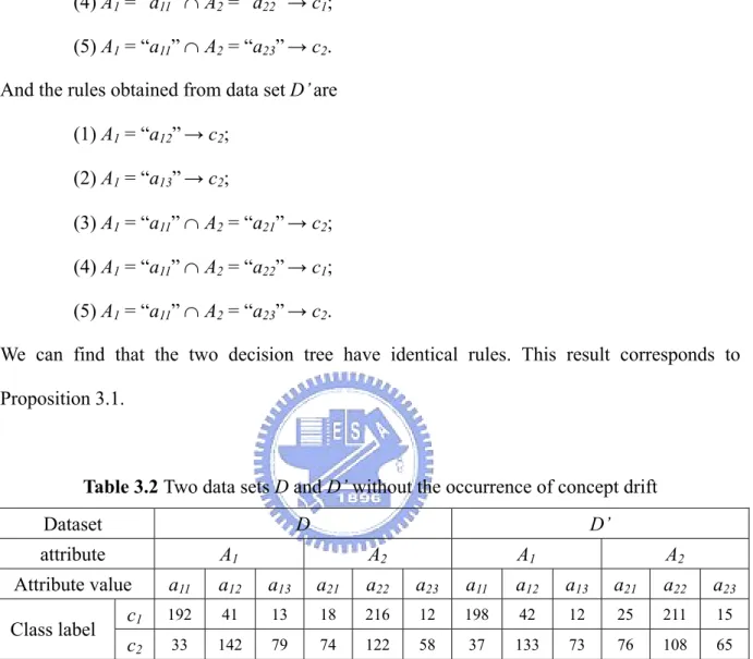
(42) smaller or larger according to the needs of applications. With a given significance level, we can obtain the ε by checking the X2 table in a statistical book. The degree of freedom will be 1 less than the number of classes. Suppose that we set the level of significance α = 5% and there are three classes, if all CDAVD → D ' (i, j ) are less than ε = 5.991, that means the class distribution on all attributes shows no significant difference between D and D’ with 95% confidence. As a result, the information gain obtained from any attribute will show no significant difference and the decision tree need not to be rebuilt. Note that the purpose of Proposition 3.1 is to claim that a rebuild tree will have very similar accuracy to that of original one, rather than to guarantee the rebuild tree will be a copy of the original one.. Example 3.1: For clearly understand our idea, a case with two datasets D and D’ is presented. in Table 3.2. Each of the two sets has two attributes A1 and A2, and each attribute has three attribute values (a11, a12, a13; a21, a22, a23). There are total 500 instances and two classes are c1 and c2 in each dataset. Assuming that the level of significance α =5% (degree of freedom = 1 and ε = 3.841), we can infer the following by Formula 3.2: CDAVD→D＇ (1,1) = 0.6723 < ε ; CDAVD→D＇ (1,2) = 0.5948 < ε ; CDAVD→D＇ (1,3) = 0.5326 < ε ; CDAVD→D＇ (2,1) = 2.7763 < ε ; CDAVD→D＇ (2,2) = 1.7223 < ε ; CDAVD→D＇ (2,3) = 1.5948 < ε . Since all CDAVs have no significant difference, by Proposition 3.1 mentioned above, the decision trees built respectively with D and D’ would be very similar. To verify this, we build the two decision trees and show the corresponding rules. The rules obtained from data set D are (1) A1 = “a12” → c2; 29.

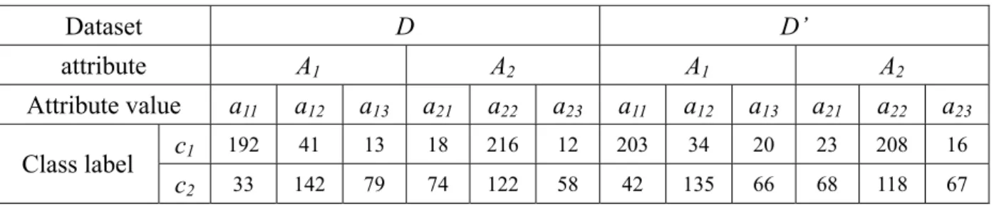
(43) (2) A1 = “a13” → c2; (3) A1 = “a11” ∩ A2 = “a21” → c2; (4) A1 = “a11” ∩ A2 = “a22” → c1; (5) A1 = “a11” ∩ A2 = “a23” → c2. And the rules obtained from data set D’ are (1) A1 = “a12” → c2; (2) A1 = “a13” → c2; (3) A1 = “a11” ∩ A2 = “a21” → c2; (4) A1 = “a11” ∩ A2 = “a22” → c1; (5) A1 = “a11” ∩ A2 = “a23” → c2. We can find that the two decision tree have identical rules. This result corresponds to Proposition 3.1.. Table 3.2 Two data sets D and D’ without the occurrence of concept drift. Dataset. D. attribute. A1. Attribute value Class label. D’ A2. A1. A2. a11. a12. a13. a21. a22. a23. a11. a12. a13. a21. a22. a23. c1. 192. 41. 13. 18. 216. 12. 198. 42. 12. 25. 211. 15. c2. 33. 142. 79. 74. 122. 58. 37. 133. 73. 76. 108. 65. Corollary 3.1: By Proposition 3.1, we can infer that if the variance of CDAV for the two data. blocks D and D’ is greater than or equivalent to a threshold ε, (i.e. CDAVD→D＇ (i,j) ≥ ε), then concept drift may occur between D and D’. As a result, the original decision tree needs to be corrected.. Example 3.2: Here, we use the two datasets in Table 3.3, which is modified from Table 3.2, to. illustrate this Corollary. Again assuming that the level of significant α = 5% (degree of 30.

(44) freedom = 1 and ε = 3.841), we can infer the following by Formula 2: CDAVD→D＇ (1,1) = 3.0848 < ε; CDAVD→D＇ (1,2) = 1.5402 < ε ; CDAVD→D＇ (1,3) = 5.9085 > ε;. CDAVD→D＇ (2,1) = 1.8754 < ε ; CDAVD→D＇ (2,2) = 0.4274 < ε; CDAVD→D＇ (2,3) = 2.7299 < ε Since CDAV13 achieves significant difference, by Corollary 3.1, we can claim that concept drift occurs and the decision trees built respectively with D and D’ would be different. To verify this, we again show the corresponding rules for two trees as follows. The rules obtained from data set D are (1) A1 = “a12” → c2; (2) A1 = “a11” ∩ A2 = “a21” → c2; (3) A1 = “a11” ∩ A2 = “a22 ”→ c1; (4) A1 = “a11” ∩ A2 = “a23 ”→ c2; (5) A1 = “a13” → c2. And the rules obtained from data set D’ are (1) A1 = “a12” → c2; (2) A1 = “a11” ∩ A2 = “a21” → c2; (3) A1 = “a11” ∩ A2 = “a22” → c1; (4) A1 = “a11” ∩ A2 = “a23” → c2; (5) A1 = “a13” ∩ A2 = “a21” → c2; (6) A1 = “a13” ∩ A2 = “a22” → c1; (7) A1 = “a13” ∩ A2 = “a23” → c2. By comparison, we can find that the rule A1 = a13 → c2 in dataset D have some changes in data set D’; the results correspond to our Corollary. 31.

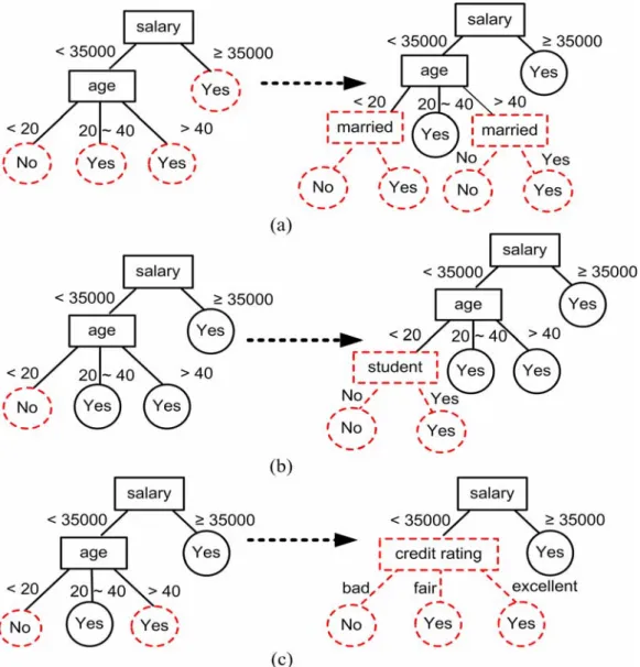
(45) Table 3.3 Two data sets D and D’ with the occurrence of concept drift. Dataset. D. attribute. A1. Attribute value Class label. 3.2.2. D’ A2. A1. A2. a11. a12. a13. a21. a22. a23. a11. a12. a13. a21. a22. a23. c1. 192. 41. 13. 18. 216. 12. 203. 34. 20. 23. 208. 16. c2. 33. 142. 79. 74. 122. 58. 42. 135. 66. 68. 118. 67. Correction Mechanism in SCRIPT. Before we introduce the correction mechanism in SCIPIT, it is worth to note that drifting instances should gather in some specific areas in the dimensional space of attributes, otherwise they can be regarded as noise instances. Accordingly, another advantage of CDAV is that it can reveal which attribute values cause concept drift before building the decision tree by aggregating the drifting CDAVs. This enables SCRIPT to efficiently and immediately amend the original decision tree. For example, we can recognize the concept drift is caused by attribute value a13 in Example 3.2. Therefore, we can only correct the subtree rooted at a13 to efficiently correct the classification model.. Example 3.3: We use Figure 3.2 to further illustrate the idea of correction mechanism in. SCRIPT. Figure 3.2 is a decision tree trained from old customer’s data to predict if a customer will apply for credit cards. For better understanding, only the subtree rooted at attribute “salary” is shown. A similar decision tree, except that it is trained from new customer’s data stream, is shown in Figure 3.2 (b). By comparison with the CDAVs in Figure 3.2 (a) and Figure 3.2 (b), we can find that some concepts in new data block are significantly different from that in old one. More importantly, we can find that these changes gather up in the branch 32.

(46) of “age < 20 and 20 ≤ age < 40”. Accordingly, the aggregated drifting CDAVs is 0 ≤ age < 40 and it means that a people younger than 40 have changed his concepts in this example. To efficiently provide a decision tree suitable for new customers’ data block, we can only correct the subtree rooted at 0 ≤ age < 40 as in Figure 3.2 (b).. (a). (b) Figure 3.2. Two data blocks with the occurrence of concept drift: (a) original data block and. the corresponding sub-tree; (b) new data block and the corresponding sub-tree.. Now, we detail the correction mechanism in SCRIPT. In the processing of data stream, 33.

(47) when the difference of CDAV between new data block Bt and original data block Bt -i (t ≥ i ≥ 1) is greater than the given threshold (the level of significance is set 0.05 as the default), the correction methods in SCRIPT can be divided into the following cases. The corresponding illustration of each case is shown in Figure 3.3. In each case of Figure 3.3, the dotted node in the left tree (original tree) denoted the occurring of concept drift and the dotted subtree in the right tree (new tree) is an alternate tree built by SCRIPT. For each aggregated drifting CDAV in attribute Ai with value(s) aij, a. If attribute Ai is not a splitting attribute of a node in the original decision tree, SCRIPT. will use this attribute to split all leaf nodes by using data block Bt. Such a variation of CDAV indicates that an attribute with originally little information changes into an optimal splitting attribute due to concept drift. We illustrate this condition in Figure 3.3(a). b. If attribute Ai is a splitting attribute of a node in the original decision tree and all. CDAVs group in an interval aij, SCRIPT will remove the subtree rooted at the attribute value aij from the original tree and use data block Bt to build the alternative tree. Such a variation means concept drift is caused by a fixed range aij of the attribute Ai. Take Figure 3.3(b) for example, for the attribute age, those under 20 were originally inclined not to apply for credit cards; however, with the growing consuming ability of students, more and more are applying. c. If attribute Ai is a split attribute of a node in the original decision tree but all CDAVs. are scattered in several interval, SCRIPT will removes the subtree rooted at this attribute Ai from the original tree and use data block Bt to build the alternative tree. Such a variation represents concept drift is caused by the attribute Ai but within multiple ranges of the attribute. For instance, for the attribute of age, people younger than 20 and older than 40 were originally both inclined not to apply for credit cards; however, with the change of payment types, more and more are applying. In this case, 34.

(48) attribute ‘age’, no longer the optimal split attribute, is replaced by attribute ‘credit rating’, according to a test result. This case is illustrated in Figure 3.3(c).. Note that all aggregated drifting CDAVs might distribute among several attributes and SCRIPT will check if they are in the same path in the original tree before the correctness. If two aggregated CDAVs are in the same path, the one locates in the highest level will be reserved and the other will be ignored.. Figure 3.3 The illustrations of the correction mechanism in SCRIPT when concept drift. occurs.. 35.

(49) 3.2.3. The Pseudocode and Computational Complexity of SCRIPT. Here we present the pseudo-code of SCRIPT and analyze its computational complexity. Below is the pseudo code of SCRIPT. Giving the size of data block N and the significance level α, SCRIPT calculates the CDAVs in data block B0 in Line 4 as the initial reference. Note that, N can be set larger in a high speed environment or smaller for the real time application; however, fijk must be larger than 5 which is a basic requirement in X2 statistics test. Similarly, α can be set smaller if the detection of concept drift is very important and larger otherwise. The default significant level α in SCRIPT is set as 0.05 since this value is widely used as the default in statistics. It is not hard to imagine that SCRIPT will be more sensitive to the concept drift but may require more computational cost if we use a larger significant level α; on the contrary, SCRIPT will be more tolerant to the noise data with a smaller α. The CDAVs of new coming block Bt+1 are calculated in Line 7. The CDAVs of two data blocks Bt and Bt+1 are compared in Lines 8 to 11. All drifting CDAVs are then aggregated in Line 13 for the purpose of efficiently correcting the decision model in Lines 19 to 28. The recorded information is updated in Line 29. Finally, the decision tree is output in Line 31.. 36.

(50) SCRIPT Algorithm Inputs: N: the size of the block (1000 as the default);. Bt: the data block in time step t; α: the level of significance (0.05 as the default); SCRIPT (N, α, Bt) /* Initialization */ 1. t = 0; 2. Build the original decision treeDT0 by B0; 3. Record all splitting attributes of DT0 in Splitatt[]; 4. Count the CDAVs in B0 and record them in RCDAV[]; 5. t = t + 1 6. For the new coming data block Bt in time step t Count CDAVijk in NCDAV[]; 7. 8. For each CDAVij in the new data block 9. If | CDAVt-1→t (i, j) | > ε 10. 11. 12. 13. 14. 15. 16. 17. 18. 19. 20. 21. 22. 23. 24. 25. 26. 27. 28. 29. 30. 31.. Record this CDAV in DCDAV[]; End if If DCDAV[] is not empty Aggregate the recorded CDAVs; For all aggregated CDAVs If two aggregated CDAVs are in the same path in the original decision tree Reserve the one locates in the highest level in ACDAV[] ; End if Update ; For all aggregated CDAVs belonged to attribute Ai in ACDAV[] If attribute Ai is not in Splitatt[] Build an alternative tree rooted at this node by using Bt; Elseif attribute Ai is in Splitatt[] and all aggregated CDAVs in ai group in an interval aij Remove the subtree rooted at this attribute value aij from DTt-1; Build the alternative tree rooted at aij by using Bt; Else Remove the subtree rooted at this attribute Ai from DTt-1; Build the alternative tree rooted at Aj by using Bt; End if Update Splitatt[], RCDAV[], and the recorded decision tree; End If Output the decision tree.. 37.

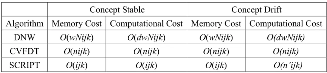
(51) Below, we compare the system cost of SCRIPT to that of two state-of-the-art window-based approaches: DNW and CVFDT. Assumed a data block has i attributes, k class labels, each attribute has j attribute values, since SCRIPT records the referred CDAVs, it has a memory cost O(ijk). SCRIPT also needs to record a decision tree and the splitting attributes in this tree, however, the memory cost is O(n) and can be ignored, where n is the number of nodes of the recorded decision tree. For CVFDT, since it has to record the counting in each node of the recorded decision tree, the memory cost is O(nijk). DNW, which is a sliding window approach, might have a worst record cost since it record instances instead counting and new data blocks might have to be mixed into old ones. If the maintained data is w times as much as that of a new data block, then the memory cost of DNW is O(wNijk), where N is the number of instances in the block. In the aspect of computational cost, while the concept is stable, the required computational cost of SCRIPT is O(ijk). For CVFDT, it has to check the information gain for each attribute in each node of decision tree when a new data block is given. If the tree has n nodes, the computational cost needed would be O(nijk) [38]. For DNW, the computational cost would be O(dwNijk), where d is the depth of the tree, since the tree is rebuilt from scratch. When there is concept drift, DNW and CVFDT have a similar computational cost to that in stable stream. Since SCRIPT directly corrects some sub-trees by checking the drifting CDAVs, the computational cost of the rebuilding is O(ij)+O(n’ijk), where n’ ≤ n and O(ij) is responsible for the comparison of CDAVs and O(n’ijk) is the computational cost for the rebuilding of sub-trees. Comparisons of system cost among SCRIPT, DNW, and CVFDT in stable and drifting data stream are summarized in Table 3.4. In summary, SCRIPT has the smallest memory requirement and computational cost when concept is stable. When concept drifts, SCRIPT still requires the smallest memory cost and a better or comparable computational cost.. 38.

(52) Table 3.4 The Comparisons of system cost among SCRIPT, DNW, and CVFDT. Concept Stable. Concept Drift. Algorithm Memory Cost Computational Cost Memory Cost Computational Cost DNW. O(wNijk). O(dwNijk). O(wNijk). O(dwNijk). CVFDT. O(nijk). O(nijk). O(nijk). O(nijk). SCRIPT. O(ijk). O(ijk). O(ijk). O(n’ijk). 39.