國
立
交
通
大
學
電信工程學系
碩
士
論
文
利用限制隨機賽局在認知網路下動態管理功率
Dynamic Power Management in Cognitive Radio Networks
based on Constrained Stochastic Games
研 究 生:王佳偉
指導教授:方凱田 教授
利用限制隨機賽局在認知網路下動態管理功率
Dynamic Power Management in Cognitive Radio Networks based on Constrained Stochastic Games
研 究 生 :王佳偉 Student:Chia-Wei Wang 指導教授 :方凱田 Advisor:Kai-Ten Feng 國 立 交 通 大 學 電 信 工 程 學 系 碩 士 論 文 A Thesis
Submitted to Department of Communications Engineering College of Electrical and Computer Engineering
National Chiao Tung University in partial Fulfillment of the Requirements
for the Degree of Master of Science
in
Communications Engineering
June 2009
Hsinchu, Taiwan, Republic of China
利用限制隨機賽局在認知網路下動態管理功率 學生:王佳偉 指導教授:方凱田教授 國立交通大學電信工程學系碩士班 摘 要 近年研究指出,已分配頻帶的頻寬使用效率低,而為了促使頻寬使 用效率的提升,認知網路(Cognitive Radio, CR)則被提出來動態的使 用這些已分配卻效率不高的頻帶。其中在認知網路中使用者之間的訊號 干擾與功率分配則被提出許多的相關研究。因此,在這篇論文中,使用 賽局理論(Game Theory)的限制隨機賽局(Constrianed Stochastic Game) 在動態的通道環境與存在頻寬的使用者下,求出此問題的最佳決策。內 容的研究中,分別求出有限時間和無限時間下,包含了已分配與未分配 頻帶的最佳決策。而在求解的過程中,均對信號的干擾做了限制,因此 CR 的使用者對頻寬的擁有者不會造成嚴重的干擾。根據賽局理論模型的 表示,可以證明存在賽局的奈許平衡解(Nash equilibrium),而此奈許 平衡解可以使每個 CR 使用者在彼此競爭的情況下得到個人的最佳化。 在模擬的部分,驗證了確實可達到奈許平衡解,也顯示可優於貪婪式的 演算法(Greedy mechanism),並且對有通道感測的誤差下仍可達到可預 期的結果。
Dynamic Power Management in Cognitive Radio Networks based on Constrained Stochastic Games
student:Chia-Wei Wang Advisors:Dr. Kai-Ten Feng
Department of Communication Engineering National Chiao Tung University
ABSTRACT
Recent studies have been conducted to indicate the ineffective usage of licensed bands due to the static spectrum allocation. In order to improve the spectrum utilization, the cognitive radio is therefore suggested to dynamically exploit the opportunistic primary frequency spectrums. The interference from the secondary users to the primary user consequently draws the attention to the spectrum and power management for the cognitive radio networks. In this paper, the constrained stochastic games are utilized to exploit the optimal policies for power management by considering the variations from both the channel gain and the primary traffic. Both the underlay and overlay waveforms are considered within the network scenarios for the proposed power
management scheme. Constraints for allowable interferences will be applied in order to preserve the communication quality among the primary and the
secondary users. With the assumption of the Markovian property of dynamic environment, finite and infinite time horizon scenarios are both considered in target function. According to the formulation of the constrained stochastic games, the existence of the constrained Nash equilibrium will be validated with rigorous proofs. Simulation results further validate the correctness of the
theoretically-derived policies, compare with the greedy mechanism and examine the effect of channel sensing error for dynamic power management.
誌
謝
回頭看兩年的時間過去就是覺得特別快,但在交通大學的研究生活卻是我難忘的深 刻體驗。畢業典禮的到來讓我開始回想起在這兩年研究的經歷,從一開始的對研究的無 所適從,一步步對研究的探討,到最後論文的完成,都是在 Mint Lab 裡教授、學長和 同學的互相學習上完成的。感謝這個實驗室對我的幫助,也懷念在研究的過程中帶來的 快樂。 這篇論文的完成,要感謝指導教授方凱田老師的教導,在研究的討論與寫作的問題 中,老師總是會很細心的幫助我在研究中所遇到的問題,也能夠給我很大的空間在研究 上發揮,讓我順利完成這篇論文。另外也要感謝研究助理許裕彬學長在研究上的帶領與 學習,在我對研究方向和繁雜的數學推導中,都能給我很大的幫助,也在我遇到困難的 情況中,給我信心去面對問題。祝福你在美國的博士生涯能三年內順利完成。而口試時, 蘇育德老師和黃經堯老師也提供了研究中實現上的問題點與其他寶貴意見,能讓我這篇 論文有更完整的改進,使我明白能藉由不同的觀點去思考研究問題。 在實驗室中,博士班的仲賢學長、建華學長、文俊學長和伯軒學長都曾在研究上給 過我幫助,而更重要的是他們在研究上所表現的態度與專業更讓我明白研究生的模範表 現是如何。而學弟其懋、萬邦、俊宇、承澤和惟能則是研究室的新生力軍,除了為實驗 室帶來更歡樂的氣氛,也從他們身上看到他們對自己的研究所投注的努力與熱情。 同屆的同學瑞廷、俊傑和佳仕,兩年的時間中一起上課、討論、運動,帶來的快樂 和互相幫助,是我研究生涯中愉快的時光。瑞廷的研究和我一樣是 CR,因此在彼此的討 論中就有比較多的互動,外加在實驗室中的座位也在我旁邊,生活上也能更認識到他一 些正面的特質,如流利的英語口說和清楚的語言表達,讓我有深刻的印象。俊傑的優秀 表現,讓我體會到厲害的研究生也可以在研究與生活中取得平衡,而他對同學間的關懷 也讓我感到很溫馨。而佳仕同學和他在修課方面有很多的接觸,讓我感受到他專業與邏 輯上的特長,每次與他討論,都能學到清楚的觀念與知識。相信他在未來的博士生涯, 也會很順利的畢業。心中很感謝也覺得很幸運有這一幫好同學,從你們身上學到太多太 多東西讓我成長。 最後要感謝我的家人,在我離家學習的兩年在背後默默的給我支持,也給了我很大的空 間讓我在學習上能夠更自由,期待未來的日子,盡我所能回報給最愛的家人。 王佳偉謹誌 于新竹國立交通大學
Contents
Chinese Abstract i English Abstract ii Acknowledgement iii Contents iv List of Figures vi 1 Introduction 12 System Model for Dynamic Power Management with
Con-strained Stochastic Games 6
2.1 Finite Time Horizon . . . 9
2.2 Infinite Time Horizon . . . 11
3 Existence of CNE for Finite Time Horizon Stochastic Game 13
3.2 Existence of CNE . . . 16
4 Existence of CNE for Infinite Time Horizon Stochastic Game 19 5 Numerical Evaluation 28 5.1 Finite Time Horizon . . . 30
5.1.1 Validate . . . 30
5.1.2 Compare with greedy mechanism . . . 34
5.2 Infinite Time Horizon . . . 37
5.2.1 Validate . . . 37
5.2.2 Compare with greedy mechanism . . . 41
5.2.3 Effect of channel sensing error . . . 41
List of Figures
2.1 The schematic diagram of the cognitive radio network for
dy-namic power management. (Tx : transmitter , Rx : receiver) . 7
5.1 Finite Time Horizon : Time length versus expected utility
under 𝐶0 = 0.5𝑚𝑊 , 𝐶1 = 0.5𝑚𝑊 and 𝑟𝑖,𝑑𝑎𝑡𝑎 . . . 30
5.2 Finite Time Horizon : Time length versus expected utility
under 𝐶0 = 0.5𝑚𝑊 , 𝐶1 = 1𝑚𝑊 and 𝑟𝑖,𝑑𝑎𝑡𝑎 . . . 31
5.3 Finite Time Horizon : Time length versus expected utility
under 𝐶0 = 0.25𝑚𝑊 , 𝐶1 = 0.5𝑚𝑊 and 𝑟𝑖,𝑑𝑎𝑡𝑎 . . . 31
5.4 Finite Time Horizon : Time length versus expected utility
under 𝐶0 = 0.25𝑚𝑊 , 𝐶1 = 1𝑚𝑊 and 𝑟𝑖,𝑑𝑎𝑡𝑎 . . . 32
5.5 Finite Time Horizon : Time length versus expected
interfer-ence under 𝐶0 = 0.5𝑚𝑊 , 𝐶1 = 0.5𝑚𝑊 and 𝑟𝑖,𝑑𝑎𝑡𝑎 . . . 32
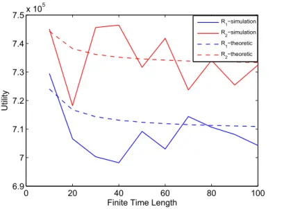
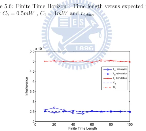
5.6 Finite Time Horizon : Time length versus expected
interfer-ence under 𝐶0 = 0.5𝑚𝑊 , 𝐶1 = 1𝑚𝑊 and 𝑟𝑖,𝑑𝑎𝑡𝑎 . . . 33
5.7 Finite Time Horizon : Time length versus expected
5.8 Finite Time Horizon : Time length versus expected
interfer-ence under 𝐶0 = 0.25𝑚𝑊 , 𝐶1 = 1𝑚𝑊 and 𝑟𝑖,𝑑𝑎𝑡𝑎 . . . 34
5.9 Finite Time Horizon : 𝐶0 versus expected interference under
𝑟𝑖,𝑑𝑎𝑡𝑎 . . . 35
5.10 Finite Time Horizon : 𝐶1 versus expected interference under
𝑟𝑖,𝑑𝑎𝑡𝑎 . . . 35
5.11 Finite Time Horizon : 𝐶0 versus expected interference under
𝑟𝑖,𝑝𝑟𝑖𝑐𝑖𝑛𝑔 . . . 36
5.12 Finite Time Horizon : 𝐶1 versus expected interference under
𝑟𝑖,𝑝𝑟𝑖𝑐𝑖𝑛𝑔 . . . 36
5.13 Infinite Time Horizon : Time length versus expected utility
under 𝐶0 = 0.5𝑚𝑊 , 𝐶1 = 0.5𝑚𝑊 and 𝑟𝑖,𝑑𝑎𝑡𝑎 . . . 37
5.14 Infinite Time Horizon : Time length versus expected utility
under 𝐶0 = 0.5𝑚𝑊 , 𝐶1 = 1𝑚𝑊 and 𝑟𝑖,𝑑𝑎𝑡𝑎 . . . 38
5.15 Infinite Time Horizon : Time length versus expected utility
under 𝐶0 = 0.25𝑚𝑊 , 𝐶1 = 0.5𝑚𝑊 and 𝑟𝑖,𝑑𝑎𝑡𝑎 . . . 38
5.16 Infinite Time Horizon : Time length versus expected utility
under 𝐶0 = 0.25𝑚𝑊 , 𝐶1 = 1𝑚𝑊 and 𝑟𝑖,𝑑𝑎𝑡𝑎 . . . 39
5.17 Infinite Time Horizon : Time length versus expected
interfer-ence under 𝐶0 = 0.5𝑚𝑊 , 𝐶1 = 0.5𝑚𝑊 and 𝑟𝑖,𝑝𝑟𝑖𝑐𝑖𝑛𝑔 . . . 39
5.18 Infinite Time Horizon : Time length versus expected
5.19 Infinite Time Horizon : Time length versus expected
interfer-ence under 𝐶0 = 0.25𝑚𝑊 , 𝐶1 = 0.5𝑚𝑊 and 𝑟𝑖,𝑝𝑟𝑖𝑐𝑖𝑛𝑔 . . . 40
5.20 Infinite Time Horizon : Time length versus expected
interfer-ence under 𝐶0 = 0.25𝑚𝑊 , 𝐶1 = 1𝑚𝑊 and 𝑟𝑖,𝑝𝑟𝑖𝑐𝑖𝑛𝑔 . . . 41
5.21 Infinite Time Horizon : 𝐶0 versus expected interference under
𝑟𝑖,𝑑𝑎𝑡𝑎 . . . 42
5.22 Infinite Time Horizon : 𝐶1 versus expected interference under
𝑟𝑖,𝑑𝑎𝑡𝑎 . . . 42
5.23 Infinite Time Horizon : 𝐶0 versus expected interference under
𝑟𝑖,𝑝𝑟𝑖𝑐𝑖𝑛𝑔 . . . 43
5.24 Infinite Time Horizon : 𝐶1 versus expected interference under
𝑟𝑖,𝑝𝑟𝑖𝑐𝑖𝑛𝑔 . . . 43
5.25 Infinite Time Horizon : error percent versus expected
interfer-ence under 𝑟𝑖,𝑑𝑎𝑡𝑎 . . . 44
5.26 Infinite Time Horizon : error percent versus expected
Chapter 1
Introduction
Due to rapid development of wireless systems, the demand for wireless spec-trums has resulted in spectrum scarcity based on the conventional fixed al-location schemes. Even with the intensive usage of frequency spectrums, it has been studied by extensive measurements [1] that 62% of spectrum still remains unoccupied by the licensed primary user (PU). Cognitive radio (CR) is an intelligent wireless communication system that is perceptible to its sur-roundings. It is advanced as an emerging technology to effectively exploit the under-utilized spectrum in order to overcome the overcrowded spectrum problem.
There are two types of spectrum sharing that are defined for the CR networks (CRNs), including the underlay and the overlay waveforms. The underlay waveform represents that the unlicensed secondary users (SUs) are allowed to simultaneously share the primary frequency spectrum with the
PUs. The transmission power of the SUs are in general limited in order not to cause excessive interferences to the PUs. On the other hand, an overlay waveform allows the SUs to perform packet transmission under the existence of a spectrum hole. The spectrum hole is defined as a frequency band au-thorized to PUs, however, it is vacant at a particular time and geographic location. With the overlay waveform, the SUs can sense and identify the existence of spectrum hole for data communications. Therefore, spectrum utilization can be enhanced with these frequency-agile features. The research work in the CRNs has been investigated from various aspects. The work pro-posed in [2; 3] presents the techniques for spectrum sensing and detection; while [4; 5] investigate the spectrum allocation problem for the CR. There are also research [6; 7] focusing on the medium access control design for the CRNs.
Game theory [8] has been considered a feasible mathematical tool for solv-ing the resource allocation problems in distributed CRNs. The fundamental concept of game theory is to resolve the conflict and cooperation between intelligent rational decision-makers (DMs). Instead of reaching a globally optimized solution based on identical objective, the DMs within the gaming formulation are seeking for solutions selfishly without the knowledge of other DMs’ decisions. The primary reason is due to the inherent conflicts between the objectives that are assigned among the DMs, which can be adopted to model the behaviors of both PUs and SUs within the CRNs. After reaching the optimized solution (i.e. Nash equilibrium (NE) [8]) based on the game
theory, each individual DM will not benefit from any action to deviate from the NE. In other words, by considering the conflicted interests between the DMs, the solutions obtained at the NE will provide every DM to possess the optimal resource allocation.
In general, two different types of games are categorized for the game theory, i.e. the strategic games and the extensive games. With the objective of reaching the NE, all DMs simultaneously select their strategies only for one-time by adopting the strategic games [8], which have been exploited to resolve the power control problem for the CRNs in recent research work [9; 10]. The work in [9] proposed an algorithm for distributed multi-channel power allocation based on the strategic gaming model;while the pricing-based games are utilized in [10] to achieve a higher signal-to-noise ratio with the guarantee of reliable data transmissions. However, computation of NEs in strategic game will introduce some computation time at each time.
On the other hand, the extensive games [8; 11; 12] represent a class of gaming models where the DMs repeatedly conduct decision-making numer-ous times for resource allocation. Unlike the strategic games that each DM considers his strategy only at the beginning of the game, the extensive games is implemented whenever a decision has to be made in order to increases the spectrum efficiency by the multi-stage gaming model. The scheme proposed in [12] utilized the repeated game to solve NE point under underlay wave-form. But it can’t character the variation of CRN environment. In addition, constrained stochastic games [13; 14] are formulated by extending the
exten-sive games for dynamically-changing environments with the consideration of certain constraints for optimization. It can be considered as an extension of the Markov decision process from a single DM to multiple DMs. The power allocation algorithm proposed in [15] imposes both the power and the buffer length constraints under the environments with varying channel states. It is noticed that only independent states between the DMs are considered in [15], i.e. the states of power and buffer length for each DM is independent to those from other DMs. So, constrained stochastic games can be applied to the resource management problems for CRNs.
In this paper, the constrained stochastic games are adopted and extended to study the dynamic power management problem in CRNs. The dynamic environments occurred from the channel variations and the uncertain spec-trum holes will be modeled as the ergodic Markov decision process. It is noticed that the spectrum holes are considered the dependent states for each SU since the SUs are sharing to utilize the spectrum holes while the original licensed PU is temporarily releasing the frequency band. Moreover, each SU can perceive its own current state but is unaware of the states and strate-gies from the other SUs. As the licensed spectrum is occupied by the PUs, the underlay waveform is executed by the SUs with the introduction of rea-sonable interferences to the PUs. On the other hand, the SUs will share the spectrum hole with the overlay waveform as the primary traffic is ab-sent. Constraints for allowable interferences will also be imposed to preserve the communication quality among the SUs under the existence of spectrum
holes. With the satisfaction of the defined constraints, the constrained NE suggests an optimal solution to the dynamic power assignment according to the SUs’ current state within the CRNs. In finite and infinite time horizon, i.e.time non-converge and converge to stable point respectively , existence of constrained NE will be proved.
Therefore, considering all of the issues mentioned above, two stochastic game are proposed in this paper to describe the finite time and infinite time horizon respectively in the CRNs. Similar Dynamic programming method will prove the existence of constrained NE in finite time horizon. Using the stable property of CRNs the existence of constrained NE will be demon-strated in infinite time horizon.
The rest of this paper is organized as follows. chapter 2 presents the system models of finite and infinite time horizon of CRNs. The correspond-ing proofs for the existence of constrained Nash equilibrium are provided in chapter 3 and chapter 4 respectively. Numerical evaluation is performed in chapter 5; while chapter 6 draws the conclusions.
Chapter 2
System Model for Dynamic
Power Management with
Constrained Stochastic Games
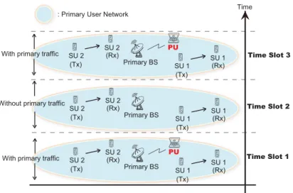
The schematic diagram of the CRN is illustrated in Fig. 2.1, where a syn-chronous slotted time structure is considered. A PU is communicating with its primary base station; while there exists 𝑁 = 2 SU pairs where SU(Tx) is intending to transmit its data packets to the respective SU(Rx) within the same frequency spectrum as the PU. The overlay waveform is shown at the time slot 2 where a spectrum hole happens for the SUs to share the licensed band without the existence of the PU. At both time slots 1 and 3, with toler-able interferences to the PU, the SUs coexist with the PU to conducts their transmissions under the execution of the underlay waveform.Primary BS
Time : Primary User Network
Without primary traffic With primary traffic
Time Slot 1 Time Slot 2 Time Slot 3 PU SU 1 SU 1 (Tx) (Rx) SU 2 SU 2 (Tx) (Rx) Primary BS SU 1 SU 1 (Tx) (Rx) SU 2 SU 2 (Tx) (Rx) Primary BS With primary traffic PU
SU 1 SU 1 (Tx) (Rx) SU 2 SU 2 (Tx) (Rx)
Figure 2.1: The schematic diagram of the cognitive radio network for dynamic power management. (Tx : transmitter , Rx : receiver)
At each time slot 𝑡, each SU(Tx) 𝑖 forwards its data packets with a specific
power level 𝑝𝑡
𝑖 ∈ 𝒑𝑖 ≜ {𝑝𝑖,0, 𝑝𝑖,1, ⋅ ⋅ ⋅ , 𝑝𝑖,max}, which is referred as the action
set in the game theory. The global set of the power level for the entire CRN
is denoted as P = ∏𝑁𝑖=1𝒑𝑖. The dynamic environment in CRN is modeled
as an ergodic Markov chain [16], where feedback information is considered available for each SU pair, i.e. from SU(Rx) to SU(Tx). In other words, each SU(Tx) will possess the information about all the current states that
are detected by its corresponding SU(Rx). The compound state 𝑠𝑡
𝑖 of each SU
𝑖 at the time slot 𝑡 is constructed by two elements 𝜙𝑡
𝑖 and 𝑔𝑖𝑡, i.e. 𝑠𝑡𝑖 = (𝜙𝑡𝑖, 𝑔𝑡𝑖).
The parameter 𝜙𝑡
𝑖 ∈ 𝝓𝑖 ≜ {0, 1} is utilized to denoted the status of the
PU, where 𝜙𝑡
𝑖 = 0 indicates the absence of the primary traffic, and 𝜙𝑡𝑖 = 1
represents the existence of the PU within the CRN. It is noted that, at each
time slot 𝑡, the indication of the primary traffic 𝜙𝑡
𝑖 is considered equal for
can be obtained as Φ =∏𝑁𝑖 𝝓𝑖 = {𝛼, ⋅ ⋅ ⋅ , 𝛼}, where Φ has 𝑁 elements with
𝛼 ∈ {0, 1}. Moreover, the state of the channel gain for each SU 𝑖 at time slot 𝑡 is denoted by the index 𝑔𝑡
𝑖 ∈ 𝒈𝑖 ≜ {0, ⋅ ⋅ ⋅ , 𝐿𝑖 − 1}. The compound state 𝑠𝑡𝑖
will therefore belong to the set 𝒔𝑖 = 𝝓𝑖 × 𝒈𝑖 with the length of state vector
equal to 2𝐿𝑖. The global state space of 𝑠𝑡𝑖 considering all the 𝑁 SUs can also
be represented as S = ∏𝑁𝑖=1𝒔𝑖. The immediate utility of SU 𝑖 is defined as
𝑟𝑖 which is a function of (𝒔𝑡, 𝒑𝑡). Furthermore, 𝑃𝑥𝑦𝑖 = ℳ(𝑠𝑡+1𝑖 = 𝑦∣𝑠𝑡𝑖 = 𝑥)
is utilized to express the state transition probability, where ℳ(𝜀) is the probability measure over an event 𝜀.
A history at time epoch 𝑡 of SU 𝑖 is a time sequence of its current
state as well as its previous states and actions, which is denoted as 𝒉𝑡
𝑖 =
(𝑠0
𝑖, 𝑝0𝑖, 𝑠1𝑖, 𝑝1𝑖, ⋅ ⋅ ⋅ , 𝑠𝑡−1𝑖 , 𝑝𝑡−1𝑖 , 𝑠𝑡𝑖) with 𝑠𝑘𝑖 ∈ 𝒔𝑖 and 𝑝𝑘𝑖 ∈ 𝒑𝑖. Let H𝑡𝑖 be the
col-lection of all possible histories of length 𝑡 for SU 𝑖. A policy employed by SU 𝑖 can be denoted as a sequence 𝒖𝑖 = (𝑢0𝑖, 𝑢1𝑖, ⋅ ⋅ ⋅ , 𝑢𝑖𝑡), where 𝑢𝑡𝑖 : H𝑡𝑖 → ℳ(𝒑𝑖)
is a function mapping from the histories to the probability measure over
the action sets of SU 𝑖. The elements within the policy 𝑢𝑡
𝑖 indicate the
oc-curring probabilities for their corresponding power level 𝑝𝑖,𝑗 for 𝑗 = 0 to
max. It is noted that the decision of the policy 𝑢𝑡
𝑖 for each SU is
indepen-dent to that for the other SUs. The set of all reasonable policies for SU 𝑖 is in the policy space U𝑖, i.e. 𝒖𝑖 ∈ U𝑖. Therefore, with the
considera-tion of all the 𝑁 SUs, the global policy space U = ∏𝑁𝑖=1U𝑖 is called the
class of multi-policies. In addition, the multi-policy except SU 𝑖 is defined as 𝒖−𝑖 = (𝒖1, 𝒖2, ⋅ ⋅ ⋅ , 𝒖𝑖−1, 𝒖𝑖+1, ⋅ ⋅ ⋅ , 𝒖𝑁) ∈ 𝑼−𝑖. Moreover, the stationary
policies are characterized as the policy that is independent of the histories,
i.e. 𝑢𝑡
𝑖 : 𝒔𝑖 → ℳ(𝒑𝑖) as a function mapping only from the current state
𝒔𝑖. The union of all possible stationary policies is denoted as U𝑆𝑖 ∈ U𝑖, and
U𝑆 = ∏𝑁
𝑖=1U𝑆𝑖 ∈ U represents the class of stationary multi-policies.
2.1 Finite Time Horizon
The expected utility of SU 𝑖 with the policy 𝒖 = (𝒖1, 𝒖2, ⋅ ⋅ ⋅ , 𝒖𝑁) ∈ U and
the initial state 𝒔0 = (𝑠0
1, 𝑠02, ⋅ ⋅ ⋅ , 𝑠0𝑁) ∈ S can be obtained as 𝑅𝑇 𝑖 (𝒔0, 𝒖) = 𝑇1 𝑇 −1 ∑ 𝑡=0 𝐸𝒖 𝒔0 [ 𝑟𝑖(𝒔𝑡, 𝒑𝑡) ] (2.1) where 𝐸𝒖
𝒔0 is the operator for the computation of expectation value.
Further-more, the allowable interferences between the SUs and the PU are considered in order to guarantee the quality of service (QoS) of the CRN. The supreme expected allowable interference at the SU i(Rx) is obtained as
𝐼𝑇 𝑖,𝑚(𝒔0, 𝒖) = ∑𝑇 −1 1 𝑡=0 𝐸𝑠0 [ 𝛿0(𝜙𝑡𝑖) ]∑𝑇 −1 𝑡=0 𝑁 ∑ 𝑘=1 𝑘∕=𝑚 𝐸𝒖 𝒔0 [ 𝑝𝑡 𝑘 ⋅ 𝜈𝑘𝑚(𝑠𝑡𝑘) ⋅ 𝛿0(𝜙𝑡𝑘) ] ∀𝑚 ∕= 𝑖 (2.2)
and 𝐼𝑇 𝑝(𝒔0, 𝒖) = ∑𝑇 −1 1 𝑡=0 𝐸𝑠0 [ 𝛿1(𝜙𝑡𝑖) ]𝑇 −1∑ 𝑡=0 𝑁 ∑ 𝑘=1 𝐸𝒖 𝒔0 [ 𝑝𝑡 𝑘⋅ 𝜈𝑘𝑝(𝑠𝑡𝑘) ⋅ 𝛿1(𝜙𝑡𝑘) ] ∀𝑝 ∈ {1, ⋅ ⋅ ⋅ , 𝑀} (2.3)
where 𝛿 is the Kronecker delta function. The function 𝜈𝑘𝑚(𝑠𝑡𝑘) and 𝜈𝑘𝑝(𝑠𝑡𝑘)
represent the corresponding channel gains from SU j(Tx) to SU i(Rx) and
SU j(Tx) to PU in state 𝑠𝑡
𝑘 respectively. In (2.7), 𝐼𝑖,𝑚𝑇 (𝒔0, 𝒖) indicates the
case with the absence of primary traffic, i.e. 𝛿0(𝜙𝑡𝑖 = 0) = 1; while 𝐼𝑝𝑇(𝒔0, 𝒖)
denotes the case with primary traffic, i.e. 𝛿1(𝜙𝑡𝑖 = 1) = 1. Under the usage of
licensed band from PU, the influence occurred from the SUs is confined by 𝐼𝑇
𝑝(𝒔0, 𝒖) ≤ 𝐶1 to assure the QoSof the PU, where 𝐶1 denotes the the PU’s
tolerable interference. Considering the case without the primary traffic, the
allowable interference between the SUs are constrained by 𝐼𝑇
𝑖,𝑚(𝒔0, 𝒖) ≤ 𝐶0,
where 𝐶0 indicates the QoSconstraint among the SUs that share the common
spectrum band. Therefore, the set of feasible policies can be defined as 𝒖 ∈ U
in order to satisfy the condition 𝐼𝑇
𝑖,𝑚(𝒔0, 𝒖) ≤ 𝐶0 ∀𝑚 ∕= 𝑖 and 𝐼𝑝𝑇(𝒔0, 𝒖) ≤
𝐶1 ∀𝑝.
Definition 1. A multi-policy 𝒖∗ = (𝒖∗
1, 𝒖∗2, ⋅ ⋅ ⋅ , 𝒖∗𝑁) ∈ U is a constrained
Nash equilibrium (CNE) if it is a feasible policy such that for all SUs 𝑖 𝑅𝑇
for any feasible policies [𝒖∗
−𝑖∣𝒗𝑖], where the policy [𝒖∗−𝑖∣𝒗𝑖] means that SU 𝑖
uses the policy 𝒗𝑖 while other SUs 𝑘 ∕= 𝑖 takes the policy 𝒖∗𝑘.
2.2 Infinite Time Horizon
The expected utility of SU 𝑖 is 𝑅𝑖(𝒔0, 𝒖) = lim 𝑇 →∞𝑠𝑢𝑝 1 𝑇 𝑇 −1 ∑ 𝑡=0 𝐸𝒖 𝒔0 [ 𝑟𝑖(𝒔𝑡, 𝒑𝑡)] (2.5)
The expected allowable interference at the SU i(Rx) are 𝐼𝑖,𝑚(𝒔0, 𝒖) = lim 𝑇 →∞𝑠𝑢𝑝 1 ∑𝑇 −1 𝑡=0 𝐸𝑠0 [ 𝛿0(𝜙𝑡𝑖) ]⋅ 𝑇 −1 ∑ 𝑡=0 𝑁 ∑ 𝑘=1 𝑘∕=𝑚 𝐸𝒖 𝒔0 [ 𝑝𝑡 𝑘⋅ 𝜈𝑘𝑚(𝑠𝑡𝑘) ⋅ 𝛿0(𝜙𝑡𝑘) ] ∀𝑚 ∕= 𝑖 (2.6) and 𝐼𝑝(𝒔0, 𝒖) = lim𝑇 →∞𝑠𝑢𝑝∑𝑇 −1 1 𝑡=0 𝐸𝑠0 [ 𝛿1(𝜙𝑡𝑖) ]⋅ 𝑇 −1 ∑ 𝑡=0 𝑁 ∑ 𝑘=1 𝐸𝒖 𝒔0 [ 𝑝𝑡 𝑘 ⋅ 𝜈𝑘𝑝(𝑠𝑡𝑘) ⋅ 𝛿1(𝜙𝑡𝑘) ] ∀𝑝 ∈ {1, ⋅ ⋅ ⋅ , 𝑀} (2.7) A multi-policy 𝒖∗ = (𝒖∗
horizon if it is a feasible policy such that for all SUs 𝑖
𝑅𝑖(𝒔0, 𝒖∗) ≥ 𝑅𝑖(𝒔0, [𝒖∗−𝑖∣𝒗𝑖]) (2.8)
It is considered that the SUs are rational [8] such that all SUs are in-tending to maximize their corresponding utilities in (2.5). Furthermore, the
decision for each SU 𝑖 to transmit packets with the power level 𝑝𝑡
𝑖 at the
beginning of time slot 𝑡 is determined without additional knowledge about the states and actions from the other SUs. As a result, the constrained Nash equilibrium (CNE) [14] will be utilized to facilitate the power management problem from the perspective of game theory, which is defined as follows.
The purpose of this paper is to provide the mechanism for dynamic power management based on the optimal polices that are derived from the CNE. The existence of CNE for the finite and infinite time horizon problems will be acquired in chapter III and IV respectively.
Chapter 3
Existence of CNE for Finite
Time Horizon Stochastic Game
In this chapter, the constrained optimization problem with finite time horizon considering a single SU will be introduced in Problem 1. The Markov strategy which will be defined in Definition 2 is also a CNE. The similar dynamic programming method will prove existence of CNE from time slot 𝑇 − 1 to 0 sequentially.3.1 Expected Utility and Markov Strategy
The expected utility of SU 𝑖 when deciding in time slot t is 1 𝑇 − 𝑡 𝑟𝑖(𝒔𝑡, 𝒑𝑡) + ∑ 𝑠𝑡+1 𝑉𝑖(𝑡+1)(𝑠𝑡+1)𝑃𝑠𝑡𝑠𝑡+1 ) (3.1)
where 𝑠𝑡is the state that occurs in time slot t and 𝑃
𝑠𝑡𝑠𝑡+1 is the state transition
probability from 𝑠𝑡 to 𝑠𝑡+1. 𝑉
𝑖(𝑡+1)(𝑠𝑡+1) is the utility that SU 𝑖 expects to
receive in the future starting from time t+1.
Problem 1 (Constrained Optimization Problem (COP) With Finite Time
Horizon). Given a fixed set of policies 𝒖−𝑖 ∈ U−𝑖, find an optimal policy 𝒗∗𝑖
for SU 𝑖 in order to maximize the expected utility 𝑅𝑇 𝑖 (𝒔0, [𝒖−𝑖∣𝒗𝑖]) (3.2) subject to 𝐼𝑇 𝑖,𝑚(𝒔0, [𝒖−𝑖∣𝒗𝑖]) ≤ 𝐶0 ∀𝑚 ∕= 𝑖 (3.3) and 𝐼𝑇 𝑝(𝒔0, [𝒖−𝑖∣𝒗𝑖]) ≤ 𝐶1 ∀𝑝 ∈ {1, ⋅ ⋅ ⋅ , 𝑀} (3.4)
For a COP with finite time horizon with terminal time T expected utility of SU 𝑖 from the strategy combination 𝑢 is given by
where the first term on the right-hand side of the equation is the expected utility using the strategy 𝑢 in time slot 0, the second term is the expected utility from using the strategy 𝑢 in time slot 0 and 1 and so on till the last term which is the expected utility in time slot T-1 when using the strategy
𝑢 throughout the game. Next, defined a special strategies, namely Markov strategies.
Definition 2. A Markov strategy for SU 𝑖 denoted by 𝑢𝑖,𝑀𝑎𝑟 is a sequence
{𝑢𝑡
𝑖,𝑀𝑎𝑟}𝑇𝑡=0 such that 𝑢𝑡𝑖,𝑀𝑎𝑟 : 𝑠𝑡𝑖 → ℳ(𝒑𝑖) is measurable for every t. A
Markov strategy combination 𝑢𝑀𝑎𝑟 is a combination of Markov strategies.
Since Markov strategies restrict SUs to make their decisions conditional only on the current self state, this can be a fairly severe restriction on the kind of strategies SUs can use. However, with the assumptions of Markovian nature of transition probabilities, a SU can do just as well by using a Markov strategy. This is so because the current and future utility of a SU is given by
(3.1). If every SUs uses a Markov strategy then the optimal 𝑝𝑖 for SU 𝑖 given
the current state 𝑠𝑖 is optimal no matter what the past history. That is, if
every SUs uses a Markov strategy, then an optimal Markov strategy of SU 𝑖 in time slot t is an optimal strategy. This thus means that if an equilibrium in Markov strategies is found then we have obtained an equilibrium.
Definition 3. A Markov strategy for SU 𝑖 denoted by 𝑢∗
𝑖,𝑀𝑎𝑟 is an equilibrium
if for any 𝑠𝑖 in any time slot and for any SU 𝑖
3.2 Existence of CNE
Based on an backward recursion argument, we show the proof that can be used to construct equilibria in COP with finite time horizon.
Theorem 1. There exists a Markov strategy 𝒖𝑀𝑎𝑟 ∈ U as the CNE for
dynamic power management problem of the considered CRN in finite time horizon.
Proof. At time slot T-1, given the state 𝑠𝑇 −1
𝑖 , the expected utility of SU 𝑖
from time T-1 to T-1 is denoted as follows 𝐸𝑠𝑇 −1 𝑖 [𝑟𝑖(𝑠 𝑇 −1, 𝑝𝑇 −1)] = ∑ 𝑝𝑇 −1 𝑖 ∑ 𝑠𝑇 −1 −𝑖 ∑ 𝑝𝑇 −1 −𝑖 𝑟𝑖(𝑠, 𝑝)𝑢𝑇 −1𝑖 (𝑝𝑇 −1𝑖 = 𝑝𝑖∣𝑠𝑇 −1𝑖 = 𝑠𝑖) ⋅ ∏ 𝑗∕=𝑖 𝑢𝑇 −1 𝑗 (𝑝𝑇 −1𝑗 ∣𝑠𝑇 −1𝑗 )𝜋𝑠𝑗 ∑ 𝑠𝑘 𝜙𝑘=𝜙𝑖 𝑢 𝑇 −1 𝑗 (𝑝𝑘∣𝑠𝑘)𝜋𝑠𝑘 = ∑ 𝑝𝑇 −1𝑖 ⎛ ⎜ ⎝∑ 𝑠𝑇 −1−𝑖 ∑ 𝑝𝑇 −1−𝑖 𝑟𝑖(𝑠, 𝑝) ⋅ ∏ 𝑗∕=𝑖 𝑢𝑇 −1 𝑗 (𝑝𝑇 −1𝑗 ∣𝑠𝑇 −1𝑗 )𝜋𝑠𝑗 ∑ 𝑠𝑘 𝜙𝑘=𝜙𝑖 𝑢 𝑇 −1 𝑗 (𝑝𝑘∣𝑠𝑘)𝜋𝑠𝑘 ⎞ ⎟ ⎠ ⋅ 𝑢𝑇 −1𝑖 (𝑝𝑇 −1𝑖 = 𝑝𝑖∣𝑠𝑇 −1𝑖 = 𝑠𝑖) (3.6) which is a strategic game. Besides, the expected interference without PU
traffic can be described as 𝐸𝑠𝑇 −1 𝑖 [ 𝑁 ∑ 𝑘=1 𝑘∕=𝑚 𝑝𝑇 −1 𝑘 𝑣𝑘𝑚(𝑠𝑇 −1𝑘 )𝛿0(𝜙𝑇 −1𝑘 )] = ∑ 𝑠𝑇 −1−𝑖 ∑ 𝑝𝑇 −1−𝑖 𝑝𝑇 −1 𝑘 𝑣𝑘𝑚(𝑠𝑇 −1𝑘 )𝛿0(𝜙𝑇 −1𝑘 ) ⋅ ∏ 𝑗∕=𝑖 𝑢𝑇 −1 𝑗 (𝑝𝑇 −1𝑗 ∣𝑠𝑇 −1𝑗 )𝜋𝑠𝑗 ∑ 𝑠𝑘 𝜙𝑘=𝜙𝑖 𝑢 𝑇 −1 𝑗 (𝑝𝑘∣𝑠𝑘)𝜋𝑠𝑘 + ∑ 𝑝𝑇 −1𝑖 𝑝𝑖𝑣𝑖𝑚(𝑠𝑖)𝑢𝑇 −1𝑖 (𝑝𝑖𝑇 −1 = 𝑝𝑖∣𝑠𝑇 −1𝑖 = 𝑠𝑖) ≤ 𝐶0.(3.7)
By the same procedure, the expected interference with PU traffic can be depicted as 𝐸𝑠𝑇 −1 𝑖 [ 𝑁 ∑ 𝑘=1 𝑝𝑇 −1 𝑘 𝑣𝑘𝑝(𝑠𝑇 −1𝑘 )𝛿1(𝜙𝑇 −1𝑘 )] = ∑ 𝑠𝑇 −1−𝑖 ∑ 𝑝𝑇 −1−𝑖 𝑝𝑇 −1 𝑘 𝑣𝑘𝑝(𝑠𝑇 −1𝑘 )𝛿1(𝜙𝑇 −1𝑘 ) ⋅ ∏ 𝑗∕=𝑖 𝑢𝑇 −1 𝑗 (𝑝𝑇 −1𝑗 ∣𝑠𝑇 −1𝑗 )𝜋𝑠𝑗 ∑ 𝑠𝑘 𝜙𝑘=𝜙𝑖 𝑢 𝑇 −1 𝑗 (𝑝𝑘∣𝑠𝑘)𝜋𝑠𝑘 + ∑ 𝑝𝑇 −1𝑖 𝑝𝑖𝑣𝑖𝑝(𝑠𝑖)𝑢𝑇 −1𝑖 (𝑝𝑖𝑇 −1 = 𝑝𝑖∣𝑠𝑇 −1𝑖 = 𝑠𝑖) ≤ 𝐶1.(3.8)
According to equation (3.7) and (3.8), the policy set of SU 𝑖 is nonempty, compact and convex set at time slot T-1. Because of equation (3.6), the expected utility function is both continuous and quasi-concave in its policy. So, there exits a CNE at time slot T-1.
At time slot 𝑇 − 2, given the state 𝑠𝑇 −2
𝑖 and 𝑢∗
𝑇 −1
, the expected utility of SU 𝑖 from time 𝑇 − 2 to 𝑇 − 1 is denoted as follows
𝐸𝑠𝑇 −2 𝑖 [𝑟𝑖(𝑠 𝑇 −2, 𝑝𝑇 −2) + 𝑟 𝑖(𝑠𝑇 −1, 𝑝𝑇 −1)] = ∑ 𝑝𝑇 −2𝑖 ∑ 𝑠𝑇 −2−𝑖 ∑ 𝑝𝑇 −2−𝑖 𝑟𝑖(𝑠, 𝑝)𝑢𝑇 −2𝑖 (𝑝𝑇 −2𝑖 = 𝑝𝑖∣𝑠𝑇 −2𝑖 = 𝑠𝑖) ⋅ ∏ 𝑗∕=𝑖 𝑢𝑇 −2 𝑗 (𝑝𝑇 −2𝑗 ∣𝑠𝑇 −2𝑗 )𝜋𝑠𝑗 ∑ 𝑠𝑘 𝜙𝑘=𝜙𝑖 𝑢 𝑇 −2 𝑗 (𝑝𝑘∣𝑠𝑘)𝜋𝑠𝑘 + ∑ 𝑠𝑇 −1−𝑖 ( ∑ 𝑝𝑇 −1𝑖 ∑ 𝑠𝑇 −1−𝑖 ∑ 𝑝𝑇 −1−𝑖 𝑟𝑖(𝑠, 𝑝)𝑢∗𝑖𝑇 −1(𝑝𝑖𝑇 −1 = 𝑝𝑖∣𝑠𝑇 −1𝑖 = 𝑠𝑖) ⋅ ∏ 𝑗∕=𝑖 𝑢𝑇 −1∗ 𝑗 (𝑝𝑇 −1𝑗 ∣𝑠𝑇 −1𝑗 )𝜋𝑠𝑗 ∑ 𝑠𝑘 𝜙𝑘=𝜙𝑖 𝑢 𝑇 −1∗ 𝑗 (𝑝𝑘∣𝑠𝑘)𝜋𝑠𝑘 ) 𝑃𝑠𝑇 −2 𝑖 𝑠𝑇 −1𝑖 (3.9)
where the last term is a constant. It’s also a strategic game. The same procedure as equation (3.7), (3.8) and (3.9), we can obtain that there exists
a CNE at time slot T-2. So, by this recursion procedure we prove that there exist a CNE in finite time horizon stochastic game.
Chapter 4
Existence of CNE for Infinite
Time Horizon Stochastic Game
In this chapter, the constrained optimization problem for dynamic power management considering a single SU will first be introduced in Problem 2. The linear programming methodology as formulated in Problem 3 will be associated with Problem 2 based on the proofs in Lemmas 1 to 3. Conse-quently, the dynamic power management problem as defined in Definition 1 will be proved in Theorem 2 for the entire 𝑁 SUs in the CRN. Consider fixed policies for the other SUs, a constrained optimization problem for a single SU can be formulated to obtain the best response [8] as follows.Problem 2 (Constrained Optimization Problem (COP)). Given a fixed set
the expected utility
𝑅𝑖(𝒔0, [𝒖−𝑖∣𝒗𝑖]) (4.1)
subject to
𝐼𝑖,𝑚(𝒔0, 𝒖) ≤ 𝐶0 ∀𝑚 ∕= 𝑖 (4.2)
𝐼𝑝(𝒔0, 𝒖) ≤ 𝐶1 ∀𝑝 ∈ {1, ⋅ ⋅ ⋅ , 𝑀} (4.3)
Therefore, a CNE multi-policy 𝒖∗ ∈ U in Definition 1 can be verified
while 𝒖∗
𝑖 represents the optimal policy in Problem 1 for all SU 𝑖 providing
other SUs take the policies 𝒖∗
−𝑖. In order to resolve Problem 2, the defined
COP can be correlated with a linear programming problem by extending from the previous studies [14; 17; 18]. A linear programming problem is defined as follows.
Problem 3 (Linear Programming (LP) problem). Consider a set of
state-action pairs for SU 𝑖 characterized by K𝑖 = {(𝑠𝑖, 𝑝𝑖) : 𝑠𝑖 ∈ S𝑖, 𝑝𝑖 ∈ P𝑖} as
𝒖−𝑖 ∈ U𝑆−𝑖, find 𝒛∗𝑖,𝒖−𝑖 = {𝑧𝑖,𝒖∗ −𝑖(𝑠𝑖, 𝑝𝑖) : (𝑠𝑖, 𝑝𝑖) ∈ K𝑖} which maximizes R𝑖(𝒛𝑖,𝒖−𝑖) = ∑ (𝑠𝑖,𝑝𝑖)∈K𝑖 ℛ𝑖,𝒖−𝑖(𝑠𝑖, 𝑝𝑖) ⋅ 𝑧𝑖,𝒖−𝑖(𝑠𝑖, 𝑝𝑖) (4.4) subject to I𝑖,𝑚(𝒛𝑖,𝒖−𝑖)= ∑ (𝑠𝑖,𝑝𝑖)∈K𝑖 𝜙𝑖=𝑗 ℐ𝑖,𝒖−𝑖(𝑠𝑖, 𝑝𝑖) 𝑧𝑖,𝒖−𝑖(𝑠𝑖, 𝑝𝑖) 𝒁𝑖,𝑗 ≤ 𝐶0 ∀𝑚 ∕= 𝑖 (4.5) I𝑝(𝒛𝑖,𝒖−𝑖)= ∑ (𝑠𝑖,𝑝𝑖)∈K𝑖 𝜙𝑖=𝑗 ℐ𝑖,𝒖−𝑖(𝑠𝑖, 𝑝𝑖) 𝑧𝑖,𝒖−𝑖(𝑠𝑖, 𝑝𝑖) 𝒁𝑖,𝑗 ≤ 𝐶1 ∀𝑝 ∈ {1, . . . , 𝑀} (4.6) ∑ (𝑠𝑖,𝑝𝑖)∈K𝑖 𝑧𝑖,𝒖−𝑖(𝑠𝑖, 𝑝𝑖) [ 𝛿𝑟𝑖(𝑠𝑖) − 𝑃𝑠𝑖𝑖𝑟𝑖 ] = 0 ∀𝑟𝑖 ∈ S𝑖 (4.7) ∑ (𝑠𝑖,𝑝𝑖)∈K𝑖 𝑧𝑖,𝒖−𝑖(𝑠𝑖, 𝑝𝑖) = 1 (4.8) 𝑧𝑖,𝒖−𝑖(𝑠𝑖, 𝑝𝑖) ≥ 0 ∀(𝑠𝑖, 𝑝𝑖) ∈ K𝑖 (4.9) where 𝑃𝑖
𝑠𝑖𝑟𝑖 in (4.7) is the transition probability from state 𝑠𝑖 to 𝑟𝑖 for SU
𝑖. The value of 𝛿𝑟𝑖(𝑠𝑖) in (4.7) is equal to 1 as the state 𝑠𝑖 = 𝑟𝑖,
purpose as 𝒁𝑖,𝑗 = ∑ (𝑠𝑘,𝑝𝑘)∈K𝑖 𝜙𝑘=𝑗 𝑧𝑖,𝒖−𝑖(𝑠𝑘, 𝑝𝑘) (4.10)
The functions ℛ𝑖,𝒖−𝑖(𝑠𝑖, 𝑝𝑖) in (4.4) and ℐ𝑖,𝒖−𝑖(𝑠𝑖, 𝑝𝑖) in (4.5) are the expected
immediate utility and the allowable interference while SU 𝑖 executes the
power level 𝑝𝑖 at the state 𝑠𝑖 under the case that the other SUs are adopting
the policy 𝒖−𝑖. Both functions can be expressed as
ℛ𝑖,𝒖−𝑖(𝑠𝑖, 𝑝𝑖) = ∑ (𝑠,𝑝)−𝑖∈K−𝑖, 𝜙𝑘=𝜙𝑖,∀𝑘∕=𝑖 ∏ 𝑚∕=𝑖 Ω𝑖,𝑚 ⋅ 𝑟𝑖(𝒔, 𝒑) (4.11) ℐ𝑖,𝒖−𝑖(𝑠𝑖, 𝑝𝑖) = ∑ (𝑠,𝑝)−𝑖∈K−𝑖, 𝜙𝑘=𝜙𝑖,∀𝑘∕=𝑖 ∏ 𝑚∕=𝑖 Ω𝑖,𝑚 𝑁 ∑ 𝑘=1 𝑝𝑘𝜈𝑘𝑖(𝑠𝑘) ) (4.12)
where Ω𝑖,𝑚 corresponds to the probability of the state-action pair (𝑠𝑚, 𝑝𝑚) for
SU 𝑚. Let the stationary distribution of the state 𝑠𝑚 for SU 𝑚 be 𝜋𝑚(𝑠𝑚),
Ω𝑖,𝑚 can be computed as
Ω𝑖,𝑚 = ∑ 𝑢𝑚(𝑝𝑚∣𝑠𝑚)𝜋𝑚(𝑠𝑚)
(𝑠𝑘,𝑝𝑘)∈K𝑚,
𝜙𝑘=𝜙𝑖 𝑢𝑚(𝑝𝑘∣𝑠𝑘)𝜋𝑚(𝑠𝑘)
(4.13)
where 𝑢𝑚(𝑝𝑚∣𝑠𝑚) denotes the probability measure for SU 𝑚 to conduct action
𝑝𝑚 based on the state 𝑠𝑚. The normalized term in the denominator of (4.13)
is utilized to indicate that common spectrum among all the SUs will result
A set of nonnegative real numbers is defined as 𝝎𝑖 = {𝜔𝑖(𝑠𝑖, 𝑝𝑖) : (𝑠𝑖, 𝑝𝑖)
∈ K𝑖}. The probability 𝜸𝑖(𝝎𝑖) = {𝛾𝑠𝑝𝑖𝑖(𝝎𝑖) : (𝑠𝑖, 𝑝𝑖) ∈ K𝑖} can be define as
𝛾𝑝𝑖
𝑠𝑖(𝝎𝑖) = 𝜔𝑖(𝑠𝑖, 𝑝𝑖)/
∑
𝑝𝑘𝜔𝑘(𝑠𝑘, 𝑝𝑘) in the case that
∑
𝑝𝑘𝜔𝑘(𝑠𝑘, 𝑝𝑘) ∕= 0.
Oth-erwise, an arbitrary value is assigned to 𝛾𝑝𝑖
𝑠𝑖(𝝎𝑖) such that
∑
𝑝𝑘𝛾
𝑝𝑖
𝑠𝑖(𝝎𝑖) = 1.
The parameter 𝝀𝑖(𝝎𝑖) represents a set of stationary policies for SU 𝑖 that
selects its power level 𝑝𝑖 at the state 𝑠𝑖 with the probability 𝛾𝑠𝑝𝑖𝑖(𝝎𝑖).
Further-more, 𝑓𝑖(𝑠0𝑖, 𝒖𝑖; 𝑠𝑖, 𝑝𝑖) is denoted as the limiting point of the time sequence
{𝑓𝑡
𝑖(𝑠0𝑖, 𝒖𝑖; 𝑠𝑖, 𝑝𝑖)}𝑡. The expected state-action frequency 𝑓𝑖𝑡(𝑠0𝑖, 𝒖𝑖; 𝑠𝑖, 𝑝𝑖) [18]
for SU 𝑖 at time 𝑡 can be obtained as 𝑓𝑡 𝑖(𝑠0𝑖, 𝒖𝑖; 𝑠𝑖, 𝑝𝑖) = 1𝑡 𝑡−1 ∑ 𝑘=0 𝑃𝒖𝑖 𝑠0 𝑖 (𝑠 𝑘 𝑖 = 𝑠𝑖, 𝑝𝑘𝑖 = 𝑝𝑖) (4.14) where 𝑃𝒖𝑖 𝑠0
𝑖 (𝜀) is the the probability measure over the event 𝜀 with the
pol-icy 𝒖𝑖 and the initial state 𝑠0𝑖. Based on the definition of the state-action
frequency, the relationship between the COP and the LP problem can be constructed as follows.
Lemma 1. Given a set of stationary policies 𝒖−𝑖 ∈ U𝑆−𝑖, for any 𝒛𝑖,𝒖−𝑖 that
satisfies (4.7) to (4.9) will result in R𝑖,𝑗(𝒛𝑖,𝒖−𝑖) = 𝑅𝑖(𝒔0, [𝒖−𝑖∣𝝀𝑖(𝒛𝑖,𝒖−𝑖)]) for
SU 𝑖.
can be obtained: 𝑅𝑖(𝒔0, 𝒖) = lim 𝑇 →∞𝑠𝑢𝑝 1 𝑇 𝑇 −1 ∑ 𝑡=0 𝐸𝒖 𝒔0 [ 𝑟𝑖(𝒔𝑡, 𝒑𝑡)] (4.15) = lim 𝑇 →∞𝑠𝑢𝑝 1 𝑇 𝑇 −1 ∑ 𝑡=0 ∑ (𝑠𝑖,𝑝𝑖)∈K𝑖 ∑ (𝑠,𝑝)−𝑖∈K−𝑖 𝜙𝑙=𝜙𝑖,∀𝑙∕=𝑖 𝑟𝑖(𝒔, 𝒑)⋅ 𝑃𝒖𝑖 𝑠0 𝑖 (𝑠 𝑡 𝑖 = 𝑠𝑖, 𝑝𝑡𝑖 = 𝑝𝑖) ∏ 𝑗∕=𝑖 𝑃𝒖𝑗 𝑠0 𝑗 (𝑠 𝑡 𝑗 = 𝑠𝑗, 𝑝𝑡𝑗 = 𝑝𝑗) ∑ (𝑠𝑘,𝑝𝑘)∈K𝑗 𝜙𝑘=𝜙𝑖 𝑃 𝒖𝑗 𝑠0 𝑗 (𝑠 𝑡 𝑗 = 𝑠𝑘, 𝑝𝑡𝑗 = 𝑝𝑘) (4.16) = ∑ (𝑠𝑖,𝑝𝑖)∈K𝑖 𝑓𝑖(𝑠0𝑖, 𝒖𝑖; 𝑠𝑖, 𝑝𝑖)⋅ ⎡ ⎢ ⎣ ∑ (𝑠,𝑝)−𝑖∈K−𝑖 𝜙𝑙=𝜙𝑖,∀𝑙∕=𝑖 𝑟𝑖(𝒔, 𝒑) ∏ 𝑗∕=𝑖 𝑓𝑗(𝑠0𝑗, 𝒖𝑗; 𝑠𝑗, 𝑝𝑗) ∑ (𝑠𝑘,𝑝𝑘)∈K𝑗 𝜙𝑘=𝜙𝑖 𝑓𝑗(𝑠 0 𝑗, 𝒖𝑗; 𝑠𝑘, 𝑝𝑘) ⎤ ⎥ ⎦ (4.17) = ∑ (𝑠𝑖,𝑝𝑖)∈K𝑖 𝑓𝑖(𝑠0𝑖, 𝒖𝑖; 𝑠𝑖, 𝑝𝑖) ⋅ ℛ𝑖,𝒖−𝑖(𝑠𝑖, 𝑝𝑖) (4.18)
It is noted that the equality from (4.16) to (4.17) is mainly due to the
assump-tion of staassump-tionary multi-policy. By substituting 𝒖𝑖 in (4.18) with 𝝀𝑖(𝒛𝑖,𝒖−𝑖),
it can be obtained that 𝑓𝑖(𝑠0𝑖, 𝝀𝑖(𝒛𝑖,𝒖−𝑖); 𝑠𝑖, 𝑝𝑖) = 𝑧𝑖,𝒖−𝑖(𝑠𝑖, 𝑝𝑖). The
relation-ship between (4.1) and (4.4) can therefore be established, which completes the proof.
Lemma 2. Given a set of stationary policies 𝒖−𝑖 ∈ U𝑆−𝑖.By choosing 𝒛𝑖,𝒖−𝑖 based on (4.7) to (4.9), the following relationship can be obtained:
I𝑖,𝑚(𝒛𝑖,𝒖−𝑖) = 𝐼𝑖,𝑚(𝒔0, [𝒖−𝑖∣𝝀𝑖(𝒛𝑖,𝒖−𝑖)]) and I𝑝(𝒛𝑖,𝒖−𝑖) = 𝐼𝑝(𝒔0, [𝒖−𝑖∣𝝀𝑖(𝒛𝑖,𝒖−𝑖)]).
ad-ditionally satisfies (4.5).
Proof. The allowable interference in (2.7) can be expressed via the state-action frequency as 𝐼𝑖,𝑚(𝒔0, 𝒖) = ∑ (𝒔,𝒑)∈K 𝜙𝑚=𝑗,∀𝑚 𝑁 ∑ 𝑘=1 𝑝𝑘𝜈𝑘𝑖(𝑠𝑘) ) ⋅ 𝑁 ∏ 𝑙=1 𝑓𝑙(𝑠0𝑙, 𝒖𝑙; 𝑠𝑙, 𝑝𝑙) ∑ (𝑠𝑘,𝑝𝑘)∈K𝑙 𝜙𝑘=𝑗 𝑓𝑙(𝑠 0 𝑙, 𝒖𝑙; 𝑠𝑘, 𝑝𝑘) (4.19)
By adopting similar procedures as that from the proof of Lemma 1, the
relationship that I𝑖,𝑚(𝒛𝑖,𝒖−𝑖) = 𝐼𝑖,𝑚(𝒔0, [𝒖−𝑖∣𝝀𝑖(𝒛𝑖,𝒖−𝑖)]) and I𝑝(𝒛𝑖,𝒖−𝑖) =
𝐼𝑝(𝒔0, [𝒖−𝑖∣𝝀𝑖(𝒛𝑖,𝒖−𝑖)])can be easily acquired. Furthermore, since 𝐼𝑖,𝑚(𝒔0, [𝒖−𝑖∣𝝀𝑖(𝒛𝑖,𝒖−𝑖)])
I𝑖,𝑚(𝒛𝑖,𝒖−𝑖) ≤ 𝐶0 and 𝐼𝑝(𝒔0, [𝒖−𝑖∣𝝀𝑖(𝒛𝑖,𝒖−𝑖)]) = I𝑝(𝒛𝑖,𝒖−𝑖) ≤ 𝐶1, it can be
found that 𝝀𝑖(𝒛𝑖,𝒖−𝑖) will be a feasible policy for the COP. This completes
the proof.
Lemma 3. Given the set of policies 𝒖−𝑖 ∈ U𝑆−𝑖 and 𝒛∗𝑖,𝒖−𝑖 as an optimal
solution for the LP problem.It is discovered that 𝝀𝑖(𝒛∗𝑖,𝒖−𝑖) will be the best
response for the COP.
Proof. Based on Lemmas 1 and 2 associated with Theorem 3.6 in [17], the proof of this lemma can be achieved.
In order to extend the results to 𝑁 SUs, the following parameters are
defined. Given the set 𝒛 = (𝒛1, 𝒛2, ⋅ ⋅ ⋅ , 𝒛𝑁) such that 𝒛𝑖 = {𝑧𝑖(𝑠, 𝑝) : (𝑠, 𝑝) ∈
The set Z𝑖 is composed by the elements 𝒛𝑖 as stated above, and the global
space Z = ∏𝑁𝑖=1Z𝑖. By considering the mapping function Ψ𝑖(𝒛) : Z → Z𝑖,
the set of optimal solutions for the LP problem in Problem 3 for each SU 𝑖
can be denoted as Ψ𝑖(𝒛) = {𝑧∗𝑖,𝒖−𝑖(𝑠, 𝑝) : (𝑠, 𝑝) ∈ K𝑖}. Moreover, its product
space can also be defined as Ψ(𝒛) : Z → Z where Ψ(𝒛) =
𝑁
∏
𝑖=1
Ψ𝑖(𝒛) (4.20)
Theorem 2. There exists a stationary multi-policy 𝒖 ∈ U𝑆 as the CNE for
dynamic power management problem of the considered CRN.
Proof. According to the association of both the COP and the LP problem as described in Lemma 3, it remains to show if there exists a fixed point (i.e.
𝒛 ∈ Ψ(𝒛)) to the vector-valued function as in (4.20). The domain of Ψ𝑖(𝒛)
(i.e. Z𝑖) is considered a compact and convex set by investigating (4.5) to
(4.9), and so is its product space Z. It is noted that Ψ𝑖(𝒛) is defined as
Ψ𝑖(𝒛) = arg max
𝒛𝑖,𝒖−𝑖∈Z𝑖
R𝑖(𝒛𝑖,𝒖−𝑖) (4.21)
where R𝑖(𝒛𝑖,𝒖−𝑖) is observed to be a continuous function in terms of 𝒛𝑖,𝒖−𝑖.
Therefore, both Ψ𝑖(𝒛) and its product space Ψ(𝒛) are considered non-empty
based on the extreme value theorem [19]. Furthermore, Ψ(𝒛) is a convex set
for all 𝒛 ∈ Z due to the linearity of R𝑖(𝒛𝑖,𝒖−𝑖). The continuity of R𝑖(𝒛𝑖,𝒖−𝑖)
by adopting the Kahutain’s fixed point theorem [8].
Remark 1. Given 𝒛∗ ∈ Ψ(𝒛∗), the set of stationary multi-policies
{𝝀1(𝒛∗1), 𝝀2(𝒛∗2) ⋅ ⋅ ⋅ , 𝝀𝑁(𝒛∗𝑁)} is a CNE to the dynamic power management
Chapter 5
Numerical Evaluation
In this chapter, there are three issues conducted to verify the results attained from the derivation of the optimal policy. Additionally, the computation of CNE can be obtained by [8; 20]. First, we want to validate the correctness of theoretic result and examine whether to satisfy the interference constraint.
According to different 𝐶0 and 𝐶1, we look into the simulation results.
Sec-ondly, we compare the proposed scheme with greedy approach which each SUs maximize power level to get more utility. We observe the outcomes in
different interference constraints 𝐶0 and 𝐶1. Finally, we detect the effect of
channel sensing error in proposed scheme. Substitute different amount of error to see the difference between non-error policy and error one. The error percent is defined as follow.
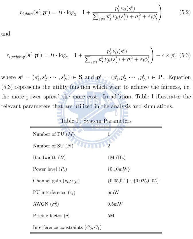
Moreover, it is noted that the immediate utility function 𝑟𝑖 are defined in two types : 𝑟𝑖,𝑑𝑎𝑡𝑎(𝒔𝑡, 𝒑𝑡) = 𝐵 ⋅ log2 1 + 𝑝 𝑡 𝑖𝜈𝑖𝑖(𝑠𝑡𝑖) ∑ 𝑗∕=𝑖𝑝𝑡𝑗𝜈𝑗𝑖(𝑠𝑗𝑡) + 𝜎𝑖2 + 𝜀𝑖𝜙𝑡𝑖 ) (5.2) and 𝑟𝑖,𝑝𝑟𝑖𝑐𝑖𝑛𝑔(𝒔𝑡, 𝒑𝑡) = 𝐵 ⋅ log2 1 + 𝑝 𝑡 𝑖𝜈𝑖𝑖(𝑠𝑡𝑖) ∑ 𝑗∕=𝑖𝑝𝑡𝑗𝜈𝑗𝑖(𝑠𝑗𝑡) + 𝜎𝑖2 + 𝜀𝑖𝜙𝑡𝑖 ) − 𝑐 × 𝑝𝑡 𝑖 (5.3) where 𝒔𝑡 = (𝑠𝑡 1, 𝑠𝑡2, ⋅ ⋅ ⋅ , 𝑠𝑡𝑁) ∈ S and 𝒑𝑡 = (𝑝𝑡1, 𝑝𝑡2, ⋅ ⋅ ⋅ , 𝑝𝑡𝑁) ∈ P. Equation
(5.3) represents the utility function which want to achieve the fairness, i.e. the more power spread the more cost. In addition, Table I illustrates the relevant parameters that are utilized in the analysis and simulations.
Table I : System Parameters
Number of PU (𝑀) 1 Number of SU (𝑁) 2 Bandwidth (𝐵) 1M (Hz) Power level (𝑃𝑖) {0,10mW} Channel gain (𝑣𝑖𝑖; 𝑣𝑗𝑖) {0.05,0.1} ; {0.025,0.05} PU interference (𝜀𝑖) 5mW AWGN (𝜎2 0) 0.5mW Pricing factor (𝑐) 5M Interference constraints (𝐶0; 𝐶1)
0 20 40 60 80 100 6.6 6.8 7 7.2 7.4 7.6 7.8 8 8.2x 10 5
Finite Time Length
Utility R 1−simulation R2−simulation R1−theoretic R 2−theoretic
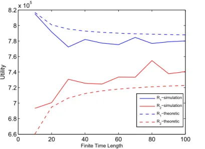
Figure 5.1: Finite Time Horizon : Time length versus expected utility under
𝐶0 = 0.5𝑚𝑊 , 𝐶1 = 0.5𝑚𝑊 and 𝑟𝑖,𝑑𝑎𝑡𝑎
5.1 Finite Time Horizon
5.1.1 Validate
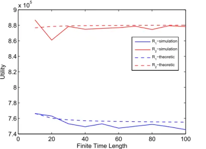
Fig.(5.1 - 5.4) and Fig () show the validations of theoretic and simulation re-sults by different utility function, 5.2 and 5.2 respectively. Because the status of expected utility doesn’t reach stable, results may have a little variation. In
addition, 𝐶0 which represents the constraint with the absence of PU mainly
affects the amount of expected utility, i.e. maximal value of expected utility
happened when 𝐶0 = 0.5𝑚𝑊 .
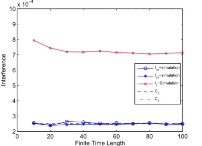
Fig.(5.5 - 5.8) and Fig () present the validations of theoretic and simula-tion interference by different utility funcsimula-tion, 5.2 and 5.2 respectively. The results show that all satisfy the interference constraint under the proposed scheme.
0 20 40 60 80 100 7.4 7.6 7.8 8 8.2 8.4 8.6 8.8 9x 10 5
Finite Time Length
Utility R1−simulation R2−simulation R 1−theoretic R 2−theoretic
Figure 5.2: Finite Time Horizon : Time length versus expected utility under
𝐶0 = 0.5𝑚𝑊 , 𝐶1 = 1𝑚𝑊 and 𝑟𝑖,𝑑𝑎𝑡𝑎 0 20 40 60 80 100 5 5.5 6 6.5 7 7.5 8x 10 5
Finite Time Length
Utility R1−simulation R2−simulation R 1−theoretic R 2−theoretic
Figure 5.3: Finite Time Horizon : Time length versus expected utility under
0 20 40 60 80 100 6.9 7 7.1 7.2 7.3 7.4 7.5x 10 5
Finite Time Length
Utility R1−simulation R 2−simulation R 1−theoretic R2−theoretic
Figure 5.4: Finite Time Horizon : Time length versus expected utility under
𝐶0 = 0.25𝑚𝑊 , 𝐶1 = 1𝑚𝑊 and 𝑟𝑖,𝑑𝑎𝑡𝑎 0 20 40 60 80 100 3 3.5 4 4.5 5 5.5x 10 −4
Finite Time Length
Interference I 02−simulation I 01−simulation I1−simulation C0 C 1
Figure 5.5: Finite Time Horizon : Time length versus expected interference
0 20 40 60 80 100 3 4 5 6 7 8 9 10 11x 10 −4
Finite Time Length
Interference I02−simulation I01−simulation I 1−Simulation C 0 C1
Figure 5.6: Finite Time Horizon : Time length versus expected interference
under 𝐶0 = 0.5𝑚𝑊 , 𝐶1 = 1𝑚𝑊 and 𝑟𝑖,𝑑𝑎𝑡𝑎 0 20 40 60 80 100 2 2.5 3 3.5 4 4.5 5 5.5x 10 −4
Finite Time Length
Interference I02−simulation I01−simulation I 1−Simulation C 0 C1
Figure 5.7: Finite Time Horizon : Time length versus expected interference
0 20 40 60 80 100 2 3 4 5 6 7 8 9 10x 10 −4
Finite Time Length
Interference I 02−simulation I01−simulation I1−Simulation C 0 C 1
Figure 5.8: Finite Time Horizon : Time length versus expected interference
under 𝐶0 = 0.25𝑚𝑊 , 𝐶1 = 1𝑚𝑊 and 𝑟𝑖,𝑑𝑎𝑡𝑎
5.1.2 Compare with greedy mechanism
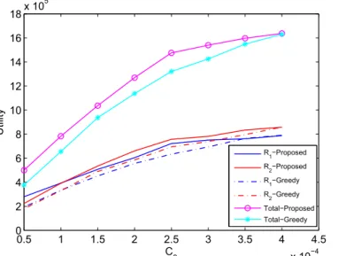
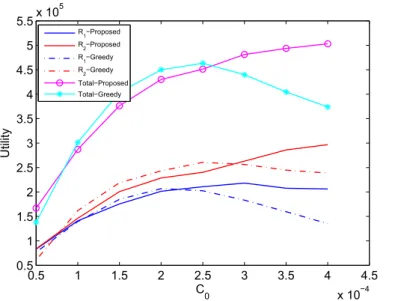
Fig.(5.9 - 5.10) display the comparison of proposed and greedy mechanisms in equation (5.2). These outcomes don’t show the advantage of proposed scheme due to the design of utility function. However, Fig.(5.11 - 5.12) show that proposed scheme have better performance than greedy one. Because of the curve of the equation (5.3), game theory has the ability to adjust the action to the maximal value. On the other hand, the greedy scheme always choose the maximum power which not the optimal decision. In addition,
we can observe the existence of optimal action when 𝐶0 ≥ 0.25𝑚𝑊 and
0.5 1 1.5 2 2.5 3 3.5 4 4.5 x 10⁻⁴ 0 2 4 6 8 10 12 14 16 18x 10 5 C 0 Utility R 1−Proposed R2−Proposed R 1−Greedy R 2−Greedy Total−Proposed Total−Greedy
Figure 5.9: Finite Time Horizon : 𝐶0 versus expected interference under
𝑟𝑖,𝑑𝑎𝑡𝑎 4.5 5 5.5 6 6.5 7 7.5 8 8.5 x 10⁻⁴ 2 4 6 8 10 12 14 16x 10 5 C 1 Utility R1−Proposed R2−Proposed R 1−Greedy R 2−Greedy Total−Proposed Total−Greedy
Figure 5.10: Finite Time Horizon : 𝐶1 versus expected interference under
0.5 1 1.5 2 2.5 3 3.5 4 4.5 x 10⁻⁴ 0.5 1 1.5 2 2.5 3 3.5 4 4.5 5 5.5x 10 5 C 0 Utility R1−Proposed R2−Proposed R1−Greedy R2−Greedy Total−Proposed Total−Greedy
Figure 5.11: Finite Time Horizon : 𝐶0 versus expected interference under
𝑟𝑖,𝑝𝑟𝑖𝑐𝑖𝑛𝑔 4.5 5 5.5 6 6.5 7 7.5 8 8.5 x 10⁻⁴ 0.5 1 1.5 2 2.5 3 3.5 4 4.5 5x 10 5 C 1 Utility R1−Proposed R2−Proposed R1−Greedy R2−Greedy Total−Proposed Total−Greedy
Figure 5.12: Finite Time Horizon : 𝐶1 versus expected interference under
0 200 400 600 800 1000 0 2 4 6 8 10 12 14x 10 5 Time Length Utility R1−simulation R 2−simulation R 1−theoretic R2−theoretic
Figure 5.13: Infinite Time Horizon : Time length versus expected utility
under 𝐶0 = 0.5𝑚𝑊 , 𝐶1 = 0.5𝑚𝑊 and 𝑟𝑖,𝑑𝑎𝑡𝑎
5.2 Infinite Time Horizon
5.2.1 Validate
Fig.(5.13 - 5.16) and Fig () show the validations of theoretic and simulation results by different utility function, equation (5.2) and (5.3) respectively. These results show that the proposed scheme can predict the expected utility when time length large enough. It noted that in Fig.(5.15) and Fig.(5.16) the expected utility have a few variation in former time slot. Due to the strict
interference constraint of 𝐶0, SUs have lower probability to transmit data
when absence of PU. So, it may need more time to converge the theoretic value of expected utility.
0 200 400 600 800 1000 5 6 7 8 9 10 11 12x 10 5 Time Length Utility R1−simulation R2−simulation R 1−theoretic R 2−theoretic
Figure 5.14: Infinite Time Horizon : Time length versus expected utility
under 𝐶0 = 0.5𝑚𝑊 , 𝐶1 = 1𝑚𝑊 and 𝑟𝑖,𝑑𝑎𝑡𝑎 0 200 400 600 800 1000 0 2 4 6 8 10x 10 5 Time Length Utility R 1−simulation R2−simulation R1−theoretic R 2−theoretic
Figure 5.15: Infinite Time Horizon : Time length versus expected utility
0 200 400 600 800 1000 5 6 7 8 9 10x 10 5 Time Length Utility R 1−simulation R 2−simulation R 1−theoretic R2−theoretic
Figure 5.16: Infinite Time Horizon : Time length versus expected utility
under 𝐶0 = 0.25𝑚𝑊 , 𝐶1 = 1𝑚𝑊 and 𝑟𝑖,𝑑𝑎𝑡𝑎 0 200 400 600 800 1000 0 1 2 3 4 5 6 7 8x 10 −4 Time Length Interference I 01−simulation I 02−simulation I1−Simulation C0 C 1
Figure 5.17: Infinite Time Horizon : Time length versus expected interference
0 200 400 600 800 1000 0 0.2 0.4 0.6 0.8 1 1.2x 10 −3 Time Length Interference I 01−simulation I 02−simulation I1−Simulation C0 C 1
Figure 5.18: Infinite Time Horizon : Time length versus expected interference
under 𝐶0 = 0.5𝑚𝑊 , 𝐶1 = 1𝑚𝑊 and 𝑟𝑖,𝑝𝑟𝑖𝑐𝑖𝑛𝑔 0 200 400 600 800 1000 0 1 2 3 4 5 6x 10 −4 Time Length Interference I01−simulation I 02−simulation I 1−Simulation C0 C1
Figure 5.19: Infinite Time Horizon : Time length versus expected interference
0 200 400 600 800 1000 0 0.2 0.4 0.6 0.8 1 1.2x 10 −3 Time Length Interference I 01−simulation I02−simulation I 1−Simulation C 0 C 1
Figure 5.20: Infinite Time Horizon : Time length versus expected interference
under 𝐶0 = 0.25𝑚𝑊 , 𝐶1 = 1𝑚𝑊 and 𝑟𝑖,𝑝𝑟𝑖𝑐𝑖𝑛𝑔
5.2.2 Compare with greedy mechanism
Fig.(5.21 - 5.24) show the comparing of proposed and greedy mechanisms in equation (5.2) and (5.3) respectively. These outcomes show that proposed scheme always better than the greedy scheme.
5.2.3 Effect of channel sensing error
Fig.(5.25 - 5.26) illustrate the effect of channel sensing error in equation (5.2) and (5.3) respectively. When error percent in equation (5.1) lower than 0.2, the expected interference doesn’t exceed the constraint. However, it will cause higher interference when error percent overstep 0.2. According to this
situation, we can set the strictly (e.g. 𝐶0 = 0.45𝑚𝑊 ) to make up the effect
0.5 1 1.5 2 2.5 3 3.5 4 4.5 x 10⁻⁴ 0 2 4 6 8 10 12 14 16 18x 10 5 C 0 Utility R1−Proposed R 2−Proposed R 1−Greedy R2−Greedy Total−Proposed Total−Greedy
Figure 5.21: Infinite Time Horizon : 𝐶0 versus expected interference under
𝑟𝑖,𝑑𝑎𝑡𝑎 4 5 6 7 8 x 10⁻⁴ 0 2 4 6 8 10 12 14 16x 10 5 C 1 Utility R1−Proposed R 2−Proposed R 1−Greedy R2−Greedy Total−Proposed Total−Greedy
Figure 5.22: Infinite Time Horizon : 𝐶1 versus expected interference under
0.5 1 1.5 2 2.5 3 3.5 4 4.5 x 10⁻⁴ 0 2 4 6 8 10 12 14 16x 10 5 C 0 Utility R 1−Proposed R 2−Proposed R1−Greedy R2−Greedy Total−Proposed Total−Greedy
Figure 5.23: Infinite Time Horizon : 𝐶0 versus expected interference under
𝑟𝑖,𝑝𝑟𝑖𝑐𝑖𝑛𝑔 4 5 6 7 8 x 10⁻⁴ 0.4 0.6 0.8 1 1.2 1.4 1.6x 10 6 C 1 Utility R 1−Proposed R2−Proposed R1−Greedy R2−Greedy Total−Proposed Total−Greedy
Figure 5.24: Infinite Time Horizon : 𝐶1 versus expected interference under
−0.42 −0.2 0 0.2 0.4 0.6 0.8 1 2.5 3 3.5 4 4.5 5 5.5x 10 −4 Error percent Interference I 01−correct I 02−correct I1−correct I01−error I 02−error I 1−error C0 C1
Figure 5.25: Infinite Time Horizon : error percent versus expected
interfer-ence under 𝑟𝑖,𝑑𝑎𝑡𝑎 −0.42 −0.2 0 0.2 0.4 0.6 0.8 1 2.5 3 3.5 4 4.5 5 5.5x 10 −4 Error percent Interference I 01−correct I 02−correct I1−correct I 01−error I 02−error I 1−error C0 C 1
Figure 5.26: Infinite Time Horizon : error percent versus expected
Chapter 6
Conclusion
This paper proposes a dynamic power management scheme for maximizing the expected utility function in the cognitive radio networks (CRN). The variations from both the spectrum holes and the channel gains are considered in the network scenarios for the CRN. Based on the Markovian property of dynamic environment, finite and infinite time horizon situations are both investigated. Associated with the constraints of allowable interferences, the constrained stochastic games are utilized to acquired the optimal policies based on the objective of maximized the exptected utility function. The existence of the constrained Nash equilibrium can be proved and is served as the optimal policies for the power management problem. Simulations are performed to validate the correctness of the optimal policies that are proposed for the dynamic power management in CRN. Moreover, the proposed schemes have better performance than greedy mechanism and channel sensing error
Bibliography
[1] M. McHenry, “Spectrum White Space Measurements,” New America Foundation Broadband Forum, 2003.
[2] G. Ganesan, Y. Li, and S. Li, “Spatiotemporal Sensing in Cognitive Radio Networks,” IEEE J.Sel.Areas Commun., vol. 26, pp. 5–12, 2008. [3] S. M. Mishra, A. Sahai, and R. W. Brodersen, “Cooperative Sensing among Cognitive Radios,” Proc.IEEE ICC, vol. 4, pp. 1658–1663, 2006. [4] F. Wang, M. Krunz, and S. Cui, “Spectrum Sharing in Cognitive Radio
Networks,” Proc.IEEE INFOCOM, pp. 1885–1893, 2008.
[5] J. Jia, Q. Zhang, and X. Shen, “A Hardware-Constrained Cognitive MAC for Efficient Spectrum Management,” IEEE J.Sel.Areas Com-mun., vol. 26, pp. 106 –117, 2008.
[6] H. Su and X. Zhang, “Cross-Layer Based Opportunistic MAC Protocols for QoSProvisionings Over Cognitive Radio Wireless Networks,” IEEE J.Sel.Areas Commun., vol. 26, pp. 118–129, 2008.