追蹤季節性時間數列模型之流程資料 - 政大學術集成

全文

(1)國立政治大學統計學系碩士學位論文. 追蹤季節性時間數列模型之流程資料 Monitoring process data with seasonal time. 治. 政 model大 series. 立. ‧. ‧ 國. 學. n. er. io. sit. y. Nat. al. C. i n U. v. h e n g楊素芬指導教授: c h i 博士鄭宗記博士研究生：. 王儀茹. 中華民國 102 年 6 月.

(2) 謝辭碩士生活經歷許多挑戰，學習許多知識以及良好的態度，讓我成長不少。在論文撰寫之時，遇到許多挫折跟難關，但關關難過關關過，論文還是順利完稿，在此謹以此文表達我的感激之情。首先，由衷感謝指導教授楊素芬教授及鄭宗記教授。謝謝楊老師這兩年嚴格的指導，讓我學習到許多品管上的知識跟待人接物的道理，讓. 政治大. 我知道做事要講求效率跟品質。也感謝鄭老師在撰寫論文時的幫助，老師. 立. 的細心指導讓我在專業知識上有極大收穫。還有，感謝口試委員葉小蓁老. ‧ 國. 學. 師、侯家鼎老師以及蕭又新老師的不吝提點，給予許多寶貴的意見，使論. ‧. Nat. y. 文更加完善，也感謝教授們在口試後的勉勵與祝福。碩士兩年，感謝同窗. er. io. sit. 的陪伴，彼此互相加油打氣，為這段生活增加不少樂趣。. n. 最後感謝我的家人，謝謝你們給予我精神上的支持跟鼓勵，使我能坦 a v. i l C n hengchi U 然面對所遭遇的一切，期盼未來自己也會勇敢面對，對自己負責。. 王儀茹謹致中華民國 102 年六月.

(3) Abstract Control charts are designed and evaluated under the assumption that the observations from the process are independent and identically distributed. However, the independence assumption is often violated in practice. Autocorrelation may be represented in many processes. To solve this problem, it is becoming more common to obtain profiles at each time period. Profile monitoring is the use of control charts for cases in which the quality of a process or product can be characterized by a functional relationship between a response. 政治大 model, we propose several monitoring approaches to detect the out-of-control profiles. After 立 variable and one or more explanatory variables. For the data with seasonal time series. ‧. ‧ 國. io. sit. y. Nat. n. al. er. results.. 學. considering both Phase I and Phase II schemes, a real example is given to illustrate the. Ch. engchi. i n U. v.

(4) Contents Chapter 1. Introduction ............................................................................... 1. Chapter 2. Research Methods ..................................................................... 4. 2.1. Control Bands under each time unit .........................................................................5. 2.1.1 Introduction ..........................................................................................................5 2.1.2 Model assumptions and notations ........................................................................5. 政治大 Introduction ..........................................................................................................7 立. 2.2 2.2.1. Confidence bands based on Kalman Filter approach ...............................................7. ‧ 國. 學. 2.2.2 Model assumption and notation............................................................................8 2.2.3 State Space Model ..............................................................................................10. ‧. 2.2.4 Kalman Filter ......................................................................................................12. Nat. y. Confidence Bands based on Bootstrap approach ...................................................15. sit. 2.3. n. al. er. io. 2.3.1 Introduction ........................................................................................................15. i n U. v. 2.3.2 Bootstrap Procedure ...........................................................................................16 2.3.3 2.4. Ch. engchi. Control chart for monitoring variance of the residuals.......................................16 Hotelling T2 control charts .....................................................................................17. 2.4.1 Introduction ........................................................................................................17 2.4.2 Hotelling’s T2 Control Chart...............................................................................17 2.4.3 T2 chart for monitoring coefficients of a profile.................................................18 2.4.4 T2 chart for monitoring variance of the residuals ...............................................19. Chapter 3. Real data analysis: Power Consumption in National. Chengchi University ........................................................................................ 21.

(5) 3.1. Introduction ............................................................................................................21. 3.2. Data classification...................................................................................................22. 3.3. Phase I and Phase II control scheme ......................................................................30. 3.3.1 Model assumption and identification .................................................................30 3.3.2 Phase I and Phase II control charts .....................................................................35 3.3.3 Example of Semester without AC data (WOAC data) .......................................36 3.3.4 Example of Semester with AC data (WAC data) ................................................44. 政治大. Performance Comparison .......................................................................................52. Chapter 4. 立. Conclusions .............................................................................. 61. 學. ‧ 國. 3.4. References ........................................................................................................ 62. ‧. n. er. io. sit. y. Nat. al. Ch. engchi. i n U. v.

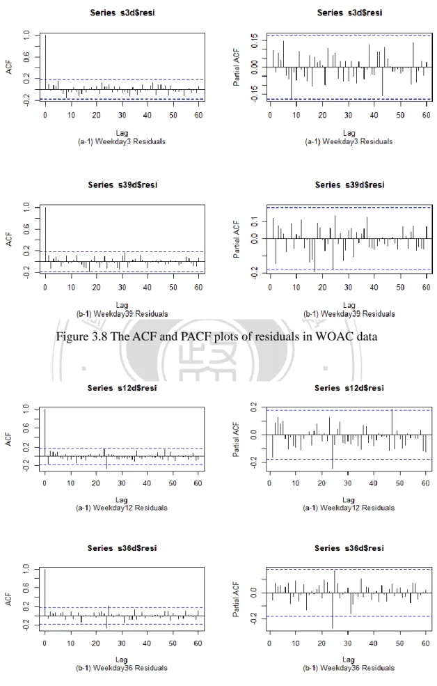
(6) Figure 3.1 Plot of Electricity Monitor System .......................................................................21 Figure 3.2 Plot of the electricity consumption and corresponding temperature in March and June ........................................................................................................................22 Figure 3.3 Plot of power and corresponding temperature for NE data in WOAC data ..........26 Figure 3.4 Plot of power and corresponding temperature for SE data in WOAC data ..........27 Figure 3.5 Plot of power and corresponding temperature for NE data in WAC data .............28 Figure 3.6 Plot of power and corresponding temperature for SE data in WAC data..............29 Figure 3.7 Plot of the electricity consumption .......................................................................30. 政治大. Figure 3.8 The ACF and PACF plots of residuals in WOAC data .........................................34. 立. Figure 3.9 The ACF and PACF plots of residuals in WAC data .............................................34. ‧ 國. 學. Figure 3.10 Plot of control bands under each hour in Phase I for WOAC data .....................37 Figure 3.11 Plot of CB based on Kalman Filter approach in Phase I for WOAC data ..........39. ‧. Figure 3.12 Plot of CB based on Bootstrap approach in Phase I in WOAC data ...................40. Nat. sit. y. Figure 3.13 Plot of standard deviation of the residuals in WOAC data .................................41. n. al. er. io. Figure 3.14 Plot of the values of T2 statistic for each weekday in Phase I for WOAC data ..43. i n U. v. Figure 3.15 Plot of the values of T2 statistic for Special-Event Weekdays Data for WOAC data. Ch. engchi. ................................................................................................................................43 Figure 3.16 Plot of control bands under each hour in Phase I for WAC data .........................45 Figure 3.17 Plot of CB based on Kalman Filter approach in Phase I for WAC data ..............47 Figure 3.18 Plot of CB based on Bootstrap approach in Phase I for WAC data ....................48 Figure 3.19 Plot of standard deviation of the residuals for WAC data ...................................49 Figure 3.20 Plot of the values of T2 statistic for each weekday in Phase I for WAC data......51 Figure 3.21 Plot of the values of T2 statistic for SE data for WAC data .................................51 Figure 3.22 Plot of CB for weekday 6 under out-of-control for WOAC ...............................55.

(7) Figure 3.23 Plot of CB for weekday8 under out-of-control for WOAC ................................56 Figure 3.24 Plot of CB for weekday46 under out-of-control for WOAC ..............................57 Figure 3.25 Plot of CB for weekday15 under out-of-control for WAC ..................................58 Figure 3.26 Plot of CB for weekday31 under out-of-control for WAC ..................................59 Figure 3.27 Plot of CB for weekday33 under out-of-control for WAC ..................................60. Table 2.1 Data Structure ...........................................................................................................8 Table 3.1 The grouping table ................................................................................................24. 政治大. Table 3.2 Parameter Estimation of SARMA model for NE data in WOAC dataset ..............32. 立. Table 3.3 Parameter Estimation of SARMA model for SE data in WOAC dataset ...............32. ‧ 國. 學. Table 3.4 Parameter Estimation of SARMA model for NE data in WAC dataset ..................33. ‧. Table 3.5 Parameter Estimation of SARMA model for SE data in WAC dataset ..................33 Table 3.6 Table of special event .............................................................................................35. y. Nat. io. sit. Table 3.7 Table of the OCC time point by control bands under each hour for WOAC data ..37. n. al. er. Table 3.8 Table of the OOC time point by CB based on Kalman Filter approach for WOAC39. Ch. i n U. v. Table 3.9 Table of the OOC time point by CB based on Bootstrap approach for WOAC .....40. engchi. Table 3.10 Table of the best time series model in Weekday1,6,9 for WOAC data ................42 Table 3.11 Table of the OOC time point by control bands under each hour for WAC ...........45 Table 3.12 Table of the OOC time point by CB based on Kalman Filter approach for WAC 47 Table 3.13 Table of the OOC time point by CB based on Boostrap approach for WAC........48 Table 3.14 Table of best time series model in Weekday14, 31, 33, 35 for WAC data .........50 Table 3.15 Comparison Table for SE data in WOAC data .....................................................54 Table 3.16 Comparison Table for SE data in WAC data ........................................................54.

(8) Chapter 1 Introduction The statistical control chart is a useful tool to monitor processes with the objectives of analyzing the quality problem and improving process quality. When unusual sources of variability are present, it signals. In any production process, a certain amount of inherent or natural variability will always exist. Common cause is said to be in statistical control, while special causes is said to be an out-of-control process. The former comes from natural random variability, the latter arises from machines, operators, or raw materials. If a process. 治政大of control so that we can the control chart, it can tell whether the process is in or out 立. has only random causes, it is said to be in-control, or it is said to be out-of-control. By using. perform correct actions to let the process back into control when it is necessary. The. ‧ 國. 學. statistical properties of control charts have traditionally been evaluated under the. ‧. assumption that observations from the process at different times are independent random. sit. y. Nat. variables. However, the observations from many processes exhibit autocorrelation that may. io. er. be the result of dynamics that are inherent to the process. Autocorrelation is more likely to be observed in processes when observations are closely spaced in time. To solve this. al. n. v i n problem, due to advances in technology, C h it is becomingUmore common to obtain profiles at engchi each time period. Profile monitoring is the use of control charts for cases in which the. quality of a process or product can be characterized by a functional relationship between a response variable and one or more explanatory variables. In these cases a control strategy should be able to signal rapidly with an alarm if the profile is different from the in-control profile. Many authors have recently investigated issues related to profile monitoring. Kang and Albin (2000) and Kim et al. (2003) introduced methods to monitor simple linear profiles. Zou et al.(2008) and Mahmoud et al.(2007) considered change point methods in profile monitoring. Kazemzade et al.(2008) studied polynomial profiles. Zou et al.(2008) 1.

(9) combined multivariate exponentially weighted moving average procedure with a generalized likelihood ratio test based on nonparametric regression to monitor nonlinear profiles. Also nonlinear profiles monitoring was discussed by researchers including Ding et al.(2006), Moguerza et al.(2007), Williams et al.(2007), and Vaghefi et al.(2009), Noorossana et al.(2010), Zou et al.(2012) proposed methods to monitor multivariate linear profiles. Noorossana et al.(2011) showed the effect of non–normality on the monitoring of simple linear profiles. Several authors including Jensen et al.(2008), Noorossana et al.(2008), Soleimani et al. (2009) and, Kazemzadeh et al.(2010) addressed issues related to. 治政大profile autocorrelation in (2011) proposed methods to consider within and between 立. autocorrelation in linear, non-linear, and polynomial profiles. Soleimani and Noorossana. multivariate linear profiles in phase II. These monitoring procedures suppose that is more. ‧ 國. 學. efficient to summarize the in-control performance with a parametric model and monitor for. ‧. shifts in the model parameters. Cheng and Yang (2013) consider a multiple linear regression. y. Nat. with random errors following an autoregressive moving-average (ARMA) model. They. er. io. sit. used a Hotelling T2 control chart to monitor the coefficients of the model and a Hotelling T2 control chart to monitor the variance of residuals with time. However, for the data with. al. n. v i n seasonal time series model, it hasC been rarely discussed. In this paper, we propose several hengchi U. approaches to detect this kind of data. The aim of this paper is to construct confidence bands and control charts based on different approaches for the data with seasonal autoregressive moving average model (SARMA) to monitor the out-of-control profiles. If a profile or a monitoring statistic falls in the confidence bands or control limits we established, then it is in-control profile, while a profile performs differently from the in-control profile that we determined, it can be identified to be out-of-control. We propose a practical guide for monitoring profiles. Furthermore, the numerical results from a real application show our proposed methods are effective in detecting out-of-control profiles. Based on the observed 2.

(10) in-control profiles we wish to establish an adequate confidence bands and control charts for the underlying functional relationship. Then this confidence bands can serve as a control chart for phase II process monitoring. This is organized as follows. Chapter 2 represents four monitoring methods for the data with seasonal time series model. Chapter 3 gives a real data example, which originally inspired this paper. Chapter 4 draws conclusions and provides direction for future work.. 立. 政治大. ‧. ‧ 國. 學. n. er. io. sit. y. Nat. al. Ch. engchi. 3. i n U. v.

(11) Chapter 2. Research Methods. Control charts (Shewhart, CUSUM, EWMA) are designed and evaluated under the assumption that the observations from the process are independent and identically distributed. However, the independence assumption is often violated in practice. Autocorrelation may be represented in many processes such as chemical process where consecutive measurements on process are highly correlated. If we use the traditional control charts and run rules to monitor the correlated data, because of the violation of the independence, many observations may be identified to be out-of-control. In this study, we present four monitoring methods for. 政治大. the process that deal with correlated data, especially date having the periodical behavior.. 立. Many time series contain a seasonal phenomenon that repeats itself after a regular period of. ‧ 國. 學. time. Seasonal phenomena may stem from factor such as weather, or customs. For example, the consumption of the electricity is higher in summer but lower in winter. To deal with these. ‧. types of data, we mainly use a more sophisticated method based on time series model, like. y. Nat. sit. seasonal ARMA model. Using the in-control SARMA model to construct the control bands,. n. al. er. io. confidence bands and control charts based on four different methods to monitor the. i n U. v. out-of-control time series model. The out-of-control detect performance of the bands based. Ch. engchi. on four different methods are compared.. 4.

(12) 2.1 Control Bands under each time unit 2.1.1. Introduction. Control chart limits are usually established on the assumption that there is no serial correlation within the samples and data are from normal populations. If the observations are correlated, the traditional control limits for the shewhart control chart need to be revised. Here is a simple idea that we just want to find out the outliers at time t by using the three-sigma method that determine the outliers. Different from the conception of the shewhart control chart, because the means and variances of the process vary with time, we. 政治大 variance 𝜎 . We will explain how to construct the control bands under each time unit below. 立. assume that at time t the observation which is sampled from a process with mean 𝜇𝑡 and 2 𝑡. ‧ 國. 學. 2.1.2. Model assumptions and notations. ‧. The properties of control charts are usually calculated under the assumption that the observations are independent normal random variables with constant mean and variance. This. y. Nat. n. Ch. er. io. al. 𝑋𝑡 = 𝜇 + 𝜀𝑡 , 𝑡 = 1,2, , … , 𝑇. sit. implies that 𝑋𝑡 can be written as. i n U. v. (2.1). where 𝜇 is the process mean. It is also assumed that the process mean 𝜇 is constant at a. engchi. target value when the process is in-control and can change to some other value when a special cause occurs. Suppose 𝜇 and σ are both known. Then the upper control limit and lower control limit for the X chart are 𝑈𝐶𝐿 = 𝜇 + 3 × 𝜎 ,. (2.2). 𝐿𝐶𝐿 = 𝜇 − 3 × 𝜎 .. (2.3). To the model observations from an autocorrelated process, if the control limits are (2.2), (2.3) 5.

(13) which are constant, it can’t show the different control limits at each time. When the independence assumption is violated (even at the low levels of correlation over time), the control charts do not perform well. Typically, these control charts will give much higher false alarm rates than when the data is uncorrelated over time. So we construct the control bands under each time unit. We suppose that 𝑥𝑡𝑖 from subgroup i at time t, is assumed to satisfy 𝑥𝑡𝑖 = 𝜇𝑡 + 𝜀𝑡𝑖 , i=1,2,…,N, t=1,2,3,…,T. (2.4). where 𝜀𝑡𝑖 are random variables with mean zero and variance 𝜎𝑡2 . The interpretation of 𝜇𝑡 is. 治政大 be are known, the confidence bands will 立. the random process mean at time t . Suppose 𝜇𝑡 and. 𝜎𝑡2 .. (2.5). 學. ‧ 國. 𝑈𝐶𝐿 = 𝜇𝑡 + 3 × 𝜎𝑡 , 𝐿𝐶𝐿 = 𝜇𝑡 − 3 × 𝜎𝑡 .. (2.6). ‧. If 𝜇𝑡 and 𝜎𝑡2 are unknown, we use the estimators to construct the control bands. The. io. 𝑥̅ 𝑡 = ∑ 𝑖=1. n. al. and. Ch. y. sit. 𝑁. 𝑥𝑡𝑖 , 𝑁. engchi. er. Nat. estimated sample mean and standard deviation in the model (2.4) are. i n U. v. 2 ∑𝑁 𝑖=1(𝑥𝑡𝑖 − 𝑥̅𝑡 ) √ 𝑠𝑡 = . 𝑁−1. By the idea of outlier detection, we construct the control bands with mean ±3 times standard deviation at time t by the empirical rule, so the control bands will be 𝑈𝐶𝐵𝑡1_1 = 𝑥̅𝑡 + 3 × 𝑠𝑡 ,. (2.7). 𝐿𝐶𝐵𝑡1_1 = 𝑥̅𝑡 − 3 × 𝑠𝑡 .. (2.8). Plot the observation 𝑥𝑡𝑖 from subgroup i , i=1, 2,…,N, into (2.7) and (2.8) and check whether 𝑥𝑡𝑖 is in-control. When all the 𝑥𝑡𝑖 fall in the control bands, we can use the control 6.

(14) bands to detect the out-of-control mean. If 𝑥𝑡𝑖 falls outside the control bands, it is identified to be out-of-control. For monitoring the process variability, we use the moving standard deviation (MS) for each subgroup to establish the control bands of MS under each time unit. We calculate the standard deviation of two observation at time t-1 and t for subgroup i as moving standard deviation, which is denoted as 𝑀𝑆𝑡𝑖 , t=2, 3, … , T, i =1, 2, …, N, and the control bands of MS under each time unit will be ̅̅̅̅𝑡 + 3 × 𝑠𝑀𝑆 , 𝑈𝐶𝐵𝑡1_2 = 𝑀𝑆 𝑡 𝑁. (2.9). 政治大 from 立subgroup i , i=1, 2,…,N, into (2.9) and check whether 𝑀𝑆 𝑁. ̅̅̅̅̅. ̅̅̅̅𝑡 = ∑𝑖=1 𝑀𝑆𝑡𝑖 , and 𝑠𝑀𝑆 = √∑𝑖=1(𝑀𝑆𝑡𝑖 −𝑀𝑆𝑡), t=2, 3,.., T, i=1,2,…,N. Plot the moving where 𝑀𝑆 𝑡 𝑁 𝑁−1 standard deviation 𝑀𝑆𝑡𝑖. 𝑡𝑖. is. ‧ 國. 學. in-control. When all the 𝑀𝑆𝑡𝑖 fall in the control bands, we can use the control bands to detect the out-of-control data. If 𝑀𝑆𝑡𝑖 falls outside the control bands, it is identified to be. ‧. out-of-control.. sit. y. Nat. We use these two control bands simultaneously to monitor our data, so if one of the. n. al. er. io. charts detects the points that exceed the upper bands, the subgroup may be identified to be. v. out-of-control. We then need to find the cause of out-of-control which makes the subgroup to be out-of-control.. Ch. engchi. i n U. 2.2 Confidence bands based on Kalman Filter approach 2.2.1. Introduction. In many applications the quality of a process or product is the best characterized and summarized by a functional relationship between a response variable and one or more explanatory variables instead of by the distribution of a single quality characteristic. Due to advances in technology, profile monitoring is used to understand and to check the stability of this relationship over time. At each sampling stage one observes a collection of data 7.

(15) points that can be represented by a curve (profile). In many cases of profile monitoring, it is efficient to summarize the in-control shape of the profile with parametric model and monitor for shifts in the parameters of this model. The confidence bands are based on the estimated parameters of the model from successive profile data observed over time. In section 2.1, we don’t consider the problem of correlated data, and just construct the confidence bands for each time unit. Here we use the model-based method. An approach that has proved useful in dealing with autocorrelated data is time series model. We try to find an underlying in-control profile and use two approaches to build its confidence bands,. 治政 confidence bands, it is in-control. But if one of the fitted大 values of a profile exceeds the 立. one is Kalman Filter approach, the other is bootstrap approach. If a profile fall inside the. confidence bands, it is identified to be an out-of-control profile. We first introduce the. ‧ 國. 學. confidence bands based on Kalman Filter approach.. ‧. 2.2.2. Model assumption and notation. y. Nat. sit. Suppose there are N subgroups in a group, which can be expressed as “ith subgroup ”,. n. al. er. io. i=1,2,…,N. We tabulate the data as follows and each row in the table can be viewed as a realization of a time series.. Ch. engchi. i n U. v. Table 2.1 Data Structure. Subgroup(i)/ time(t). 1. ⋯. T. 1. 𝑥11. ⋯. 𝑥𝑡1. ⋮. ⋮. ⋮. ⋮. N. 𝑥1𝑁. ⋯. 𝑥𝑇𝑁. Box and Jenkins (1976), who have been the main contributors to making the ARMA models popular, have proposed a class of models for describing a time series with periodical behavior. 8.

(16) Assume 𝑥𝑡𝑖 is the observed variable at time t, follows an SARMA process, which can be expressed as: 𝜑𝑝 (𝐵)𝜙𝑃 (𝐵 𝑠 )𝑥𝑡 = 𝑐 + 𝜃𝑞 (𝐵)𝛩𝑄 (𝐵 𝑠 )𝑎𝑡 , 𝑎𝑡. 𝑖. 𝑖. 𝑑 𝑊𝑁(0, 𝜎𝑎2 ) ~. (2.10). 𝑡 = 1,2, . . , 𝑇 where 𝑎𝑡 is white noise 𝜑𝑝 (𝐵) = 1 − 𝜑1 𝐵 − ⋯ − 𝜑𝑝 𝐵 𝑝 𝛷𝑃 (𝐵 𝑠 ) = 1 − 𝛷1 𝐵 − ⋯ − 𝛷𝑃 𝐵𝑃𝑆. 政治大立𝛩 (𝐵) = 1 − 𝛩 𝐵 − ⋯ − 𝛩 𝐵. 𝜃𝑞 (𝐵) = 1 − 𝜃1 𝐵 − ⋯ − 𝜃𝑞 𝐵 𝑞 𝑄. 1. 𝑄. 𝑄𝑆. ‧ 國. 學. B is the backward shift operator. It means the same SARMA(p, q)×(P,Q)s model is assumed to apply to each subgroup.. ‧. In the model-based methods, we use time series model to fit our series data. Our. sit. y. Nat. purpose is to build the confidence bands of the fitted values, which is denoted as 𝑥̂𝑡𝑖 ,. n. al. er. io. t=1,2,…,T, i=1,2,…,N. After constructing the confidence bands, we use the confidence. v. bands to detect the out-of-control profiles. Due to the difficulty of computing the variance. Ch. engchi. i n U. of 𝑥̂𝑡𝑖 , we can’t derive it directly by a simple equation. However, if we use the function “fitted” in R, we can only get the point estimators of 𝑥𝑡𝑖 and we don’t have the variance of 𝑥̂𝑡𝑖 , which can be expressed as 𝑣𝑎𝑟(𝑥̂𝑡𝑖 ). The problem becomes how to estimate the variance of the fitted values to build the confidence bands. Because the function ”fitted” in R does not give 𝑣𝑎𝑟(𝑥̂𝑡𝑖 ), we use the Kalman Filter approach to build the confidence bands with state-space equations. Kalman Filter is a set of recursion equations for determining the optimal estimates of the state vector given information available at time t. The following introduce the general state space model and put common time series models into state space form, summarize the main algorithm used for the analysis of the state space models, and 9.

(17) illustrate how to construct the confidence bands using the in-control data.. 2.2.3. State Space Model. The state-space model (sometimes called the dynamic model) was originally developed by Kalman(1960) and Kalman and Bucy (1961) for control of linear systems and has more recently become widely used for the analysis of time series data. We assume that a model concerns a series of vector 𝛼𝑡 , which are called “state vectors”. These state variable will typically not be observed and the other main ingredient is therefore the observed variables 𝑌𝑡 . First step to construct the confidence bands is to write the model in state space form. A. 政治大. state space model consists of two equations. State equation describes the evolution of the. 立. system, and observation equation describes the relation between the state of the system and. ‧ 國. 學. the observations. The two equations can be written below.. ‧. I.. State Equation. y. Nat. sit. The state equation is a VAR(1) type expression giving the rule by which v×1 random vector. n. al. er. io. 𝛼𝑡 is generated from 𝛼𝑡−1 for time points t=1,2,…,T. Specifically, the state equation is given by. Ch. engchi. i n U. 𝛼𝑡 = 𝛷𝛼𝑡−1 + 𝐺𝑉𝑡. where (a) 𝛼𝑡 is a v× 1 state vector ,t=1,2,….,T (b) 𝛷 is an v× v matrix (c) G is a v× 1 matrix (d) 𝑉𝑡 ~MVN(0,Q) is multivariate normal white noise (e) The process is initialed with a vector 𝛼0 ~𝑁(𝜇0 , 𝑃0 ). 10. v. (2.11).

(18) II. Observation Equation The assumption in state-space analysis is that observations are made on 𝑌𝑡 which is related to 𝛼𝑡 via the observation equation. 𝑌𝑡 = 𝐴𝛼𝑡 + 𝑊𝑡. (2.12). where (a) 𝑌𝑡 is the observed time series, w× 1 vector (w can be equal to, larger than, or smaller than v) (b) A is a w× v measurement or observation matrix (c) 𝑊𝑡 ~MVN(0,R) is multivariate normal white noise. 治政大uncorrelated, and 𝛼 In equations (2.11) and (2.12), noise terms 𝑊 and 𝑉 are 立 𝑡. 𝑡. 0. is. uncorrelated with 𝑊𝑡 and 𝑉𝑡 .. ‧ 國. 學. Goal of State-Space Modeling. ‧. . y. Nat. Given a state-space model, the fundamental goal is to estimate the underlying unobserved. io. sit. signal 𝛼𝑡 given the observation Y1, Y2,…, YT for some time T. The typical procedure used to. er. accomplish this goal is to estimate the parameters (𝜇0 , 𝑃0 , 𝛷, 𝐴, 𝐺, 𝑄) of the state-space model.. al. n. v i n Use the estimated model to find the estimate of 𝛼𝑡 (for some t) in the mean square C best h elinear ngchi U sense. Specifically, we want to find E(𝛼 |Y , Y ,…, Y ). For simplicity, we will use 𝛼 to 𝑡. 1. 2. T. 𝑡|𝑇. denote E(𝛼𝑡 |Y1, Y2,…, YT) ,and we denote the mean square error by 𝑃𝑡|𝑇 = 𝐸 [(𝛼𝑡 − ′. 𝛼𝑡|𝑇 )(𝛼𝑡 − 𝛼𝑡|𝑇 ) ]. . State-Space Formulation of ARMA. ARMA processes can be written in the state-space form. In the case of a general ARMA process, one can use several representations; but the most compact one is the following (Harvey,1993,Section 4.4). Assume that given the ARMA process (with zero mean) : 11.

(19) 𝜑𝑝 (𝐵)𝑌𝑡 = 𝜃𝑞 (𝐵)𝑎𝑡 , 𝑎𝑡 ~𝑁(0, 𝜎𝑎2 ) The process can be represented in the following state space form : State:𝛼𝑡 = 𝛷𝛼𝑡−1 + 𝐺𝑉𝑡 Observation: 𝑍𝑡 = 𝐴𝛼𝑡 for t=1,2,3,…T, and time invariant system matrices. Φ=. φ1 φ2 ⋮ φv−1 [ φv. 1 0 ⋮ 0 0 0. 0 1. 0 … 0 0 1 ⋱. 0. 0 …. 0 0 ⋮ 0 1 0]. 1 θ1 G= ⋮ θv−1 [ θv ]. A = (1. 0 0 ⋯ 0). 治政 where v=max(p,q+1). The state vector 𝛼 has the form 大立 𝑧 𝑡. 𝑡. ‧. ‧ 國. 學. 𝜑2 𝑧𝑡−1 + ⋯ + 𝜑𝑝 𝑧𝑡−𝑣+1 + 𝜃1 𝑎𝑡 + ⋯ + 𝜃𝑣−1 𝑎𝑡−𝑣+2 𝛼𝑡 = 𝜑3 𝑧𝑡−1 + ⋯ + 𝜑𝑝 𝑧𝑡−𝑣+2 + 𝜃2 𝑎𝑡 + ⋯ + 𝜃𝑣−1 𝑎𝑡−𝑣+3 ⋮ 𝜑𝑣 𝑧𝑡−1 + 𝜃𝑣−1 𝑎𝑡 [ ] Dynamic linear model (DLM), however, adds an additional component to the model in. Nat. sit. y. assuming we do not observe the state vector 𝛼𝑡 directly, but can only observe a linear. n. al. er. io. transformed version of it with noise 𝑊𝑡 added as equation (2.12). In our case, we assume. i n U. v. that the observational noise is existed, and say the signal 𝛼𝑡 satisfies an SARMA(p,. Ch. engchi. q)× (P,Q)s model, so the state-space equations can be written as (2.11) and (2.12).. 2.2.4. Kalman Filter. Kalman filter is a very useful iterative procedure for obtaining the estimates 𝛼̂𝑡|𝑇 in the state-space model. The purpose is to make inference about unobservable given the observations. The main idea is that we like to estimate a state of some sort and its uncertainty. However, we do not directly observe these states. We only observed some measurements. The question now becomes, how can we still optimally use our measurements to estimate the unobserved (hidden) states and their uncertainties. Here we 12.

(20) use R package “astsa” to carry out the Kalman filter approach. Refer to the book by Shumway (1988), the Kalman Filter can be expressed as follows. Let 𝛼𝑡|𝑠 =E(𝛼𝑡 |𝑌𝑠 )=optimal estimator of 𝛼𝑡 based on 𝑌𝑠 , ′. 𝑃𝑡|𝑠 = 𝐸 [(𝛼𝑡 − 𝛼𝑡|𝑠 )(𝛼𝑡 − 𝛼𝑡|𝑠 ) |𝑌𝑠 ].. . Prediction Equations. The following equations provide one-step ahead prediction, 𝛼̂𝑡|𝑡−1 . Specifically, we observed Y1, Y2,…, Yt-1 and want to use this information to predict 𝛼𝑡 . The Kalman recursion is as follows:. 政治大 = 𝛷𝑃 𝛷 + 𝑄.. 𝛼̂𝑡|𝑡−1 = 𝛷𝛼̂𝑡−1|𝑡−1, 𝑡−1|𝑡−1. ′. ‧ 國. Filtering Equations. 學. . 立. 𝑃𝑡|𝑡−1. The filtering and prediction recursions are run simultaneously. The equations in the Kalman. io. y. sit. 𝑃𝑡|𝑡 = [𝐼 − 𝐾𝑡 𝐴𝑡 ]𝑃𝑡|𝑡−1 ,. er. Nat. 𝛼̂𝑡|𝑡 = 𝛼̂𝑡|𝑡−1 + 𝐾𝑡 (𝑌𝑡 − 𝐴𝛼̂𝑡|𝑡−1 ),. ‧. recursions for filtering, i.e., for estimating 𝛼𝑡 based on Y1,…, Yt are given by. where 𝐾𝑡 = 𝑃𝑡|𝑡−1 𝐴′ [𝐴𝑃𝑡|𝑡−1 𝐴′ + 𝑅]−1, is called the Kalman gain.. n. al. . Ch. Smoothing Equations. engchi. i n U. v. We observe value of Y1, Y2,…, YT and the goal is to estimate 𝛼𝑡 where t<T. The recursion proceeds by calculating 𝛼̂𝑡|𝑡 , 𝛼̂𝑡|𝑡−1, 𝑃𝑡|𝑡 and 𝑃𝑡|𝑡−1 ,t=1,2,…,T using the prediction and filtering equation. Then for t=T,T-1,…we calculate 𝛼̂𝑡−1|𝑇 = 𝛼̂𝑡−1|𝑡−1 + 𝐽𝑡−1 (𝛼̂𝑡|𝑇 − 𝛼̂𝑡|𝑡−1 ), 𝑃𝑡−1|𝑇 = 𝑃𝑡−1|𝑡−1 + 𝐽𝑡−1 [𝑃𝑡|𝑇 − 𝑃𝑡|𝑡−1 ]𝐽𝑡−1 ′ , where 𝐽𝑡−1 = 𝑃𝑡−1|𝑡−1 𝛷′ [𝑃𝑡|𝑡−1 ]−1 . 13.

(21) . Initialization. In order to apply the Kalman filter one has to choose a set of starting values. The most natural choice is the unconditional mean and variance. The unconditional distribution of the initial state vector 𝛼0 is therefore given by 𝛼0 ~𝑁(𝜇0 , 𝑃0 ) If the state space model is covariance stationary, then the state vector 𝛼𝑡 is covariance stationary. By Durbin and Koopman (2001), the unconditional mean of 𝛼0 , 𝜇0 =0. 𝑃0 = 𝑣𝑎𝑟(𝛼𝑡 ) = 𝑣𝑎𝑟(𝛷𝛼𝑡−1 + 𝐺𝑉𝑡 ) = 𝛷𝛴0 𝛷′ + 𝐺𝑄𝐺 ′ Then, using 𝑣𝑒𝑐(𝐴𝐵𝐶) = 𝐶 ′ ⨂𝐴 𝑣𝑒𝑐(𝐵) ,where vec is the column stacking operator,. 政治大. 𝑣𝑒𝑐(𝑃0 ) = 𝑣𝑒𝑐(𝛷𝑃0 𝛷′ ) + 𝑣𝑒𝑐(𝐺𝑄𝐺 ′ ) = (𝛷⨂𝛷)𝑣𝑒𝑐(𝑃0 ) + 𝑣𝑒𝑐(𝐺𝑄𝐺 ′ ). 立. which implies that. ‧ 國. 學. 𝑣𝑒𝑐(𝑃0 ) = (𝐼𝑣2 − 𝛷⨂𝛷)−1 𝑣𝑒𝑐(𝐺𝑄𝐺 ′ ). … 𝑡1𝑣 𝛷 … 𝑡2𝑣 𝛷 ] and 𝑡𝑖𝑗 is the element of T occupying line i and … ⋮ … 𝑡𝑣𝑣 𝛷. y. ‧. Nat. 𝑡11 𝛷 𝑡 𝛷 where 𝛷⨂𝛷 = [ 21 ⋮ 𝑡𝑣1 𝛷. n. al. er. io. v matrix 𝑃0 .. sit. column j. Here 𝑣𝑒𝑐(𝑃0 ) is an v2× 1 column vector. It can be easily reshaped to form the v×. i n U. v. Our purpose is to find the state variables 𝛼̂𝑡𝑖|𝑇 given {𝑥1𝑖 , … , 𝑥𝑇𝑖 } ,i=1,2,…,N, in. Ch. engchi. order to construct the confidence bands .The steps are as follow. . Model Identification and Building. . Form the State-Space equations. . Select initial values for the parameter{𝝁𝟎𝒊 , 𝑷𝟎𝒊 , 𝑸𝒊 , 𝑹𝒊 }. . ̂ 𝒕𝒊|𝑻 by Kalman Filter ̂ 𝒕𝒊|𝑻 and 𝑷 Estimate the state variable 𝜶. . ̂ 𝒕|𝑻 Calculate the overall confidence bands of 𝜶. For each subgroup, we calculate the confidence bands= (𝛼̂𝑡𝑖|𝑇 ∓ 𝑍 × 𝑃̂𝑡𝑖|𝑇 ),where 𝑍 = 𝑍1− 𝛼. 2𝑚. by bonferroni correction. (If we are forming m confidence intervals, and wish to have overall 14.

(22) 𝛼. confidence level of 1-α, then adjusting each individual confidence bands to the level of 1 − 𝑚 will be the analog confidence interval correction.) Then we construct the new confidence bands, which can be expressed as 𝑈𝐶𝐵𝑡2 = 𝑚𝑎𝑥(𝛼̂𝑡𝑖|𝑇 + 𝑍 ∗ 𝑃̂𝑡𝑖|𝑇 ). (2.13). 𝐿𝐶𝐵𝑡2 = 𝑚𝑖𝑛(𝛼̂𝑡𝑖|𝑇 − 𝑍 ∗ 𝑃̂𝑡𝑖|𝑇 ). (2.14). which is the widest confidence bands of the state variable 𝛼̂𝑡|𝑇 . Plot the fitted data 𝛼̂𝑡𝑖|𝑇 of subgroup i into (2.13) and (2.14) and check whether the 𝛼̂𝑡𝑖|𝑇 is in-control. If all the fitted values of a profile fall inside the bands, it is in-control. But if one of the fitted values of a. 政治大. profile exceeds the confidence bands, it is identified to be an out-of-control profile.. 立based on Bootstrap approach 2.3 Confidence Bands. ‧ 國. 學. 2.3.1. Introduction. Different from Kalman Filter method, we use the bootstrap approach to construct the. ‧. confidence bands of the fitted values instead of computing the variance of the fitted values.. Nat. sit. y. Because the computation of the variance is complicated, here is a simple way to construct the. n. al. er. io. bands. Suppose we have N subgroups (N is smaller than 10) in a dataset, so at time t there are. i n U. v. N observations. The sample size (N<30) is small and the distribution of the fitted values is. Ch. engchi. unknown, so we use the bootstrap approach. Our purpose is to make the bands for the fitted value as the confidence bands. The following explains how to construct confidence bands based on bootstrap approach. First, we fit a seasonal time series model to our observations, and the residuals follows the normal distribution with mean zero and variance 𝜎𝑎2 . Second, we bootstrap the samples 2000 times from the fitted values of response variable which follow the distribution of residuals. Third, under the fixed time unit, we build a confidence bands by taking the empirical quantiles of the 2000 fitted values we bootstrap. Finally, we use the confidence bands to detect the out-of-control profiles. 15.

(23) 2.3.2. Bootstrap Procedure. For model (2.10), after model fitting, by using the function fitted in R, we can get the fitted 2 , denoted value of 𝑥𝑡𝑖 , denoted by 𝑥̂𝑡𝑖 . By the function arima, we have the estimator of 𝜎𝑎𝑖 2 for subgroup i ,i=1,2,…,N. 𝜎̂𝑎𝑖 2 , i=1,2,.., Assume that 𝑥̂𝑡𝑖 follows the normal distribution with mean 𝑥̂𝑡𝑖 and variance 𝜎̂𝑎𝑖 2 ) for N. So at time t we sample 2000 times (or more) from the normal distribution N(𝑥̂𝑡𝑖 , 𝜎̂𝑎𝑖 ∗ each subgroup i, i=1,…,N. Then the 2000× N random deviates can be denoted as 𝑥̂𝑘𝑡 ,. k=1,2,…,2000N. In order to make a confidence bands for the fitted value 𝑥̂𝑡 at time t, we take the. 𝛼. 𝛼. ∗ to form a (1-α)% confidence bands as the and 1 − 2 quantiles of the 𝑥̂𝑘𝑡. 政治大 limits. So the confidence bands can be expressed as (2.15) and (2.16), 立. 學. ∗ 𝑈𝐶𝐵𝑡3_1 = 𝑥̂𝑘𝑡, 𝛼. ‧ 國. 2. 2. ∗ 𝐿𝐶𝐵𝑡3_1 = 𝑥̂𝑘𝑡,1− 𝛼. (2.15) (2.16). ‧. 2. Same procedure as we do in Kalman Filter approach. Plot the fitted data 𝑥̂𝑡𝑖 into (2.15) and. y. Nat. io. sit. (2.16) and check whether the 𝑥̂𝑡𝑖 is in-control. If all the fitted values of a profile fall inside. n. al. er. the bands, it is in-control. But if one of the fitted values of a profile exceeds the confidence. Ch. i n U. v. bands, it is identified to be an out-of-control profile. Confidence Bands based on Kalman. engchi. Filter Approach differs from based on Bootstrap Approach. For Kalman Filter Approach, due to the improvement of the technology in software like R, it becomes easier to calculate the actual variance of the fitted value. However, bootstrap approach use the nonparametric method to construct the confidence bands which is easier to understand.. 2.3.3. Control chart for monitoring variance of the residuals. Because we use model (2.10) as our profile model, for the two model-based method, Kalman Filter approach and bootstrap approach, we want to monitor the variance due to 𝜎𝑎2 . We assume that error term,𝑎𝑖𝑡 , are independent of each other and are normally distributed 16.

(24) with constant variance, which is written in symbols as 𝑎𝑖𝑡. 𝑖. 𝑖. 𝑑 𝑊𝑁(0, 𝜎𝑎2 ), 𝑖 = 1,2, . . , 𝑁, 𝑡 = 1, 2, … , 𝑇 ~. And 𝑒𝑖 denotes T× 1 residual vector for the ith subgroup, and 𝜎̂ai is the corresponding estimate of 𝜎𝑎 for subgroup i. We construct s control chart and the control limits will be 𝑈𝐶𝐿𝑡3_2 = 𝐵4 × 𝜎̅𝑎 ,. (2.17). where 𝜎̅𝑎 is the average of all 𝜎̂𝑎𝑖 , i=1, 2 , .., N, 𝐵4 = 1 +. 3 𝐶4 √2(𝑇−1). , 𝐶4 ≅. 4(𝑇−1) 4𝑁−3. .. Plot 𝜎̂𝑎𝑖 from subgroup i , i=1, 2,…,N, into (2.17) and check whether 𝜎̂𝑎𝑖 is in-control. When all the 𝜎̂𝑎𝑖 fall in the control limits, we can use the control limits to detect the. 政治大. out-of-control data. If 𝜎̂ai falls outside the control limits, it is identified to be out-of-control.. 立. 2.4 Hotelling T2 control charts. ‧ 國. 學. 2.4.1. Introduction. The Hotelling’s T2 control chart, the first multivariate control chart proposed by Hotelling in. ‧. 1947, is an extension of the univariate Shewhart control chart. The Hotelling’s T2 control. y. Nat. sit. chart is commonly used for monitoring and controlling the mean shift of multivariate. n. al. er. io. processes. The reason for using the T2 statistic is to summarize multiple parameters into a. Ch. i n U. v. single statistic that can be monitored on a single control chart. This has the advantage of. engchi. monitoring only one control chart and also of reducing the false alarms associated with multiple control chart that are monitoring correlated signals. This section discusses the diagnostic scheme for the profile model (2.10) by applying Hotelling T2 statistics.. 2.4.2. Hotelling’s T2 Control Chart. A test statistic is calculated based on a set of sequential samples called a group; the number of samples in the group is known as the group size n . Each monitored signal is averaged over the n samples of the group and combined into a single vector. The averaging helps to assure that the signals are approximately Gaussian. Assume that X1, X2,…, Xn are random 17.

(25) vectors from p-dimensional N(μ,Σ), and 𝑥̅ is the vector of averaged samples for each signal. Consider the testing problem H0 : μ=𝜇0 versus Ha : μ≠𝜇0 , where μ0 are known vector, then the test statistic is calculated as 𝑇 2 = 𝑛(𝑥̅ − 𝜇0 )𝑇 𝑆 −1 (𝑥̅ − 𝜇0 ). (2.18). where 𝑥̅ is the sample mean and S is the sample covariance matrix. If H0 is true, the 𝑇 2 is distributed as. (𝑛−1)𝑝 𝑛−𝑝. 𝐹𝛼,𝑝,𝑛−𝑝 , where 𝐹α,𝑝,𝑛−𝑝 denotes F-distribution with degrees of. freedom p and n-p and depends on the desired Type I error α. (Montgomery (2009)) After the test statistic is calculated, it is compared to the UCL. The theoretical UCL for the T2 statistic is. 立. 政治大. 𝑈𝐶𝐿 =. (𝑛−1)𝑝 𝑛−𝑝. 𝐹𝛼,𝑝,𝑛−𝑝 ,. ‧ 國. 學. For the past fifteen years, profile monitoring has been studied by many researchers. Properties of linear profile in Phase I and Phase II has been studied by many researchers. ‧. including Mestek et al. (1994), Stover and Brill (1998), Kang and Albin (2000), Mahmoud. y. Nat. sit. and Woodall (2004), Noorossana et al. (2004), Gupta et al. (2006), Zou et al. (2006),. n. al. er. io. Mahmoud et al. (2007), Saghaei et al. (2009), and Zhu and Lin (2010), Cheng and Yang. i n U. v. (2013). For the nonlinear relationship, several authors including Jin and Shi (1999),. Ch. engchi. Walker and Wright (2002), Ding et al. (2006), Williams et al. (2007), Vaghefi et al. (2009), have discussed monitoring of nonlinear profiles. Our purpose is to detect a change in the parameters and/ or possible variance due to 𝜎𝑎2 of the profile of interest. We use T2 two control charts to monitor change in model coefficients and/ or variance of residuals simultaneously. Section 2.4.3 illustrates how to use T2 control chart to monitor the changes in a model coefficients and Section 2.4.4 represent how to use T2 control chart to monitor the variance changes in the covariance of residuals.. 2.4.3. T2 chart for monitoring coefficients of a profile. For coefficients of a profile, we want to detect a change in the parameters of the profile that 18.

(26) we are interested. Let the vector of estimate of coefficients in the profile model (2.10) for the ith subgroup which is denoted as 𝛿̂𝑖 = {𝑐̂𝑖 , 𝜑̂1𝑖 , … , 𝜑̂𝑝𝑖 , 𝜙̂1𝑖 , … , 𝜙̂𝑃𝑖 , 𝜃̂𝑞𝑖 , . . , 𝜃̂1𝑖 , 𝛩̂1𝑖 , … 𝛩̂𝑄𝑖 ), i=1,2,…,N We defined the Hotelling’s T2 test as 𝑇. 𝑇1𝑖2 = (𝛿̂𝑖 − 𝛿 ̅) 𝛥−1 (𝛿̂𝑖 − 𝛿 ̅), 𝑖 = 1,2, … , 𝑁. (2.19). ̂ ̅ ̂ ̅ 𝑇 where 𝛿 ̅ is the averages of all 𝛿̂𝑖 ’s ,and 𝛥 = ∑𝑁 𝑖=1(𝛿𝑖 − 𝛿 )(𝛿𝑖 − 𝛿 ) /(𝑁 − 1). The Kalman Filter approach can give the estimates, 𝛿̂𝑖 and σ̂ 2ai by using the arima function in R. The results (2.19) follow to F-distribution with degrees of freedom r and T-r as the test. 政治大. statistic (2.18), where r is the number of parameters in 𝛿̂ . By the book of Montgomery. 立. 𝑈𝐶𝐿4_1 =. (𝑇−1)𝑟 𝑇−𝑟. 學. ‧ 國. (2009), the phase I control limits for the statistic 𝑇1𝑖2 are given by 𝐹𝛼,𝑟,𝑇−𝑟. (2.20). ‧. In the phase II, when the chart is used for monitoring the coefficients of the new profiles,. 𝑇(𝑇−𝑟). y. 𝑟(𝑇+1)(𝑇−1). sit. io. 𝐹𝛼,𝑟,𝑇−𝑟. (2.21). T2 chart for monitoring variance of the residuals a v. n. 2.4.4. 𝑈𝐶𝐿 =. er. Nat. the control limits are as follows:. i l C n hengchi U 2. To monitor the possible deviation due to 𝜎𝑎2 (see Soleimani et al. (2009)), 𝑒𝑖 denotes T× 1 residual vector for the ith subgroup, 𝜎̂ai is the corresponding estimate of 𝜎𝑎2 for subgroup i ,use the test statistics: 𝑇2𝑖2 = (𝑒𝑖 − 0)𝑇 𝛴𝑒 −1 (𝑒𝑖 − 0), 𝑖 = 1,2,3, … , 𝑁. (2.22). 2 where 𝛴𝑒 = 𝜎̅𝑎 2 𝐼 ，𝜎̅𝑎 2 is the average of all 𝜎̂𝑎𝑖 ′s. 𝑇22 follows an 𝜒 2 distribution with. T-1 degrees of freedom. The upper control limits for (2.22) are as follows: 2 𝑈𝐶𝐿4_2 = 𝜒𝛼,𝑇−1 .. (2.23). We use these two charts simultaneously to detect a change in parameters of profile model and monitor the variance of residuals. If statistics 𝑇12 and/ or 𝑇22 of the subgroups is 19.

(27) detected by either the 𝑇12 chart or 𝑇22 chart, the subgroup may be identified to be out-of-control. We then need to find the cause of out-of-control which makes the subgroup to be out-of-control. There are several restrictions when using Hotelling T2 control charts. For phase I scheme, if a subgroup is in-control and fit the profile (2.10), but the 𝑇22 statistic exceeds the UCL due to the variance. There may be a false alarm case occurring in the phase I control chart. For Phase II scheme, if one of the subgroups can’t be fitted by profile model (2.10), then we can’t get the estimate of coefficients and residuals of the in-control profile to. 治政 subgroup which is different from the one we determined,大 it indicates that the profile is 立. detect whether it is out-of-control. Because we can find a better time series model for the. out-of-control. In Chapter 3, we will illustrate an example how to use our four methods to. ‧ 國. 學. construct the control bands, confidence bands, and control charts to monitor the. ‧. out-of-control profiles.. n. er. io. sit. y. Nat. al. Ch. engchi. 20. i n U. v.

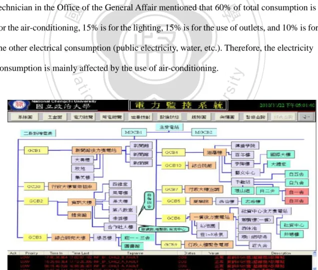
(28) Chapter 3. Real data analysis: Power. Consumption in National Chengchi University 3.1 Introduction Electricity is now an indispensable thing in our life. Without electricity, it is inconvenient to do everything. Recently with the concern of energy issue, we want to know how to reduce the use of power. Being a College of Commerce student in National Chengchi University, we concern about the electricity consumption for College of Commerce. 政治大 General Affair in Figure 3.1.立 The College of Commerce building is named “GCB5”. The. building. We collect the hourly data from the electricity monitor system in the Office of the. ‧ 國. 學. technician in the Office of the General Affair mentioned that 60% of total consumption is for the air-conditioning, 15% is for the lighting, 15% is for the use of outlets, and 10% is for. ‧. the other electrical consumption (public electricity, water, etc.). Therefore, the electricity. n. al. y. er. io. sit. Nat. consumption is mainly affected by the use of air-conditioning.. Ch. engchi. i n U. v. Figure 3.1 Plot of Electricity Monitor System 21.

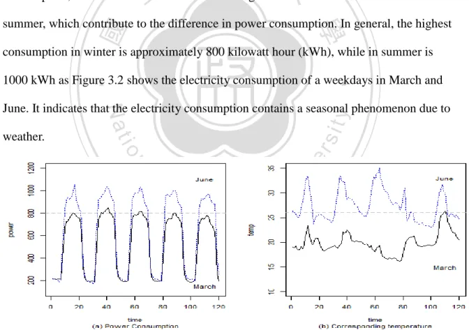
(29) We use the hourly data from 2008, February to 2009, January to construct the control and confidence bands and control charts. There are 52 weeks including the Spring Semester (from February to June ), Summer Vacation, Fall Semester(from September to January ), and Winter Vacation. The following we just discuss the days when students attend school. It is reasonable that we exclude the weekend (Saturday and Sunday), Summer Vacation and Winter Vacation data. Because we focus on the time when the electricity consumption will exceed the limits we determined, and try to find the cause that rises the consumption.. 3.2 Data classification. 政治大 of the air conditioning in winter is different from the use in consumption, while the use 立 Air-conditioning electricity consumption accounts for about 60% percent of the total. ‧ 國. 學. summer, which contribute to the difference in power consumption. In general, the highest consumption in winter is approximately 800 kilowatt hour (kWh), while in summer is. ‧. 1000 kWh as Figure 3.2 shows the electricity consumption of a weekdays in March and. y. sit. n. al. er. io. weather.. Nat. June. It indicates that the electricity consumption contains a seasonal phenomenon due to. Ch. engchi. i n U. v. Figure 3.2 Plot of the electricity consumption and corresponding temperature in March and June. 22.

(30) It shows that the highest consumption of the two months differ 200 kWk from part(a), while the temperature differs about 5℃ to 10℃ from part (b), so it can be inferred that temperatures may affect the electricity consumption. We use the temperature as the classification rule to divide our data into “Semester without Air-conditioner data” (denoted as WOAC data) and “Semester with Air-conditioner data” (denoted as WAC data). According to the Executive Yuan’ policy of energy conservation and carbon reduction, if the temperature doesn’t exceed 26℃, the office may not open the air conditioner. Due to temperature or climate changes (such as typhoons, cold), it may be. 治政大 So we use the also takes 26℃ as a standard to decide to open the Air conditioner. 立. suddenly cold or hot. Also the technician in the Office of the General Affairs of NCCU. rule ,“temperature exceed 26℃ from Monday to Friday”, as our premier grouping criteria.. ‧ 國. 學. Based on the Central Weather Bureau in Taipei station statistical data, if the data in the. ‧. semester (including Fall and Spring Semester), which depends on when the highest daily. sit. y. Nat. temperatures are all below 26℃ everyday in a weekday, is listed as WOAC; the remains. io. er. are divided to WAC data. Table 3.1 shows the period of WOAC data and WAC data. Regroup the data by using the procedures repeatedly until all the points fall in the control. al. n. v i n bands, confidence bands and control that all the weekdays’ data are C hlimits, which means engchi U in-control. We will illustrate them in section 3.3.. 23.

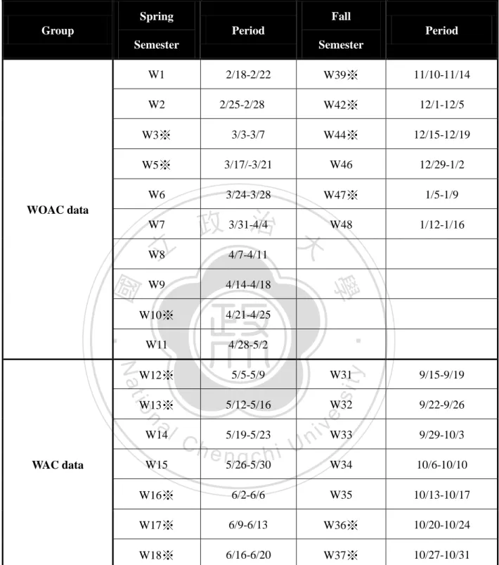
(31) Table 3.1 The grouping table Spring. Fall. Group. Period. Period. Semester. Semester W39※. 11/10-11/14. 2/25-2/28. W42※. 12/1-12/5. W3※. 3/3-3/7. W44※. 12/15-12/19. W5※. 3/17/-3/21. W46. 12/29-1/2. W6. 3/24-3/28. W47※. 1/5-1/9. W48. 1/12-1/16. W1. 2/18-2/22. W2. W7. 立. 4/7-4/11. 4/14-4/18. W10※. 4/21-4/25. W11. 4/28-5/2. Nat. W31. 9/15-9/19. W13※. 5/12-5/16. W32. 9/22-9/26. vW33. 9/29-10/3. W34. 10/6-10/10. Ch. 5/19-5/23. er. n. al. sit. 5/5-5/9. io. W12※. W14 WAC data. ‧. W9. 學. ‧ 國. W8. 治政 3/31-4/4 大. y. WOAC data. i n U. W15. e n5/26-5/30 gchi. W16※. 6/2-6/6. W35. 10/13-10/17. W17※. 6/9-6/13. W36※. 10/20-10/24. W18※. 6/16-6/20. W37※. 10/27-10/31. Note: In Table 3.1, “ ※” means that the weekday is from “No-Event Weekdays’ data”. The remaining are from ”Special-Event Weekdays’ data”.. 24.

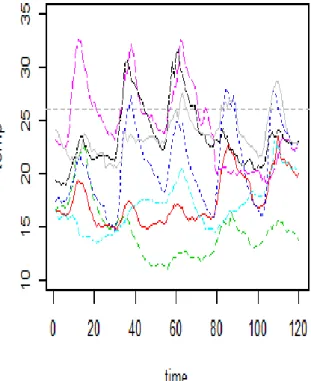
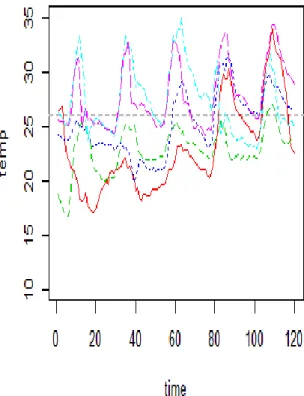
(32) According to calendar of National Chengchi University, after excluding the weekday that data exists the missing values, we divide the weekday data into “Special-Event Weekdays’ data” (denoted as SE data) and “No-Event Weekdays’ data”. (denoted as NE data) For SE data, it means that events occur such as national holidays, exam week, typhoons, etc. The occurrence of the events may affect the use of the electricity. For example, when the national holiday is coming, the number of students in the college of commerce building decrease and reduce the consumption of the electricity. Furthermore, when the day is hotter than usual, it is reasonable to see that the electricity consumption for the air-conditioning. 治政 so the consumption of electricity may not be affected by大 unusual incident. The 立. will be higher. For NE data, it means that no-special events could be found in that weekday,. establishment of the bands is based on the NE data, and use the bands to detect the SE data.. ‧ 國. 學. The following lists the plots for the WOAC data and WAC data. Figures 3.3 and 3.4. ‧. represent all the weekdays’ electricity consumption and the corresponding temperatures for. n. al. er. io. sit. y. Nat. NE data and SE data in WOAC dataset and WAC dataset, respectively.. Ch. engchi. 25. i n U. v.

(33) 立. 政治大. ‧. ‧ 國. 學. n. er. io. sit. y. Nat. al. Ch. engchi. i n U. v. Figure 3.3 Plot of power and corresponding temperature for NE data in WOAC data. 26.

(34) 立. 政治大. ‧. ‧ 國. 學. n. er. io. sit. y. Nat. al. Ch. engchi. i n U. v. Figure 3.4 Plot of power and corresponding temperature for SE data in WOAC data. 27.

(35) 立. 政治大. ‧. ‧ 國. 學. n. er. io. sit. y. Nat. al. Ch. engchi. i n U. v. Figure 3.5 Plot of power and corresponding temperature for NE data in WAC data. 28.

(36) 立. 政治大. ‧. ‧ 國. 學. n. er. io. sit. y. Nat. al. Ch. engchi. i n U. v. Figure 3.6 Plot of power and corresponding temperature for SE data in WAC data 29.

(37) 3.3 Phase I and Phase II control scheme When control and confidence bands and control charts are applied to data, there are two phases, Phase I and Phase II. Phase I is the period of building bands, including obtaining a set of in-control data and using them to construct the bands such that they can be used in Phase II. In this stage, “no-event weekdays” data are treated as in-control data and used to construct the confidence bands and control charts. Phase II is the period of using bands and control limits completed in Phase I to monitor the interested processes to understand whether they are in control. The confidence bands and limits we construct in Phase I are. 政治大 four monitoring methods in 立 Section 2, we use WOAC data and WAC data to construct the. applied to monitor the SE data, which is regard as the out-of-control data. According to. ‧ 國. 學. control and confidence bands and control charts, respectively. The procedure of constructing the charts and monitoring SE data are illustrated as follows.. Model assumption and identification. ‧. 3.3.1. sit. y. Nat. There are N weekdays in one group, which can be expressed “ith weekday ” , i=1, 2 ,…,N.. io. er. We collect hourly electricity consumption data and all the subgroups contain 120 observations, which can be denoted as 𝑥𝑡𝑖 , t=1,2,…,120. Obviously, there is seasonal. al. n. v i n influence and exists a daily cycleC ash shown in Figure 3.7, e n g c h i U so we fit the seasonal ARMA. model with period s=24. We can regard one peak as one day because of the daily cycle.. Figure 3.7 Plot of the electricity consumption 30.

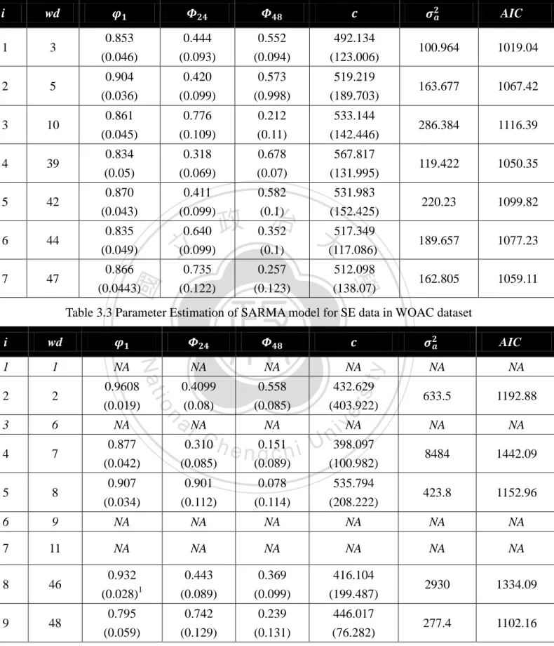
(38) In order to fit the suitable time series model, several models are selected as candidates. One of the most commonly used to determine the most “adequate” model is based on Akaike Information Criteria (AIC) ,which is defined as 𝐴𝐼𝐶 = −2 𝑙𝑜𝑔(𝑚𝑎𝑥. 𝑙𝑖𝑘𝑒𝑙𝑖ℎ𝑜𝑜𝑑) + 2𝑛𝑖 , where 𝑛𝑖 is the number of estimated model parameters. In the case of the ARMA(p,q) model we get 𝐴𝐼𝐶 = 𝑇 𝑙𝑜𝑔(𝜎̂𝑎2 ) + 2(𝑝 + 𝑞), By AIC, it is found that SARMA(1,0)×(2,0)24 is the best model for WOAC data : (1 − 𝜑1 𝐵)(1 − 𝛷24 𝐵 24 − 𝛷48 𝐵 48 )𝑥𝑡 = 𝑐 + 𝑎𝑡 , 𝑎𝑡 𝑖. 𝑖. 𝑑 𝑊𝑁(0, 𝜎𝑎2 ) ~. (3.1) 政治大 We use model (3.1) to fit WOAC 立 data. Table 3.2 lists the parameter estimation for NE data,. ‧ 國. 學. while Table 3.3 represents the parameter estimation for SE data. And SARMA(1,0)×(1,0)24 is a better model for each weekday for WAC data :. ‧. (1 − 𝜑1 𝐵)(1 − 𝛷24 𝐵 24 )𝑥𝑡 = 𝑐 + 𝑎𝑡 , 𝑎𝑡 𝑖. 𝑖. 𝑑 𝑊𝑁(0, 𝜎𝑎2 ) ~. Nat. y. (3.2). sit. We use model (3.2) to fit WAC data. Table 3.4 lists the parameter estimation for NE data,. n. al. er. io. while Table 3.5 represents the parameter estimation for SE data.. i n U. v. Model (3.1) and (3.2) are applied to analysis these weekdays for WOAC data and WAC. Ch. engchi. data, respectively. After model fitting, diagnostic check of residuals is performed to assess the suitability of the residuals. The results indicate that residuals follow a normal distribution. Figure 3.8 and Figure 3.9 show the plot of the autocorrelation function (ACF) and partial autocorrelation function (PACF) for the residuals by fitting model (3.1) and (3.2). Only the results of the four weekday’s observations are shown here, and the remains show similar patterns in the ACF and PACF plots.. 31.

(39) Table 3.2 Parameter Estimation of SARMA model for NE data in WOAC dataset 𝝈𝟐𝒂. i. wd. 𝝋𝟏. 𝜱𝟐𝟒. 𝜱𝟒𝟖. 𝒄. 1. 3. 0.853 (0.046). 0.444 (0.093). 0.552 (0.094). 492.134 (123.006). 100.964. 1019.04. 2. 5. 0.904 (0.036). 0.420 (0.099). 0.573 (0.998). 519.219 (189.703). 163.677. 1067.42. 3. 10. 0.861 (0.045). 0.776 (0.109). 0.212 (0.11). 533.144 (142.446). 286.384. 1116.39. 4. 39. 0.834 (0.05). 0.318 (0.069). 0.678 (0.07). 567.817 (131.995). 119.422. 1050.35. 5. 42. 0.870 (0.043). 0.411 (0.099). 0.582 (0.1). 531.983 (152.425). 220.23. 1099.82. 6. 44. 0.835 (0.049). 0.640 (0.099). 189.657. 1077.23. 7. 47. 0.866 (0.0443). 162.805. 1059.11. 立. 治 517.349 政 0.352 大(117.086) (0.1). ‧ 國. 0.257 (0.123). 512.098 (138.07). 學. 0.735 (0.122). AIC. Table 3.3 Parameter Estimation of SARMA model for SE data in WOAC dataset. NA. 2. 2. 0.9608 (0.019). 3. 6. NA. 4. 7. 0.877 (0.042). 5. 8. 6. io. 𝒄. NA. NA. NA. 0.4099 (0.08). 0.558 (0.085). 432.629 (403.922). n. a lNA Ch 0.310 (0.085). NA. e n g0.151 chi. y. 1. 𝜱𝟒𝟖. sit. 1. 𝜱𝟐𝟒. er. 𝝋𝟏. ‧. wd. Nat. i. i vNA n U 398.097. (0.089). (100.982). 𝝈𝟐𝒂. AIC. NA. NA. 633.5. 1192.88. NA. NA. 8484. 1442.09. 423.8. 1152.96. 0.907. 0.901. 0.078. 535.794. (0.034). (0.112). (0.114). (208.222). 9. NA. NA. NA. NA. NA. NA. 7. 11. NA. NA. NA. NA. NA. NA. 8. 46. 0.932 (0.028)1. 0.443 (0.089). 0.369 (0.099). 416.104 (199.487). 2930. 1334.09. 9. 48. 0.795 (0.059). 0.742 (0.129). 0.239 (0.131). 446.017 (76.282). 277.4. 1102.16. 1. “NA” means that data can’t fit time series model we determined, and it exists parameter estimation problem 32.

(40) Table 3.4 Parameter Estimation of SARMA model for NE data in WAC dataset j. Weekday. 𝝋𝟏. 𝜱𝟐𝟒. c. 𝝈𝟐𝒂. AIC. 1. 12. 0.803 (0.057). 0.977 (0.008). 565.574 (117.018). 615.7216. 1194.15. 2. 13. 0.836 (0.05). 0.991 (0.003). 535.237 (127.565). 200.553. 1081.27. 3. 16. 0.780 (0.062). 0.965 (0.012). 584.756 (107.503). 1002.518. 1242.68. 4. 17. 0.802 (0.057). 0.975 (0.008). 625.030 (125.592). 771.8483. 1219.77. 5. 18. 0.771 (0.062). 0.988 (0.004). 606.336 (110.34). 381.8266. 1152.17. 506.166. 1181.88. 393.5577. 1159.19. 37. 立. (0.051) 0.788 (0.059). 0.989 (0.004). 656.502 (130.405). 學. 7. 36. 政0.985 治 646.989 大 (0.005) (156.404). ‧. ‧ 國. 6. 0.830. y. 𝝈𝟐𝒂. AIC. sit. Table 3.5 Parameter Estimation of SARMA model for SE data in WAC dataset. NA. NA. 595.888 (84.347). 4425. 1391.95. NA. NA. NA. 2940. 1356.36. 𝜱𝟐𝟒𝒋. NA. NA. NA. 15. 0.702 (0.094). 0.878 (0.05). 3. 31. NA. 4. 32. 5. 2. al. 0.831. Ch. c. er. 14. n. 1. io. Weekday. Nat. 𝝋𝟏. j. eNA ngchi. i n U. v. 0.931. 691.624. (0.051). (0.02). (166.617). 33. NA. NA. NA. NA. NA. 6. 34. 0.943 (0.024). 0.921 (0.02). 493.153 (356.025). 1817. 1297.14. 7. 35. NA. NA. NA. NA. NA. 33.

(41) 立. 政治大. ‧ 國. 學. Figure 3.8 The ACF and PACF plots of residuals in WOAC data. ‧. n. er. io. sit. y. Nat. al. Ch. engchi. i n U. v. Figure 3.9 The ACF and PACF plots of residuals in WAC data 34.

(42) 3.3.2. Phase I and Phase II control charts. We introduce four methods which are (1) control bands under each time unit, (2) confidence bands based on Kalman Filter approach, (3) confidence bands based on Bootstrap approach, and (4) Hotelling T2 control charts. By using electricity consumption data in NCCU, we construct the Phase I control charts by NE data and monitor SE data for WOAC data and WAC data, respectively, and let α =0.0027 in the Phase I scheme. In Phase II, we apply the bands to monitor SE data, which is regard as out-of-control. SE data means that one or more events occur in the weekday such as national holidays, typhoons, abnormally high temperature, etc.. Table 3.6 represents the special event occurs in the weekday. We use this. 政治大. kind of data to evaluate the capability of four monitoring methods. When special events occur,. 立. we detect whether the electricity would be abnormal or not.. ‧ 國. 學 Special Event. 1. 2/18-2/22. Beginning weekday of Spring Semester. 2. 2/25-2/28. 228 Memorial Day. 6. 3/24-3/28. 7. 3/31-4/4. 9 11. WAC data. al. n. 8. y. sit. io. WOAC data. ‧. Period. Nat. weekday. none. Tomb Sweeping Day. er. Group. Table 3.6 Table of special events. Abnormal Temperature. 4/7-4/11. C h4/14-4/18 engchi U 4/28-5/2. v n i Abnormal Temperature Abnormal Temperature. 46. 12/29-1/2. New Year’s Day. 48. 1/12-1/16. Exam Week. 14. 5/19-5/23. NCCU Anniversary. 15. 5/26-5/30. Abnormal Temperature. 31. 9/15-9/19. Beginning weekday of Fall Semester. 32. 9/22-9/26. Abnormal Temperature. 33. 9/29-10/3. Typhoon. 34. 10/6-10/10. Double Tenth Day. 35. 10/13-10/17. none. 35.

(43) 3.3.3 I.. Example of Semester without AC data (WOAC data) Control bands under each hour. In Phase I, we calculate the control bands by equations (2.8) and (2.9). Figure 3.10part (a) shows the control bands under each time unit and the electricity consumption in weekday8 from SE data. All the observations from NE data fall in the bands, which means that the subgroups are from in-control. We can use this chart to monitor the data. In phase II, we plot the SE data into control bands (2.8) and (2.9). Table 3.7 shows the time points that electricity consumption are out of the control bands. It represents that eight of nine weekdays are detected to be out-of-control due to the special events. Only weekday 6 can’t. 政治大. be detected. We will discuss it in Section 3.4.. 立. To monitor the variance, we calculate the control bands of MS-bar by equation (2.9).. ‧ 國. 學. Figure 3.10 part (b) shows the control bands of MS under each time unit and the MS of weekday8 from SE data. All the MS from NE data fall in the bands, so we can use this chart. ‧. to monitor. In phase II, we plot the SE data into control bands. It represents that all the. y. Nat. n. al. er. io. sit. weekdays are detected to be out-of-control due to the special events.. Ch. engchi. 36. i n U. v.

(44) 政治大. 立. ‧. ‧ 國. 學 sit. y. Nat. n. al. er. io. Figure 3.10 Plot of control bands under each hour in Phase I for WOAC data. i n U. v. Table 3.7 Table of the OCC time point by control bands under each hour for WOAC data Weekday. Ch. e nOut-of-control g c h i time point (t). Weekday 1. 21, 40, 43, 44, 45, 46, 68, 69. Weekday 2. 1, 2, 47, 81~96. Weekday 6. None. Weekday 7. 43, 81~95, 105~ 119. Weekday 8. 38, 43, 57, 60, 62~69. Weekday 9. 62, 68, 69. Weekday 11. 62,81, 87~93, 105~109, 116, 117. Weekday 46. 67~70, 80~96, 103, 105~119. Weekday 48. 17,18, 20, 21, 22, 37~46, 54, 58~70, 81, 85, 87~89, 91~93,102 , 103, 105~118 37.

(45) II. Confidence bands based on Kalman Filter approach To construct the chart in Phase I scheme, we use the model (3.1) to apply to NE data. To the Kalman Filter method, the State-Space equation for each weekday can be expressed by (2.11) and (2.12) where φ1,i φ2,i Φi = ⋮ φ48,i [φ49,i. 1 0 ⋮ 0 0. 0 1. ⋯ ⋱. 0. A = (1. ⋯. 0 0 ⋮ 1 0]. 0 0 ⋯. 1 0 G= ⋮ 0 [0 ] 0). 政治大 The way to select initial values 立of 𝛼 ~𝑁(𝜇 , 𝑃 ) can refer to section 2.2.4. Using the R 2 𝑄𝑖 = 𝑅𝑖 = 𝜎̂𝑎𝑖 , i=1,2,…,7 0𝑖. 0𝑖. 0𝑖. ‧ 國. 學. functions “Kfilter0” and “Ksmooth0”, we get the estimate of the state variable 𝛼̂𝑡𝑖|𝑇 and 𝑃̂𝑡𝑖|𝑇 , i=1,2,…,7, t=1,2,…,120. Confidence bands can be calculated by (2.13) and (2.14). All. ‧. the fitted values fall in the confidence bands based on Kalman Filter approach. Figure 3.11. sit. y. Nat. shows the confidence bands based on Kalman Filter approach and the electricity. n. al. er. io. consumption in weekday8 from SE data.. v. In phase II, we apply model (3.1) to the SE data, and plot the fitted values of a profile into. Ch. engchi. i n U. equation (2.13) and (2.14). According to Table 3.3, the data of weekday1, weekday6, weekday9 weekday11 can’t be applied to model (3.1), so we plot the observations into the confidence bands. Table 3.8 shows the time points that fitted value of a profile are out of the bands. It represents that eight of nine weekdays are detected to be out-of-control due to some special events.. 38.

(46) Figure 3.11 Plot of CB based on Kalman Filter approach in Phase I for WOAC data. 政治大 Table 3.8 Table of the OOC立 time point by CB based on Kalman Filter approach for WOAC. Weekday 7. 80~95. ‧. Weekday 6. 12~22,37~ 41, 43~46, 63, 64, 67, 68, 69 None 32,33,43,45, 80~95, 104~ 119. Nat. y. Weekday 2. ‧ 國. Weekday 1. Out-of-control time point (t). 學. Weekday. Weekday 9. 57, 61, 62, 64, 65, 66, 68, 69. Weekday 11. 57, 61, 62, 63, 81, 84, 86~93, 105~109, 112, 113, 114, 117. Weekday 46. 67~70, 80~95, 104~119. Weekday 48. 12~22, 34~46, 57~70, 81~94, 105~118. er. n. al. sit. 37,38, 40~44, 57~69. io. Weekday 8. Ch. engchi. i n U. v. III. Confidence bands based on Bootstrap approach To construct the confidence bands in Phase I scheme, we use the model (3.1) to apply to NE data. We calculate the confidence bands by equations (2.15) and (2.16). Figure 3.12 shows the confidence bands based on Bootstrap approach and the electricity consumption in weekday8 from SE data. All the fitted values of profile for NE data fall in the bands. It means that the subgroups are in-control. We can use this confidence bands to monitor the future data of subgroups. In phase II, as we do in Kalman Filter approach, we plot the fitted 39.

(47) value of profile for SE data into equations (2.15) and (2.16). Table 3.9 shows the time points that the electricity consumption are out of the bands. It represents that eight of nine weekdays are detected to be out-of-control due to some special events.. 治政大in Phase I in WOAC data Figure 3.12 Plot of CB based on Bootstrap approach 立. Table 3.9 Table of the OOC time point by CB based on Bootstrap approach for WOAC. 12~22,38~ 41, 43~46, 63, 64, 65, 68, 69 23, 32, 43, 45, 80~95 ,106, 109 None. Nat. y. Weekday 6. Out-of-control time point (t). ‧. Weekday 2. ‧ 國. Weekday 1. 學. Weekday. Weekday 8. 37, 39~43, 58, 59, 60, 62~69. Weekday 9. 62~67, 69. Weekday 11. 62, 63, 81, 82, 84, 86~93, 105~109, 112, 113, 114, 117. Weekday 46. 23, 67~70, 80~95, 105~118. Weekday 48. 12~23, 34~46, 58~70, 81~94, 105~118. er. n. al. sit. 32,33,43,45, 81~95, 104~ 118. io. Weekday 7. Ch. engchi. i n U. v. To monitor the variance of residuals, Figure 3.13 part(a) shows the plots of the values of 𝜎̂𝑎𝑖 for each subgroup. The UCL is 15.71. One of the points exceeds the UCL from NE data. It is a false alarm case in the Phase I control chart. In phase II, from Figure 3.13 part (b), five of the nine weekdays’ data exceeds the UCL in s control charts, which indicate that these data are out-of-control. Fitting these data to the in-control model (3.1) leads to violating the stationary condition and reach no estimation results. Due to the parameter estimate problem 40.

(48) for the remaining four weekdays’ data (we denote “NA” in the control chart), we can’t fit them with the same in-control profile model in (3.1).. 政治大. 立. ‧. ‧ 國. 學. n. er. io. sit. y. Nat. al. Ch. engchi. i n U. v. Figure 3.13 Plot of standard deviation of the residuals in WOAC data IV. Hotelling T2 control charts Due to some of the values are very large, we take the logarithm to Hotelling T2 statistics in this section. Figure 3.14 shows the plots of the values of log(𝑇12 ) and log(𝑇22 ) statistics to monitor the coefficients of the profile and variance of residuals for NE data. The UCL for log(𝑇12 ) is 2.414 and the UCL for log(𝑇22 ) is 5.1396. All the statistics are under the upper limit, except for that the log(𝑇22 ) of weeday10 (wd10) exceeds UCL. It is a false alarm case in the Phase I control chart. So we can conclude that model (3.1) can be used as an in-control 41.

(49) profile data, and six of the seven weekday’s data are in-control data. To compute the values of log(𝑇12 ) and log(𝑇22 ) statistics, we use the corresponding estimates δ̅ and 𝜎̅𝑎2 in the Phase I scheme. From Figure 3.15, six of the nine weekdays’ data exceeds the UCL in both log(𝑇12 ) and log(𝑇22 ) control charts, which indicates that these data are out-of-control. The reason is that fitting these data to the in-control model (3.1) leads to violating the stationary condition and reach no estimation results. Due to the parameter estimate problem for the remaining three weekdays’ data (we denote “NA” in log(𝑇12 ) and log(𝑇22 ) control chart), we can’t fit the same in-control profile model (3.1) to. 治政大) statistics. They should have the for model (3.1), so we can’t calculate log(𝑇 ) and log(𝑇 立 get the estimation of coefficients. It is reasonable to infer that these weekdays are not suitable 2 1. 2 2. better time series model which is different from the in-control model (see Table 3.10), so they. ‧ 國. 學. can be identified to be out-of-control.. ‧. sit. y. Nat. Table 3.10 Table of the best time series model in Weekday1,6,9,11 for WOAC data wd. 9 11. n. 6. al. er. io. 1. Best seasonal time series model Sarima(1,0)×(1,0)24. i n C h Sarima(3,2)×(1,0) engchi U. v. Sarima(2,0)×(1,0)24 24. Sarima(1,0)×(1,0)24. 42.

(50) 立. 政治大. ‧ 國. 學. Figure 3.14 Plot of the values of log(T2) statistic for each weekday in Phase I for WOAC. ‧. data. n. er. io. sit. y. Nat. al. Ch. engchi. i n U. v. Figure 3.15 Plot of the values of log(T2) statistic for Special-Event Weekdays Data for WOAC data 43.

(51) 3.3.4 I.. Example of Semester with AC data (WAC data) Control bands under each hour. In Phase I, we calculate the control bands by equations (2.7) and (2.8). Figure 3.16 part (a) shows the control bands under each time unit and the electricity consumption in weekday32 from SE data. All the observations from NE data fall in the bands, which means that the subgroups are in-control. We can use this chart to monitor the data. In phase II, we plot the SE data together with control bands (2.7) and (2.8). Table 3.11 shows the time points that electricity consumption are out of the control bands. It represents that six of seven weekdays are detected to be out-of-control due to the special events. Only weekday 35 can’t be detected.. 立. 政治大. To monitor the variance, we calculate the control bands of MS by equations (2.9).. ‧ 國. 學. Figure 3.16 part (b) shows the control bands of MS under each time unit and the MS of weekday32 from SE data. All the MS from NE data fall in the bands, so we can use this. ‧. chart to monitor. In phase II, we plot the SE data into control bands. It represents that six of. y. Nat. sit. seven weekdays are detected to be out-of-control due to the special events. Only weekday. n. al. er. io. 35 can’t be detected as Table 3.11 shows.. Ch. engchi. 44. i n U. v.

(52) Table 3.11 Table of the OOC time point by control bands under each hour for WAC Weekday. Out-of-control time point (t). Weekday14. 24, 35. Weekday15. 67. Weekday31. 15, 22, 23, 24, 47, 50, 86, 87, 108~112. Weekday32. 11, 15~17, 33~43, 58~65, 83~89, 107~112. Weekday33. 9~23. Weekday34. 24, 105~118. Weekday35. None. 立. 政治大. ‧. ‧ 國. 學. n. er. io. sit. y. Nat. al. Ch. engchi. i n U. v. Figure 3.16 Plot of control bands under each hour in Phase I for WAC data. 45.

(53) II. Confidence bands based on the Kalman Filter approach To construct the chart in Phase I scheme, we use the model (3.2) to apply to NE data. To the Kalman Filter method, the State-Space equation for each weekday can be expressed by equations (2.11) and (2.12) where φ1,j φ2,j Φi = ⋮ φ24,j [φ25,j A = (1 0. 1 0 ⋮ 0 0. 0 ⋯. 0 1. ⋯ ⋱. 0. ⋯. 0 0 ⋮ 1 0]. 1 0 G= ⋮ 0 [0 ]. 2 , j=1,2,…,7 0), 𝑄𝑖 = 𝑅𝑖 = 𝜎̂𝑎𝑗. 政治大 functions “Kfilter0” and “Ksmooth0”, 立 we get the estimate of the state variable 𝛼̂. The way to select initial values of 𝛼0𝑖 ~𝑁(𝜇0𝑗 , 𝑃0𝑗 ) can refer to section 2.2.4. Using the R 𝑡𝑖|𝑇. and. ‧ 國. 學. 𝑃̂𝑡𝑖|𝑇 , i=1,2,…,7, t=1,2,…,120. Confidence bands can be calculated by equations (2.13) and (2.14). All the fitted values fall in the confidence bands based on Kalman Filter approach.. ‧. Figure 3.17 shows the confidence bands based on Kalman Filter approach in Phase I and the. sit. y. Nat. electricity consumption in weekday32 from SE data.. n. al. er. io. In phase II, we apply model (3.2) to the SE data, and plot the fitted values of a profile into. v. equations (2.13) and (2.14). According to Table 3.5, the data of weekday14, weekday31,. Ch. engchi. i n U. weekday33, weekday35 can’t be applied to model (3.2), so we plot the observations into the confidence bands. Table 3.12 shows the time points that fitted value of a profile are out of the bands. It represents that six of seven weekdays are detected to be out-of-control due to some special events. Only weekday35 can’t be detected.. 46.