JPEG2000 壓縮在雙核心數位訊號處理器上的實作

國

立

交

通

大

學

資訊學院資訊科技（IT）產業研發碩士專班

碩

士

論

文

JPEG2000 壓縮在雙核心數位訊號處理器上的實作與最佳化研

究

Implementation and Optimization of JPEG2000 Compression on Dual-core

DSP Processors

研 究 生：何柏瑲

指導教授：游逸平 教授

Implementation and Optimization of JPEG2000 Compression on Dual-core

DSP Processors

研 究 生：何柏瑲 Student：Po-Chiang Ho

指導教授：游逸平 博士 Advisor：Dr. Yi-Ping You

國 立 交 通 大 學

資訊學院資訊科技（IT）產業研發碩士專班

碩 士 論 文

A Thesis

Submitted to College of Computer Science National Chiao Tung University in partial Fulfillment of the Requirements

for the Degree of Master

in

Industrial Technology R & D Master Program on Computer Science and Engineering

July 2011

Hsinchu, Taiwan, Republic of China

i

JPEG2000 壓縮在雙核心數位訊號處理器上的實作

與最佳化研究

學生：何柏瑲

指導教授：游逸平 博士

國立交通大學資訊學院產業研發碩士專班

摘

要

多核心是未來處理器設計的趨勢。Analog Device (ADI)在最新一代的 Blackfin 處

理器—ADSP-BF561—中也採用了多核心的設計。BF561 是一顆採用微信號架構

(Micro Signal Architecture)的雙核心數位訊號處理器，此架構擅長於處理影像及各

種多媒體訊息。在本篇論文中，我們從 OpenJPEG 公開原始碼計畫中移植一個

JPEG2000 壓縮的程式到 BF561 上，接著在應用程式的階層上提出並實作最佳化

的方法。我們的最佳方法主要在於(一)資料地域性最佳化和(二)把工作分配到兩

個核心上執行。我們挑選了 JPEG2000 壓縮中佔運算比重最大的兩個部份—DWT

和 EBCOT Tier-1—來實行我們所提出最佳化方法。此外，我們在論文中討論實

驗中遇到的兩個關於編譯器的問題：其一是 GCC 內建函式對跨函式最佳化的干

擾，另一是 GCC 無法有效率的產生出平行指令。在我們的實驗中，我們發現使

用我們所提出的資料地域性最佳化後可以有效地提昇兩個核心的使用效率，原因

是我們的最佳化幅度減少了對外界低速記憶體存取的需求。我們使用了四張標準

的測試影像來評估我們最佳化的效能。我們的最佳化結果相較於原始程式在一個

核心上執行並加了-O3 編譯器最佳化，可以加速影像壓縮達 1.92 至 2.04 倍左右。

ii

student：Po-Chiang Ho

Advisors：Dr. Yi-Ping You

Industrial Technology R & D Master Program of

Computer Science College

National Chiao Tung University

ABSTRACT

Multi-core is the trend of future processor design. Along with this trend, Analog Device

(ADI) developed their latest Blackfin processor–ADSP-BF561–with a multi-core design.

BF561 is a dual-core, SMP-like DSP processor based on micro signal architecture (MSA),

which is specialized for video processing and multimedia computations. In this paper we

propose several software-level optimizations to speed up a JPEG2000 compression program

ported from OpenJPEG project on a Blackfin BF561 processor. Two optimization methods,

data locality optimization and utilization of two cores, are performed on the two

heavy-loading stages of JPEG2000 compression: DWT and EBCOT Tier-1. Implementation

issues such as the disturbance to compiler optimizations when using GCC attributes and

inefficient generations of parallel instructions are discussed. In our experiments, we found

that we can only benefit from the utilization of two cores after the data locality optimization is

well performed because the data locality optimization reduces the heavy loading of accesses to

low-speed SDRAM. Four popular image testbenches are used to evaluate the efficiency of our

optimizations. The experiments showed that the optimizations have a speed-up of

1.92x–2.04x for the compression compared to the baseline with -O3 optimization flag running

on single core.

iii

誌 謝

1 Introduction 1 1.1 Overview . . . 1 1.2 Motivation . . . 2 1.3 Problem Definition . . . 3 1.4 Contribution . . . 4 1.5 Thesis Organization . . . 5 2 Related Work 6 3 JPEG2000 Overview 9 3.1 Background and History . . . 9

3.2 JPEG2000 Compression Procedure . . . 11

3.2.1 Pre-processing . . . 12

3.2.2 Discrete Wavelet Transform . . . 13

3.2.3 EBCOT Tier-1 Coding . . . 16

3.2.4 EBCOT Tier-2 Coding . . . 20

4 The Architecture of Analog Device BF561 21 4.1 Blackfin Core . . . 21

4.2 Blackfin ADSP-BF561 . . . 23

4.2.1 Memory Hierarchy . . . 24 iv

4.2.2 DMA Support . . . 25

5 Implementation and Optimization 28 5.1 Experiment Environment Setup . . . 28

5.2 Software-based JPEG2000 Implementation and Profiling . . . 29

5.3 Overview of JPEG2000 Optimizations on BF561 . . . 30

5.3.1 Data Locality Optimization . . . 30

5.3.2 Utilization of Two Cores . . . 33

5.4 Optimization of DWT . . . 36

5.4.1 Data Locality Optimization . . . 36

5.4.2 Utilization of Two Cores . . . 40

5.4.2.1 Data Partition . . . 40

5.4.2.2 Task Partition . . . 42

5.4.3 DMA Optimization . . . 45

5.5 Optimization of EBCOT Tier-1 . . . 47

5.5.1 Data Locality Optimization . . . 47

5.5.2 Utilization of Two Cores . . . 50

5.6 Optimization Using Inline Assembly . . . 51

6 Evaluations and Discussions 53 6.1 Evaluations and Discussions of DWT . . . 53

6.2 Evaluation and Discussion of EBCOT Tier-1 . . . 56

6.2.1 The Disturbance of Compiler Optimizations due to Putting Proce-dures to the L1 Instruction SRAM . . . 60

6.3 Evaluation of Inline Assembly Optimization . . . 61

6.4 Overall Evaluation . . . 62

6.4.1 Data Cache V.S. Handmade Data Locality Optimization . . . 64 v

7.1 Summary . . . 68 7.2 Future Work . . . 69

List of Figures

3.1 The procedure of JPEG2000 lossless compression. . . 12

3.2 (5,3) DWT (left) and inverse DWT (right). . . 14

3.3 An example of discrete wavelet transform: (a) the original image, (b) after 1D-DWT computation in horizontal direction, (c) after 2D-DWT compu-tation, (d) 2-level DWT computation. . . 14

3.4 The ordering of high pass coefficients and low pass coefficients being gen-erated. . . 16

3.5 The hierarchy of data partition of an image. . . 17

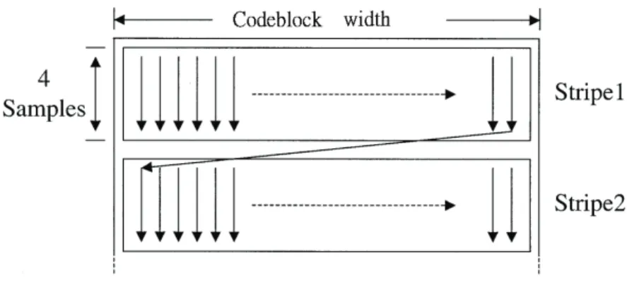
3.6 The scan pattern of a codeblock in one bit-plane. . . 18

3.7 An example to show what is “significant”. . . 18

3.8 The hierarchy of bit-plane coding. . . 18

4.1 Blackfin core architecture. . . 22

4.2 Block diagram of BF561 architecture. . . 23

4.3 Memory and bus architecture of BF561. . . 27

5.1 Execution time breakdown of JPEG2000 compression on the BF561 pro-cessor. . . 31

5.2 Master-slave model of MPEG-2 encoder on dual-core processors. . . 34

5.3 Pipelined model of MPEG-2 encoder on dual-core processors. . . 35

5.4 2D-DWT computation. . . 37 vii

5.7 The data moving flow in a vertical line. . . 40

5.8 Dataflow of DWT computation performed in one line: (a) before data lo-cality optimization (b) after data lolo-cality optimization. . . 41

5.9 The data partition to two cores. . . 42

5.10 The memory/calculation partition to two cores . . . 43

5.11 Latency of DMA transfer in continuous data. . . 46

5.12 Linking of DMA despriptors. . . 46

6.1 The analysis of time consumption in DWT before and after data locality optimization. . . 55

6.2 The analysis of execution time of DWT using mem/cal partition. . . 57

6.3 Speed-up of the proposed optimizations for DWT. . . 57

6.4 Speed-up of the proposed optimizations for EBCOT Tier-1. . . 59

6.5 A simple program to show the disturbance of compiler optimizations due to putting procedures to the L1 instruction SRAM. . . 61

6.6 The assembly codes of the simple test program in Figure 6.5. The left is the original one; the other is the disturbed one. . . 62

6.7 The MCT source code. . . 63

6.8 The assembly code generated by GCC. . . 63

6.9 The assembly code we reassembled. . . 64

6.10 The performance comparison between automatic data cache and our hand-made data locality optimization. . . 65

6.11 Time consumption to compress a 640x480 image. . . 66

6.12 The standard image testbenches. . . 66

6.13 The overall performance evaluation of proposed optimizations on standard image testbenches. . . 67

3.1 An example of the three coding passes being performed in every bit-plane. 19 5.1 The data allocation of EBCOT Tier-1 in the L1 data SRAM. . . 49 6.1 DWT: The evaluation of performance improvements of two optimizations:

data locality optimization and utilization of two cores. . . 53 6.2 The loading comparison between memory transfer and computations in

DWT. . . 56 6.3 EBCOT Tier-1: The evaluation of performance improvements of two

opti-mizations: data locality optimization and utilization of two cores. . . 58

Chapter 1

Introduction

1.1

Overview

Digital images or videos need large amounts of space for storage of the contents. For the efficient utilization of memory and storage space, we need to compress them via reducing spacial or temporal redundancy. Image (video) compression is a digital signal process-ing technique developed to compress an image (video). The compression procedures have heavy computation and calculation loading. In a desktop environment, this is not hard be-cause the computing power of modern CPUs often could afford the loading. However, in an embedded environment, power consumption often needs to be considered since power supply of many embedded systems come from batteries. Application-specific integrated circuit (ASIC) is a good choice for speed and power consumption, and the price are often not expensive. DSP processors may be another flexible choice since they could run soft-ware programs just like we run on desktop. Although the performance are not good as ASIC, DSP processors are convenient to change software programs to target specific appli-cations and the performance on image compression are often better than general purpose processors.

DSP processors are microprocessors designed to perform digital signal processing, the mathematical manipulation of digitally represented signals. Digital signal processing is one of the core technologies in rapidly growing application areas such as wireless

tions, audio and video processing, and industrial control [9]. Powerful ALUs and Multipli-ers are the basic characteristics of DSP processors and their memory access often could be parallel with mathematic calculations. Furthermore, special hardware components are de-signed on them for accelerating digital signal processing like subtract-absolute-accumulate (SAA), multiplier-and-accumulation (MAC), and so on.

JPEG2000 [15] is a novel image standard proposed by JPEG committee to approach the modern applications such as Internet, medical images, video conference and etc. Hence, we do some researches to examine that how JPEG2000 could benefit from the architectures of modern DSP processors.

1.2

Motivation

Moore’s law tell us that the number of transistors that can be put on an integrated circuit has doubled approximately every two years. The trend has continued for more than half a century. It will stop, however, eventually on a certain level and cannot go on any more since the atomic limit. In addition, there are two serious problems while we try to put more transistors on a chip: overheat and power consumption. Therefore, processors are designed multi-cores, which means to put one more cores on one chip. Hence, how to divide calculating jobs to many cores becomes an important issue.

To follow this trend, the newest DSP processors of Blackfin family, which are devel-oped by Analog Device (ADI), are also designed multi-core; that is ADSP-BF561 [3].

Blackfin 16/32-bit embedded processors are designed for software flexibility and scala-bility for convergent applications: multi-format audio, video, voice and image processing, multi-mode baseband and packet processing, control processing, and real-time security. ADSP-BF561 is configured as a symmetric multiprocessing arrangement of two Blackfin processor cores. Each is capable of operating at up to 600 MHz and has up to 2.6 MB of on-chip SRAM memory.

CHAPTER 1. INTRODUCTION 3 Why we choose Blackfin? There are some reasons make it distinctive. Blackfin archi-tecture is named micro signal archiarchi-tecture (MSA); it’s co-developed by Intel and Analog Device. Unlike very long instruction word (VLIW) architecture, MSA mixes powerful ALUs into RISC-like processors. This leads several advantages. First, RISC architecture is known compiler friendly. Hence, compiler designs for MSA are easier than for VLIW, which is adapted by most DSP processors. In addition, the design flow is straightforward; the two suites of development tools aren’t needed. Finally, the hardware designs are more cost and power effective.

In recent years, surveillance cameras and automatic traffic recorders (ATR) are popular and widely used in our daily life. To reach better compression video quality, we need a novel video compression standard.

JPEG2000, a new compression standard for still images, is developed to overcome the shortcomings of the existing JPEG standard, which is standardized by Joint Technical Committee on Information technology of the International Organization for Standardiza-tion (ISO)/InternaStandardiza-tional Electrotechnical Commission (IEC).

In JPEG2000 standard, Motion JPEG2000 has been standardized to be a part of JPEG2000. It could be used as video standard to achieve better video quality for widely uses include cinema, surveillance, ATR and so on.

For the reasons mentioned above, we try to examine how JPEG2000 software based compression could efficiently run on a dual-core BF561 to achieve good compression per-formance.

1.3

Problem Definition

Since we know ADSP-BF561 is a dual-core processor, and uClinux could run on both cores like symmetric multi-processor (SMP). uClinux is a lightweight version of Linux working on processors with no memory management unit (MMU) and the trunks for BF561

are developed by the community. If we have full uClinux supports on BF561, we have affluent library supports from Linux. This makes easy for us to establish our own image compressing systems. In addition, abundant resources about Linux also could be found on the Internet.

However, there are still lacks of researches and reference manuals to discuss the utiliza-tion of two cores. We need to know if jobs’ partiutiliza-tion to two cores in BF561 could as good as in general SMP. If it works well, we are convenient to move our software development procedures in a general SMP system to this SMP-like system.

For these reasons, we implement and optimize JPEG2000 on BF561. We divide JPEG2000 into several components and do the parallelization on these components.

Our JPEG2000 compression program would be expected to totally come from open-source reopen-sources. To exploit famous open-open-source projects from the Internet, we are not only easy to build our experimental environments but also capable to learn the source code implementations. Furthermore, they may be allowed to be commercial utilization; this depends on their release Licenses. Our JPEG2000 compression would be focused on lossless compression since it could conserve the details for flexible utilization.

Our optimization approaches would derivate from the convergence of profiling, the understanding of JPEG2000 algorithms, and hardware architectures; the optimization or-dering would follow the principle: the efficient one, the prior one.

1.4

Contribution

In this paper, we implement and optimize the JPEG2000 lossless compression under SMP-like mode on Analog device BF561. Our optimizations focus on the components of JPEG2000, DWT and EBCOT Tier-1, which are the heavy loading and also potential parallel parts of the whole compression procedure. Our main contributions list in the following:

CHAPTER 1. INTRODUCTION 5 supports on BF561 SMP-like environments.

• Implementation and evaluation of data locality optimization by using high-speed L1

data SRAM

• Implementation and evaluation of jobs’ partition to dual cores.

• Implementation and evaluation of the effectiveness of inline assembly optimization

on JPEG2000.

1.5

Thesis Organization

This thesis is organized as follow. In chapter 2, the related work is introduced. In chap-ter 3, we describe the overview of JPEG2000. In chapchap-ter 4, we describe the architecture of Blackfin BF561, the target platform of this work, especially on the memory architec-ture and DMA supports. In chapter 5, we detailed discuss the implementations and our optimization methods of JPEG2000 on BF561. In chapter 6, the experimental results is presented and the problems we encountered is discussed. The chapter 7 concludes the work and presents future work.

Related Work

There are several researches about JPEG2000. Majif Rabbain and Rajan Johsi gave a very good overview of JPEG2000 [22]; it’s a good beginning to understand JPEG2000. David Taubman and Michael Marcellin have deeply discussed the theory of digital signal pro-cessing techniques used in JPEG2000 [25]. Timku Acharya and Ping-sing Tsai detailedly explained the specifications of JPEG2000 [2]. They focused on the specifications and im-plementations. In addition, many good examples are included. It is a very good reference to understand the implementation details of JPEG2000.

There are also many studies about JPEG2000 software implementations on different processors. H. Muta et al. did implementation and parallelizations of JPEG2000 com-pression on Cell/B.E [19]. They speeded up the JPEG2000 encoding by parallelizations using SPEs on the Cell/B.E. In addition, they did the system level parallelizations by using Cell/B.E blade servers. P. Meerwald et al. evaluated parallelizations of JPEG2000 using OpenMP and JAVA threads on SMP Intel Pentium II Xeon running at 500 MHz [17]. The tile parallelization was abandoned here due to the artifact effects. The JAVA implemen-tation was from JJ2000 and the OpenMP was adpated in the C implemenimplemen-tation of Jasper. The parallelization results showed that they could avoid cache missing greatly if the image was read from the vertical directions. In addition, EBCOT Tier-1 was encoded by parallel codeblocks. Azkarate-Askasua Mikel built a JPEG2000 compression system in a

CHAPTER 2. RELATED WORK 7 processor system on FPGA using the commercial system-level-design tool [7]. They used OpenJPEG library to be the JPEG2000 implementation and divided it into several parts in order to map them on to the design tool. System-level-design tools are used to reduce the efforts of developers and speed up the time to market.

Discrete wavelet transform (DWT), which is an important component of JPEG2000 compression, suffers memory uncontinuous reading problems while using software im-plementations. Dividing the image into pseudo small tiles is the solution used in [19]. However, in order to avoid edge effects, they have to make the tiles overlapping. This work needs large efforts. Putting the vertical lines together and then performing DWT to them using JAVA threads is the solution used in [17]. However, we don’t have a JAVA environ-ment and Linux threads cannot be scheduled to the other core on BF561. In our solution, we analyze the model of uncontinuous memory accesses and transform theses accesses to be the jobs of DMA controllers. Then, DMA controllers help transform these data to be continuous data and put them in the high speed SRAM for fast accesses. Our work can efficiently eliminate the slow accesses to external SDRAM.

In addition, there are several with respect to Blackfin platforms. Michael G. et al. put data in shared L2 SRAM of BF561 and performed the data processing from both cores [8]. They showed that to put the data in the SRAM could only benefit from the stream pro-gramming model. The model means that the two cores do different jobs. Jun-Wei Gao and Ke-Bin Jia established a H.264 based video surveillance system with real-time compression on a BF561 platform [13]. They briefly described five methods to optimize the h.264 en-coder: (1) allocating storage space , (2) issuing parallel instructions ,(3) using special video instructions ,(4) utilizing hardware loop ,and (5) choosing a suitable assembly instruction. Hee Seo and Seon Wook Kim improved OpenMP performance on BF561 by moving shared data into shared L2 SRAM and further moving private data into L1 SRAM [23]. They fo-cused on the fork/join model and put the data into L1 data SRAM as possible as they can;

only shared variables stayed in shared L2 SRAM. They showed that the power consump-tion could be reduced by directly measurement using external sourcemeters. C.H. Chen showed that well-optimized Blackfin assembly code could achieve high performance im-provement compared to unoptimized one [11]. The assembly of Blackfin architecture can be parallelized under some restrictions. They used the feature to reassemble the assembly to speed up the discrete wavelet transform in JPEG2000.

The related work mentioned above include many aspects of researches. Some of these work mentioned that how they optimized their implementations on the Blackfin platform. These work can be references for us to avoid going the wrong ways in our researches.

Chapter 3

JPEG2000 Overview

In this chapter, we will introduce the basic concepts of JPEG2000 and explain why it is special and different from traditional JPEG.

3.1

Background and History

The well-known JPEG standard is developed by JPEG (Joint Photographic Experts Group) committee, which is founded in 1986 under the joint auspices of ISO and ITU-T, and has become the most popular image compression standard in past twenty more years. Almost every image or video instrument supports JPEG standard. Despite the great success of the JPEG image compression system, it has several shortages that become increasingly apparent as the need for image compression is extended to emerging applications such as medical imaging, digital libraries, Internet multimedia transmission, and so on.

In March 1997 a call for proposals was issued to the new standard—JPEG2000. In November 1997, more than 20 algorithms were evaluated [22]. Finally it included many classic algorithms and became a “big” standard. Nowadays, JPEG 2000 refers to twelve parts of the standard [15]:

• Part 1 Core coding system (intended as royalty and license-fee free — NOT

patent-free)

• Part 2 Extensions (adds more features and sophistication to the core) • Part 3 Motion JPEG2000

• Part 4 Conformance

• Part 5 Reference software (Java and C implementations are available)

• Part 6 Compound image file format (document imaging, for pre-press and fax-like

applications, etc.)

• Part 7 has been abandoned • Part 8 JPSEC (security aspects)

• Part 9 JPIP (interactive protocols and APIs) • Part 10 JP3D (volumetric imaging)

• Part 11 JPWL (wireless applications)

• Part 12 ISO Base Media File Format (common with MPEG-4)

Part 1 (the core) is now published as an International Standard , five more parts (2-6) are complete or nearly complete, and four new parts (8-11) are under development.

While the standard is well defined, why we need JPEG2000? There must be some reasons to persuade us to use the new standard. There are several new features show that why JPEG2000 could be the compression standard of the next generation [2]:

1. Superior low bit-rate performance—JPEG2000 offers good performance in very low bit-rates compared to traditional JPEG.

2. Large dynamic range of the pixels—JPEG2000 is the only standard could conduct the pixel values more than 16-bit precision; it is up to 38 bits;

CHAPTER 3. JPEG2000 OVERVIEW 11 3. Lossless and lossy compression—JPEG2000 provides lossless compression with progressive decoding. Applications such as digital libraries/databases and medical imagery can benefit from this feature.

4. Protective image security—the open architecture of the JPEG2000 standard makes easy the use of protection techniques of digital images such as watermarking, label-ing, stamping or encryption.

5. Region-of-interest coding—in this mode, regions of interest (ROIs) can be defined. These ROIs can be encoded and transmitted with better quality than the rest of the image.

6. Robustness to bit errors—the standard incorporates a set of error resilient tools to make the bit-stream more robust to transmission errors.

Because of the good design of JPEG2000, it could be used in a variety of applications from professional medical images, Internet, wireless transmission, to low-end consumer electronics.

3.2

JPEG2000 Compression Procedure

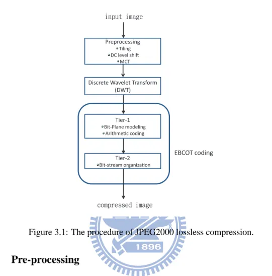
In this section, we discuss about the JPEG2000 Part1 standard, the core of JPEG2000. We focus on the procedure of lossless compression of JPEG2000 since the lossless com-pression could reserve more details for flexible utilization. The main components of the coding procedure could be divided into four parts: pre-processing, discrete wavelet

trans-form, EBCOT Tier-1 and EBCOT Tier-2, as shown in Figure 3.1. We will discuss these

Preprocessing

Tiling DC level shi!

MCT

Discrete Wavelet Transform (DWT) Tier-1 Bit-Plane modeling Arithme"c coding Tier-2 Bit-stream organiza"on EBCOT coding joqvu!jnbhf dpnqsfttfe!jnbhf

Figure 3.1: The procedure of JPEG2000 lossless compression.

3.2.1

Pre-processing

The pre-processing state includes three passes: tiling, Direct Current (DC) level shift and color transformation . In the first pass, tiling, we may partition the whole image into several independent “tiles”, and these tiles could be encoded by the independent parameters in the following procedures. This is useful when the compression hardware system has limited memory. The tiling size theoretically could be any size but often 512x512 or bigger up to the whole image size since small tiling size would lead to obvious edge effects [2].

After titling, we perform DC level shift to shift pixel values from unsigned value to signed value in order to make the pixel values more balanced in the distance to “zero”; this leads more “zero” while quantization is performed and the compression ratio could be higher. Finally, we make color transformation called Multi-component Transformation (MCT) to transfer the color space of the image from RGB color space to YUV color space.

CHAPTER 3. JPEG2000 OVERVIEW 13 There are two kinds of MCT in JPEG2000 specification, which are Reversible Color Trans-formation (RCT) and Irreversible Color TransTrans-formation (ICT). RCT is applied in reversible coding and ICT is used in irreversible coding.

3.2.2

Discrete Wavelet Transform

The purpose of Discrete Wavelet Transform (DWT) is the same with discrete cosine trans-form in traditional JPEG but in different coding system. It tries to divide high frequency parts and low frequency parts of an input image so that we could adapt different strategies in the following steps to increase compression ratio. The “low frequency” could be real-ized that the values of two adjacent pixels of an image are similar. If the pixel values of a small region are similar, this region would be “smooth” as we view. The low frequency parts occupy the majority of a common natural image. On the other hand, “high frequency” implies that there may exist a shape, edge, or line or conceal more details.

The technique of DWT in JPEG2000 is based on filters. There are one high pass filter and one low pass filter in it. Low pass filter reserves low frequency data, which occupy most parts of an general natural image. On the other hand, high pass filter reserves high frequency data.

Two kinds of DWT filter are included in JPEG2000 standard: (9,7) and (5,3). The number “9” means the length of low pass filter is 9 and the number “7” means the length of high pass filter is 7. Since we focus on reversible coding, we just examine the (5,3) filter, which is designed for reversible coding, in the following discussion.

The (5,3) DWT and its opposite version, inverse DWT, are illustrated in Figure 3.2 [22]. The left site of the Figure 3.2 is DWT (forward) and the right one is inverse DWT. Input sequences x(n) are conducted by low pass filter h0(n) and high pass filter h1(n) and then

followed by sub-sampling of factor 2 to get output data; we call these output data ”DWT

coefficients”. On the other hand, these DWT coefficients could be reconstructed to original

Figure 3.2: (5,3) DWT (left) and inverse DWT (right).

(a)

(d) (c)

(b)

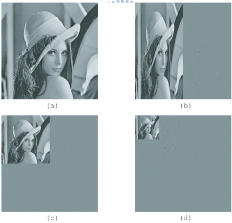
Figure 3.3: An example of discrete wavelet transform: (a) the original image, (b) after 1D-DWT computation in horizontal direction, (c) after 2D-DWT computation, (d) 2-level DWT computation.

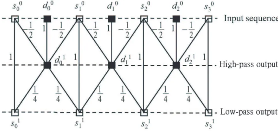
CHAPTER 3. JPEG2000 OVERVIEW 15 The DWT computation of JPEG2000 is 2D-DWT; it means we do the DWT on an image from column by column to row by row. The ordering could be inverse from row by row to column by column. The effects on an image before and after 2D-DWT could be seen in Figure 3.3. Figure 3.3(a) is the original classic test patent: 512x512 gray-scale Lena. Figure 3.3(b) shows that the input image is separated to low frequency in left side and high frequency in right side after 1-D horizontal DWT computation; then we do the DWT computation to separate high and low frequency data in vertical direction, as shown in Figure 3.3(c). Furthermore, We could perform a two-level DWT for the low frequency data, as shown in Figure 3.3(d); it’s level 2.

The traditional DWT needs complex convolution computations and is not adapted in JPEG2000 standard. JPEG2000 adapts a lifting-based DWT [12], which reduces signif-icant memory footprint and computing complexity compared with traditional DWT. Fur-thermore, it could run in place; this means no more other memory space is needed during the computation, and the input data and the output data use the same memory space. The lifting-based DWT is based on two steps: prediction and updating. The Equation 3.1 shows that how to make the prediction calculation. {s0

} and {d0

} means even and odd values of

input sequence, respectively. {d1

} refers to the output of high pass coefficients. The

up-dating procedure is shown in Equation 3.2; the output of low pass coefficients {s1 } are

obtained by specific calculation of modified coefficients {d1

} and input data {s0

}. The

subscript “i” means the input number. The concept could be expressed by Figure 3.4 [22]. We could see the ordering that high pass coefficients and low pass coefficients are inter-leaved generated. d1_{i = d}0_{i −}1 2(s 0 i + s 0 i+1) (3.1) s1_{i = s}0_{i +}1 4(d 1 i₋₁+ d 1 1) (3.2)

Figure 3.4: The ordering of high pass coefficients and low pass coefficients being gener-ated.

3.2.3

EBCOT Tier-1 Coding

After DWT computation, the JPEG2000 compression enters the entropy coding,

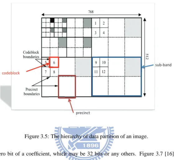
Embed-ded Block Coding with Optimal Truncation (EBCOT) coding. EBCOT coding is diviEmbed-ded

into two steps: Tier-1 and Tier-2. Tier-1 coding divides the DWT coefficients to several non-overlapping blocks and then encodes each of the blocks independently; we call these blocks “codeblocks”. Besides codeblocks there are several blocks defined hierarchically for efficient coding in Tier-2. The whole data partition scenario could be illustrated in Fig-ure 3.5. We see that the image is separated into sub-bands; then each sub-band is divided into several precincts; then each precinct is divided into several codeblocks. The code-block size could be any size but the power of 4. However, the size often is 32x32 or 64x64 because the performance is better [2].

Since the basic coding element is codebclock, a codeblock is encoded in the elements of “bit-plane”. The three coding passes are performed to encode the bit-level data in a bit-plane; the encoding ordering in a bit-plane is followed by scanning of 4 subsequent bits as shown in Figure 3.6 [16]. The bit-plane coding is stared from the most significant bit (MSB) to least significant bit (LSB) of the coefficients in this codeblock. Actually, it starts from which any bit in this bit-plane is significant. The “significant” means the first

CHAPTER 3. JPEG2000 OVERVIEW 17

sub-band

precinct

codeblock

Figure 3.5: The hierarchy of data partition of an image.

non-zero bit of a coefficient, which may be 32 bits or any others. Figure 3.7 [16] is an example to show what is “significant”. The figure 3.8 [16] shows that the hierarchy of the coding elements in a codeblock. We could see that the least basic element is “a bit”.

The three coding passes performed in a bit-plane are:

• Significant Propagation Pass (SPP): This is the first coding pass used in one

bit-plane except the first bit-bit-plane of the codeblock. This coding pass is adapted if this bit is a preferred bit, which means eight of its adjacent bits are already in significant state.

• Magnitude Refinement Pass (MRP): This coding pass is applied after the first “1”

bit of this coefficient has been encoded and the bit now is 1.

Figure 3.6: The scan pattern of a codeblock in one bit-plane.

Figure 3.7: An example to show what is “significant”.

CHAPTER 3. JPEG2000 OVERVIEW 19 coefficient value coding pass 21!!!!!2!!!!!4!!!!!.7 cleanup 1+ 0 0 0 significance refinement cleanup 0 0 0 1-significance refinement cleanup 0 1+ 1 1 significance refinement cleanup 1+ 0 1 1

Table 3.1: An example of the three coding passes being performed in every bit-plane. and MRP except the first bit-plane. The first pit-plane starts coding from CUP. Table 3.1 shows an example that how the 4 coefficients are encoded in every bit-plane. The every bit-plane is encoded via three coding passes and the a bit is encoded in one of the coding passes. Where a bit should be coded is following a sequence of conditional ad-justments. The adjustments include four coding operations. When to use these operations bases on some conditions are satisfied. The four coding operations are:

• Zero Coding (ZC): ZC encodes a bit according to that if the neighbors of the bit are

already in significant state. If one’s neighbors are already in significant state, it is very likely to be significant.

• Sign Coding (SC): SC records the sign information of a coefficient and its adjacent

4 coefficients (right, left, up, down).

• Magnitude Refinement Coding (MRC): MRC is applied after a coefficient is already

in significant state; in other words, there its first non-zero bit has already been coded.

• Run-Length Coding (RLC): RLC is used to encode the consecutive four bits in a

vertical scanning pattern; how many bits should be encoded depends on where the first non-zero bit exists.

Since we know every bit-plane is coded in three passes with four operations, this com-plicated mechanism will not be detailed discussed. The detailed procedures can be found in [2].

After the three coding passes are generated, these coding passes are encoded using binary arithmetic coding, MQ-coder. Arithmetic coding is a superior efficient coding ar-chitecture compared to traditional Huffman coding in JPEG and can tackle binary input data. It rescales probability interval when a input datum is coming in according to the appearing probability of the datum. The arithmetic coding applied in JPEG2000 is MQ-coder. MQ-coder is a kind of adaptive arithmetic coding; it means that the encoding site changes its probability prediction synchronizing with the decoding site. The probability prediction changes following the input data with look-ups to a fixed constant table. MQ-coder divides the probability interval into two sub-intervals: more probable symbol (MPS) and less probable symbol (LPS). The two sub-intervals indicate that the input symbol, 1 or 0, which is more probable to happen. If the input symbol is in the LPS interval, the output codeword will be updated according to the estimation table.

3.2.4

EBCOT Tier-2 Coding

The purpose of 2 coding is that how to efficiently organize the encoded data of Tier-1 . The main works of Tier-2 are to represent the layer and block summary information for each codeblock. A layer consists of consecutive bit-plane coding passes from each codeblock in a tile, including all the sub-bands of the components in the tile. The block summary information consists of lengths of compressed code words of the codeblock, the most significant magnitude bit-plane at which any sample in the codeblock is non-zero, and the truncation point between the bit-stream layers among others [2]. Then, these infor-mation are coded by Tag Tree Coding and then put into the bit-stream. These inforinfor-mation are important information for the reference of decoding cite.

Chapter 4

The Architecture of Analog Device

BF561

In this chapter, the core architecture of Analog Device’s Blackfin processor and its dual-core version— BF561 will be introduced.

4.1

Blackfin Core

Blackfin processors are a new breed of 16-/32-bit embedded processor designed specifi-cally to meet the computational demands and power constraints of today’s embedded audio, video and communications applications. Based on the Micro Signal Architecture (MSA) jointly developed with Intel Corporation, Blackfin processors combine a 32-bit RISC-like instruction set and dual 16-bit multiply accumulate (MAC) signal processing functionality with the ease-of-use attributes found in general-purpose microcontrollers. This combina-tion of processing attributes enables Blackfin processors to perform equally well in both signal processing and control processing applications—in many cases deleting the require-ment for separate heterogeneous processors. This capability greatly simplifies both the hardware and software design implementation tasks.

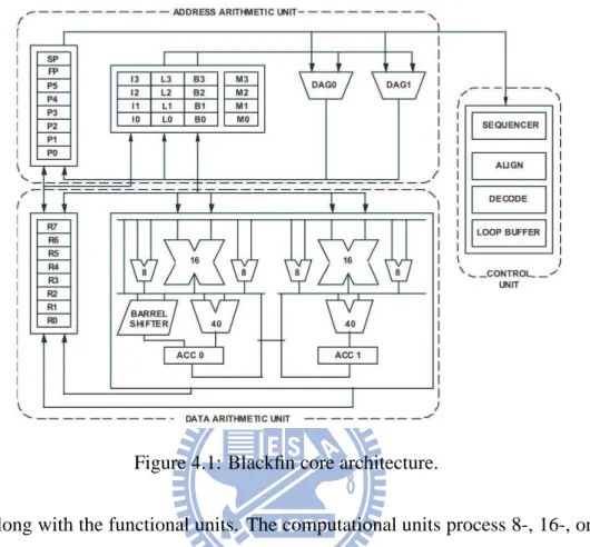
As shown in Figure 4.1, Blackfin core contains two 16-bit multipliers, two 40-bit ac-cumulators, two 40-bit arithmetic logic units (ALUs), four 8-bit video ALUs, and a 40-bit

Figure 4.1: Blackfin core architecture.

shifter, along with the functional units. The computational units process 8-, 16-, or 32-bit data from the register file. The compute register file contains eight 32-bit registers. When performing compute operations on 16-bit operand data, the register file operates as 16 inde-pendent 16-bit registers. All operands for compute operations come from the multiported register file and instruction constant fields. Each MAC can perform a 16- by 16-bit multi-ply per cycle, with accumulation to a 40-bit result. Signed and unsigned formats, rounding, and saturation are supported. The ALUs perform a traditional set of arithmetic and logical operations on 16-bit or 32-bit data. Many special instructions are included to accelerate various signal processing tasks. These include bit operations such as field extract and pop-ulation count, divide primitives, saturation and rounding, and sign/exponent detection. The set of video instructions includes byte alignment and packing operations, 16-bit and 8-bit adds with clipping, 8-bit average operations, and 8-bit subtract/absolute value/accumulate (SAA) operations. Also provided are the compare/select and vector search instructions.

CHAPTER 4. THE ARCHITECTURE OF ANALOG DEVICE BF561 23 For some instructions, two 16-bit ALU operations can be performed simultaneously on register pairs [4].

4.2

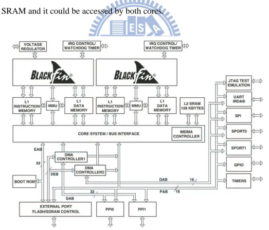
Blackfin ADSP-BF561

ADSP-BF561 is a member of Blackfin processor family of products targeting consumer multimedia applications. At the heart of this device are two independent enhanced Black-fin processor cores that offer high performance and low power consumption while retaining their ease-of-use and code-compatibility benefits. As shown in Figure 4.2, the two Blackfin cores are connected via buses, which is a complicated bus system. In addition to L1 instruc-tion SRAM and L1 data SRAM, there is a L2 SRAM works around half speed compared to L1 SRAM and it could be accessed by both cores.

4.2.1

Memory Hierarchy

Blackfin products support a modified Harvard architecture in combination with a hierar-chical memory structure shown in Figure 4.2. Generally speaking, a hierarhierar-chical memory architecture means there exists multi-level memory blocks and they run under different speeds from fast to slow. The memory block near the processor core often works on the highest speed and we call it Level 1 (L1) memory. Following the principle, the follower is L2, L3,... memory . A hierarchical memory structure is designed for cost and power effective.

Level 1 (L1) memory of Blackfin BF561 operates at the full processor speed with little or no latency. At the L1 level, the instruction memory holds instructions, the data memory holds data, and a dedicated scratchpad data memory stores stacks and the information of local variables.

L1 instruction SRAM consists of 32Kb SRAM, of which 16Kb can be configured as a four-way set-associate cache. If we configure it as a general instruction SRAM, it could be put not only instructions but also data. However, the data put in the instruction SRAM can be moved only by DMA and the core can not take the data from L1 instruction SRAM directly.

L1 data SRAM consists of two banks of 32Kb each. Half of each bank is always configured as SRAM while the other half can be configured as SRAM or a two-way set associate cache. In addition, there exists a block of 4Kb L1 scratchpad SRAM, which runs at the full speed but is only accessible as a data SRAM and cannot be configured as a cache memory.

For safe memory access, the Memory Management Unit (MMU) provides memory protection for individual tasks that may be operating on the core and can protect system registers from unintended access.

CHAPTER 4. THE ARCHITECTURE OF ANALOG DEVICE BF561 25 high speed SRAM access with somewhat longer latency than the L1 memory banks. The L2 memory is a unified instruction and data memory and can hold any mixture of code and data required by the system. It could be only configured as SRAM and cannot configured as a cache. On the other hand, it could be set to cache-able to data cache; this means it could be cached by the data cache. The total L2 SRAM size in BF561 is 128Kb.

The L1 instruction SRAM and data SRAM could be broken into 4Kb sub-banks, which can be accessed independently by the DMA and the core simultaneously.

External (off-chip) memory is accessed via the External Bus Interface Unit (EBIU). This 32-bit EBIU provides a gluless connection to as many as four banks of synchronous DRAM (SDRAM) and as many as four asynchronous memory devices including flash memory, EPROM, ROM, SRAM, and memory-mapped I/O devices. The PC133-complaint SDRAM controller can be programmed to interface to up to 512 MBs of SDRAM.

4.2.2

DMA Support

To see the architecture of ADSP-BF561, we could easily be attracted by the two DMA controllers. DMA is well known for efficient data movement, and exists not only in general CPUs but also in DSP processors. The advantage of the DMA devices in BF561 is that the buses are independent while connecting to internal L1 SRAM and L2 SRAM. This is special because most DMA devices in other processors are designed connecting to the main bus and share the bus access with processor cores and other devices connecting to the bus; that’s why we say “cycle stealing”. However, “cycle stealing” doesn’t exist in BF561 due to the independent DMA accesses; this means the utilization of DMA on BF561 could promote higher performance.

Since we say DMA accesses to internal L1, L2 SRAM could benefit from independent buses, the access to external SDRAM is all controlled by EBIU. This seems to make no big difference between core access and DMA access. However, the DMA access could be more efficient since it works under burst read/write.

For different purposes, the DMAs on BF561 can be categorized to three functions:

• Peripheral DMA (DMA): It is used to transfer data between peripheral devices and

internal L1, L2 SRAM

• Memory DMA (MDMA): It is used to transfer data between external SDRAM and

internal L1, L2 SRAM.

• Internal Memory DMA (IMDMA): It is used to transfer data between internal L1/L2

SRAM.

The Figures 4.3 shows the bus architectures of Blackfin BF561. we could see that there are independent buses connecting to L1 SRAM and L2 SRAM. If we can manipulate the accesses by the DMA devices and the cores overlapping, the performance can be promoted.

CHAPTER 4. THE ARCHITECTURE OF ANALOG DEVICE BF561 27

Implementation and Optimization

5.1

Experiment Environment Setup

There are several kinds of developing tools for us to develop our programs on BF561. The official integrated tool is Visual DSP++, which is a integrated developing environment (IDE) like ARM Developer Suite (ADS) in ARM-based environments. For more complex applications, they also developed a lightweight real-time kernel called VDK, which has many libraries for real-time applications for developers.

Instead of official tools we have another choice: GNU open-source project. In this project, we could use uClinux and GCC toolchains on Blackfin system; all the toolchains and uClinux are well supported by the community. uClinux is a lightweight version of Linux to support non-MMU processors.

We choose the open-source GNU project for our experimental environment for two rea-sons. First, an open-source environment is more proper for academic researches. Second, if we have Linux kernel support on BF561, we theoretically could transplant the codes from any other Linux-based platform and could exploit the library supports from Linux kernel; this is very convenient for us to develop our applications quickly since resources for Linux-based systems are easy to find on the Internet.

For dual-core BF561, uClinux could run on only one core or both cores. If uClinux runs on one core, the other core is treated as a device and could run programs through

CHAPTER 5. IMPLEMENTATION AND OPTIMIZATION 29 driver supports. In addition to running on one core, uClinux also could run on both cores; it is called “SMP-like” mode.

Why we say it’s “SMP-like” is that BF561 lacks of hardware cache coherency mecha-nism; a “real” SMP must have hardware supported cache coherency mechanism. Hence, cache coherency should be done by software mechanism when needed. This implicates three significant features [5]:

• caches must be in write-through mode,

• more overhead is introduced due to software coherency mechanism, and • all threads of a process are restricted to be executed on the same core.

Another problem is that the L1 SRAM owned by one core cannot be accessed directly from the other core so that L1 SRAM cannot be used in the kernel. Because it will cause kernel panic while the kernel threads running on one core try to access the kernel resources put in L1 SRAM of the other core. This would reduce the optimization potential because we cannot put critical system calls in the L1 SRAM to optimize Linux kernel. The devel-opments of user space applications also have to be taken care that the user process runs on a specific core if we try to put the data or instruction codes in the L1 SRAM.

We finally configure the uClinux as SMP-like mode because a full Linux supported environment gives us a consistent environment to develop applications. There are no needs to load programs to the other core by special drivers.

5.2

Software-based JPEG2000 Implementation and

Pro-filing

There are several projects working on open-source JPEG2000 codec. The most famous are Jasper [18] and OpenJPEG [20].

Jasper is developed and maintained by its main author, Michael Adams, who is affil-iated with the Digital Signal Processing Group (DSPG) in the Department of Electrical and Computer Engineering at the University of Victoria. It is developed for the imple-mentation of JPEG-2000 Part-1 standard (i.e., ISO/IEC 15444-1) and itself is a part of JPEG-2000 Part-5 standard (i.e., ISO/IEC 15444-5).

OpenJPEG implements not only Part-1 standard but also many other features like JP2 (JPEG2000) and MJ2 (Motion JPEG2000) file formats, JPEG2000 Interactive Protocol, and so on. It’s developed and maintained by Communications and Remote Sensing Lab, in the Universit catholique de Louvain (UCL).

With the comparison of two implementations, we choose OpenJPEG for our imple-mentation for two reasons: the source code is easy to trace and the code partition is clear.

Since the source code of OpenJPEG is well written and portable, it’s not too hard to port the code onto our platform. The uClinux is also easy to configure to SMP-like mode.

Figure 5.1 shows the execution time breakdown of JPEG2000 compression on BF561; the input image is a 640x480 color image taken from OpenJPEG official site and the pro-filing is subject to default setting: DWT level n=5, codeblock b= 64x64, lossless. We see that EBCOT Tier-1 and DWT dominate the JPEG2000 compression; the two components occupy 92% loading of the whole time. Our optimizations will be focused on these two parts because they are not only the hotspot of JPEG2000 compression but also potentially parallel parts.

5.3

Overview of JPEG2000 Optimizations on BF561

5.3.1

Data Locality Optimization

After we finish kernel and JPEG2000 porting to our BF561 environment, where do we start to optimize JPEG2000? As we know, image processing often divides an image (data) into several blocks and in concept the block is a 2-D array. However, memory accesses are

CHAPTER 5. IMPLEMENTATION AND OPTIMIZATION 31 EBCOT-Tier2 1% EBCOT-Tier1 71% DWT 21% pre-processing 7%

Figure 5.1: Execution time breakdown of JPEG2000 compression on the BF561 processor. practically 1-D; hence, it will have bad performance if we don’t carefully arrange the data in proper location. A big problem is the cache-miss problem. There are many researches in management of data locality in different design levels such as system-level, application-level or compiler application-level [26] [6] [1] [10].

As we discussed in Section 4.2.1, there are a L1 instruction SRAM, a data SRAM and a L2 SRAM companied with two DMA devices on the BF561 architecture. Now we focus on the data SRAM. Some of the L1 data SRAM can only be configured as general data SRAM rather than a cache, and therefore there is no cache-miss problem. The data SRAM works as fast as the core. This data SRAM is a precious resource for us to do the data optimization. For convenience, we simplify the term “general data SRAM” to be “data SRAM”.

The best scenario for the utilization of the L1 data SRAM is that we can put all data in it to achieve best performance. However, this often doesn’t happen due to the limited SRAM size. Hence, we only can move some of them into L1 SRAM; these may include

parts of the input data, output buffer, temporary data, constant data and so on.

On the other hand, we configure the parts that can be configured as a cache to be a cache because we know that this state-of-the-art mechanism could efficiently promote the performance without any software overhead. This configuration is a good choice for general utilization. However, the utilization of general SRAM depends on application developers. Hence, the utilization of SRAM is an emphasis of our optimization.

DMA is a technique designed for data moving and now almost exists in every modern CPU. There are also DMA devices in BF561 and the amount is two. Different to many other SOC and CPU designs, the two DMA devices in BF561 have independent buses and can access the SRAM in one sub-bank while Blackfin core is accessing another. Each of them has 16 channels, 4 of which could be used as Memory DMA (MDMA); it means that we could use them to move data among L1 SRAM, L2 SRAM, and external memory.

As a result, we can move data into L1 data SRAM by DMA before they are needed; then we move out these data after the processing is completed. Furthermore, it will be the best if the data moving can be overlapped with the accesses from processor cores.

The hotspot instruction codes also can be put in the instruction SRAM like we do in data. For the utilization of the instruction SRAM, GCC supports compiler intrinsics for us to put specific procedures into L1 instruction SRAM. For instance, we can simply use

attribute ((l1 text)) to put one procedure into the L1 instruction SRAM while we are

writing source code. It is put after the definition of the procedure we want to put in the L1 instruction SRAM. The following is an example to show how to use the intrinsic:

void foo(int a) attribute ((l1 text));

The function foo(int a) will be allocated in the L1 instruction SRAM and the linker will maintain the linking information for the call to foo.

CHAPTER 5. IMPLEMENTATION AND OPTIMIZATION 33

5.3.2

Utilization of Two Cores

After the discussion of SRAM, we talk about the two cores of BF561. If we could put parts of the calculating jobs onto the other core to be processed simultaneously, the per-formance will be promoted significantly. It is widely known that there are two ways to partition calculating jobs to multi-cores: task partition and data partition. Task partition means that many cores run different codes and the data are processed through these cores like a pipeline. Data partition means that many cores run the same code and the data are partitioned to these cores to be processed.

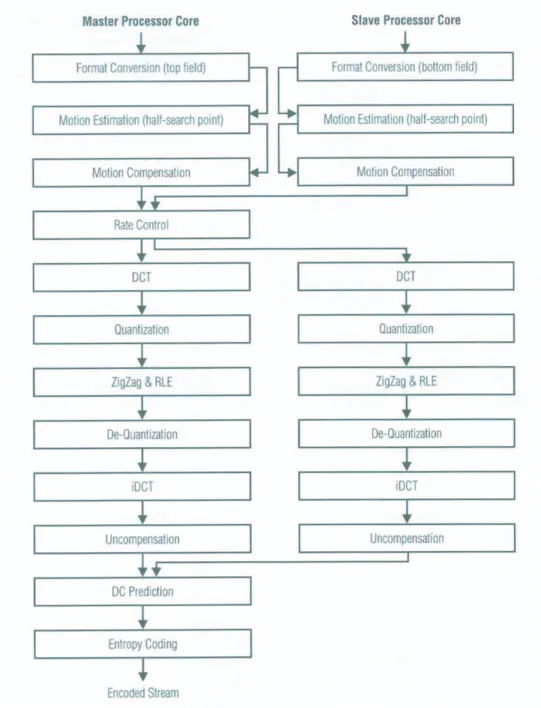
Similar to the principle, David J. Katz and Rick Gentile, the members of Analog De-vices’ Embedded Processor Application Group, use MPEG-2 as an example to show the two partition ways on Blackfin BF561 [14]. The first, as shown in Figure 5.2, is a

master-slave model; it’s similar to “data partition”. In this model, the coding process is mainly

controlled in master core and it spills some data to be processing in the other core. The advantage of this model is that we don’t need to change codes a lot; the development proce-dure is just similar to the development in one core. However, synchronization overhead is needed and the slave core would not be fully loaded. As the example shown in Figure 5.2, some components of the MPEG-2 compression are parallelized to both cores and some are not. Whether the components can be parallelized may depend on their algorithms. When running the unparalleled components, the slave core is in idle state. In addition, the syn-chronizations are needed after some components in order to make sure that the data for their next components are ready.

The other programming model is a pipelined model; it’s similar to “task partition” and some people call it “stream partition”. As shown in Figure 5.3, the compression procedure is divided into several sub-procedures and then these sub-procedures are dispatched to two cores. If the loading of two cores are balanced enough, the idle states happening in master-slave model don’t happen here. However, the whole developing procedure needs to be

CHAPTER 5. IMPLEMENTATION AND OPTIMIZATION 35

changed more and is not straightforward compared to which in master-slave model. To consider these two models we choose master-slave model for several reasons: first, it’s more scalable while the amount of hardware cores is changed; second, we could easily increase or decrease the loading of the slave core if we need to assign other jobs to the slave core; finally, JPEG2000 is hard to make balanced job partitions according to the profiling results we made, which are presented in Chapter 5.1.

5.4

Optimization of DWT

5.4.1

Data Locality Optimization

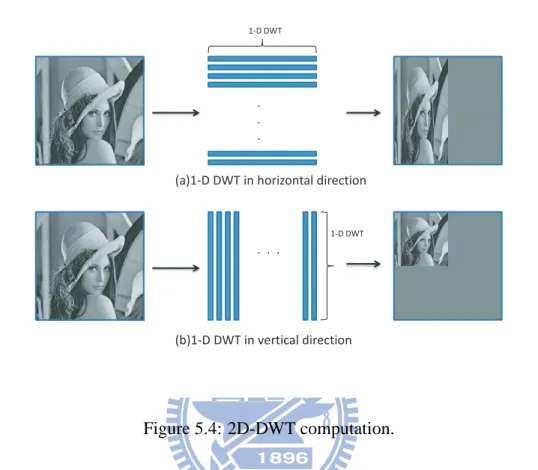
As we described in Section 3.2.2, JPEG2000 uses 2-D DWT computation to transform input image to high frequency and low frequency parts. The 2-D DWT computation is shown in Figure 5.4; we perform DWT calculation on the input image line by line in the horizontal and vertical direction, respectively.

Let’s take a close look at the dataflow of the DWT computation in Figure 5.5. Before we perform one-line DWT calculation, we need to move the line data into a buffer for the processor core to do the calculation. Thanks to the well designed (5,3) lifting-based DWT, it is a “in-place” calculation and we only need one buffer. In general case, processor itself can do the data moving well and data cache can cache the subsequent data for potential uses. Hence, it is easy to take the following data for processing in the high speed cache memory if our data are continuous in the memory; in image processing, it means that the data are from horizontal direction. However, this would suffer problems while reading from vertical direction. Furthermore, it is wasted if we just ask the processor core to do the data moving; it should focus on calculating jobs.

In general memory device, data are practically located and moved in 1-D mode even though the high-level description is in 2-D mode. For this reason, we change our view from 2-D to 1-D to see how data are moved into and out of the buffer. Figure 5.6(a) shows

CHAPTER 5. IMPLEMENTATION AND OPTIMIZATION 37 . . . . . . 1-D DWT

(a)1-D DWT in horizontal direction

(b)1-D DWT in vertical direction

1-D DWT

Figure 5.4: 2D-DWT computation.

the data moving scenario that how data are moved into the buffer from candidate line data in the horizontal direction. We could see that it is continuous reading while data are read to the buffer; this is the best model that cache can perform well.

Since the data is filled into the buffer, DWT computation can be performed to the data in this buffer. As discussed in Section 3.2.2, the DWT computation produces DWT co-efficients and the low frequency and high frequency coco-efficients are regularly interleaved. After DWT computation, while the data are moved back, we have to separate the low frequency coefficients and high frequency coefficients and put them back to the correct location. How data are moved back is shown in Figure 5.6(b). We see that high frequency and low frequency coefficients are centralized to the start and the middle of the original line data, respectively.

buffer

Blackfin core

sta!c void dwt_encode_1(int *a, int dn, int sn, int cas);

data flow data flow

Figure 5.5: Dataflow of DWT computation performed in one line.

in Figure 5.7(a), the data read from candidate line data are periodically separated by a fixed stride; this is bad for cache to handle. On the other hand, similar to the data restoration in the horizontal direction, we need to put the interleaved low frequency coefficients and high coefficients back to the correct location. Where the data should be put back is shown in Figure 5.7(b).

Through the observation and analysis, the actions of data moving, including data mov-ing into and out of the buffer, which are performed in the horizontal and vertical directions, can all be configured to be the jobs of DMA. The main reason about why DMA can per-form these data moving is that these data moving are regular. Suppose one “data moving” consists of moving of several data elements, if the elements of the source data are regularly placed in a fixed stride and their target location are also at a fixed stride, we call the data moving “regular” and it can be performed by DMA.

CHAPTER 5. IMPLEMENTATION AND OPTIMIZATION 39

buffer

candidate data in memory (a) Buffer fill from candidate data before DWT

………

(b) Data restora!on from buffer ………

…

buffer

…

: low frequency data : high frequency data

y03

x : the horizontal length of image y : the ver!cal length of image

…… ……

……

candidate data in memory

Figure 5.6: The data moving flow in a horizontal line.

As a result, we can use DMA to move data into and out of the buffer and we just put the buffer into the L1 data SRAM to be accessed in high speed clock rates. The dataflows before and after our optimization are illustrated in Figure 5.8. We add the cache into the figure to show the specialty of our optimization. We can see that our optimization bypass the cache mechanism.

Because of the frequent invocations of DMA operations, a low latency system call to configure DMA controllers is essential. For this reason, we write a lightweight system call instead of standard Linux I/O control driver and put it in the L1 instruction SRAM. In addition, thanks to the problem that L1 instruction SRAM cannot be accessed by the other core, the DMA system call is cloned to the L1 instruction SRAM of both cores in oder to be accessed from both cores.

buffer

y

(a) Buffer fill from candidate data before DWT ………

(b) Date restora"on from buffer

……… …

buffer

…

: low frequency data : high frequency data

y

y y

y+z03

y

x : the horizontal length of image y : the ver"cal length of image

……

……

…… candidate data in memory

candidate data in memory … … …

… …

Figure 5.7: The data moving flow in a vertical line.

5.4.2

Utilization of Two Cores

5.4.2.1 Data Partition

After the discussion of optimization using DMA and internal SRAM, we discuss how to partition the calculation jobs to the other core. As we mentioned in Section 5.3, we use data partition to spread the half of the data to the other core to speed up the calculation. The fact that L1 SRAM cannot be accessed by the other core would still be a problem at this moment. This enforces us to bind the user process to one of two cores; this means that we should enforce the Linux kernel to schedule the process on only one core. This could be achieved by system call int sched setaffinity(pid t pid, unsigned int cpusetsize,cpu set t

*mask). Another problem is that on BF561 a thread can only run on one core with its

process due to the lack of hardware cache coherency. As a result, we have to fork a new process and bind it to the other core to help us share calculations. The new process is

CHAPTER 5. IMPLEMENTATION AND OPTIMIZATION 41

buffer

Blackfin core

sta"c void dwt_encode_1(int *a, int dn, int sn, int cas);

dataflow dataflow

cache _buffer

Blackfin core

sta"c void dwt_encode_1(int *a, int dn, int sn, int cas);

DMA data moving

L1 data SRAM

DMA data moving

cache

(a) (b) L1 data SRAM

Figure 5.8: Dataflow of DWT computation performed in one line: (a) before data locality optimization (b) after data locality optimization.

generated after performing vfork() and exec() families.

The only parameter needed to pass to the new process is the address of the tile address (which is the start address of the image in our scenario); it is put in shared L2 SRAM. L2 SRAM is now used as a shared memory for us to communicate between two cores. As we discussed, the DWT performed in each line is independent; hence, we divide the line data of the same direction at the same level into two groups: half front parts and half back parts, and perform DWT on different cores as shown in Figure 5.9. Until the computations of dispatched jobs at both cores are finished, the next stage, which may refer to different direction or the next level, are not allowed to start; this means that the synchronization is needed here to make sure both cores finish their jobs. We use shared variables for synchronization; they are placed in shared L2 SRAM.

However, we find that the data partition to two cores is inefficient. The main reason is that the loading of data transfer is heavy—more discussions will be given in Section 6.1.

. . . 1-D DWT vfork() sync . . . 1-D DWT sync core A core B . . . . . .

Figure 5.9: The data partition to two cores.

Hence, we propose another method to partition jobs of DWT. This is discussed in the following subsection.

5.4.2.2 Task Partition

Due to the heave loading in data transfer, we try to partition DWT computations in another way (we name two cores as CoreA and CoreB for discussion); we try to partition jobs between memory transfers and DWT computations themselves. We ask CoreA to focus on DMA control; CoreA is responsible to control DMA to move the data into L1 data SRAM of CoreB, and CoreB focuses on the DWT computation but needn’t to care about the data transfer. As discussed in Section 4.2.1, the data transfer using DMA control and core access could be overlapped; this makes the memory/calculation partition possible. The scenario can be shown in Figure 5.10. We finally sum up our optimizations with Algorithm 1 and Algorithm 2, which show what CoreA and CoreB do, respectively. As we discussed above,

CHAPTER 5. IMPLEMENTATION AND OPTIMIZATION 43 CoreA moves data and CoreB does the computations. For the cooperations of two cores, we set a synchronization machanism to make sure that each DWT computation starts after the completion of moving out of the old data and moving in of the new data. The experimental results presented in Section 6.1 shows that the performance of task partition is better than that of data partition for the DWT process.

Core B Core A External memory control data transfer data transfer L1 data SRAM bank 1 L1 data SRAM bank 2

Algorithm 1: DWT: The workload of CoreA

Input: three components of the input image: Y, U, V Output: DWT coefficients

for each component of the input image do for each resolution level do

for each sub-band do

for each 2 vertical lines of the input image do

move the old data out;

move the first line data into Bank-1 of data SRAM of CoreB; sync 1; //notify CoreB data in Bank-1 are ready;

move the old data out;

move the second line data into Bank-2 of data SRAM of CoreB sync 2; //notify CoreB data in Bank-2 are ready;

end

for each 2 horizontal lines of the input image do

move the old data out;

move the first line data into Bank-1 of data SRAM of CoreB sync 1;//notify CoreB data in Bank-1 are ready;

move the old data out;

move the second line data into Bank-2 of data SRAM of CoreB sync 2;//notify CoreB data in Bank-2 are ready;

end end end end

Algorithm 2: DWT: The workload of CoreB

Input: three components of the input image: Y, U, V Output: DWT coefficients

sync 1;//wait Bank-1 data ready;

DWT 1D(bank-1);//perform DWT put in Bank-1; sync 2;//wait Bank-2 data ready;