GRAVITATIONAL STRESSES IN ANISOTROPIC RIDGES AND VALLEYS WITH SMALL SLOPES

JOURNAL OF GEOPHYSICAL RESEARCH, VOL. 97, NO. B3, PAGES 3325-3336, MARCH 10, 1992

Gravitational Stresses in Anisotropic Ridges and Valleys

With Small Slopes

JVH JONG LIAO

National Chiao Tung University, Department of Civil Engineering, Hsinchu, Taiwan

WILLIAM Z. SAVAGE

U.S. Geological Survey, Denver Federal Center, Denver, Colorado

BERNARD AMADEI

University of Colorado, Department of Civil Engineering, Boulder, Colorado

We present an approximate analytical solution for the effects of topography on near-surface gravity-induced stresses in symmetric anisotropic ridges and valleys. The solution can be used for laterally constrained ridges and valleys consisting of isotropic, transversely isotropic, or orthotropic rock with horizontal or vertical layers. A parametric study on the effect of anisotropy type and degree of rock anisotropy on gravity-induced stresses is presented. The magnitude of the predicted stresses is of the order of the characteristic stress pgH, where H is the height of the ridge or depth of the valley. The approximate solution is limited to ridges and valleys with small slopes not exceeding 10%.

INTRODUCTION

Stresses induced by gravity in rock masses are often predicted using analytical solutions that model rock as a homogeneous, linear elastic, and isotropic continuum. The gravity-induced stress field is commonly described as result- ing from a vertical component due to the weight of overlying rock and a horizontal component which is v/(1 - v) times the vertical component, where v is the rock Poisson's ratio. The horizontal component is a consequence of assuming that horizontal displacements are zero, the condition of lateral constraint. However, measured horizontal stresses often differ from those predicted by the lateral constraint condi-

tion. These differences have been attributed to the effects of tectonic, residual, and thermal stresses, erosion, lateral straining, anisotropy, and topography [Jaeger and Cook, 1976; McGarr and Gay, 1978; McGarr, 1988]. The effects of rock mass anisotropy and topography on gravity-induced stresses in a laterally constrained elastic half-space are considered in this paper.

Because of the processes that form rocks or because of later processes that move and deform them, many rocks are anisotropic, which means that their mechanical properties vary with direction. This variation is often related to the existence of well-defined rock fabric elements in the form of bedding, stratification, layering, schistosity planes, foliation, fissuring, or jointing. Mechanical anisotropy is generally a characteristic of foliated metamorphic rocks (schists, slates, gneisses, phyllites), stratified sedimentary rocks (shales, sandstones, limestones, coals), and rocks cut by one or several regular, closely spaced joint sets. All of these rocks display clear evidence of physical discontinuities and show one or several apparent directions of symmetry, and they are

Copyright 1992 by the American Geophysical Union. Paper number 91 JB02960.

0148-0227/92/91 JB-02960505.00

usually mechanically anisotropic [Amadei et al., 1987]. For anisotropic rock masses the relation v/(1 - v) between vertical and horizontal stress components is no longer appli- cable. Expressions for the relationship between horizontal and vertical gravity-induced stresses in rocks with horizontal or vertical anisotropy are given by Amadei et al. [1987, 1988] and Amadei and Savage [1985]. These analytical solutions for gravity-induced stresses are limited in only being appli- cable to rock masses with flat ground surfaces. The effect of topography has been addressed by Ter-Martirosyan et al. [1974], Savage et al. [1985], Savage and Swolfs [1986], and McTigue and Mei [1981, 1987]. These solutions, however, consider the rock to be isotropic.

In this paper an approximate analytical solution is given for gravity-induced elastic stresses in symmetric mechani- cally anisotropic ridges and valleys. In what follows, the elastic properties of anisotropic rocks are briefly described, the derivation of the approximate analytical solution is given, parametric studies for some examples are illustrated,

and the limitations of this solution are discussed.

ROCK ANISOTROPY

The directional character of the linear elastic properties of anisotropic rocks can be assessed by testing specimens in the field or in the laboratory [Amadei, 1983; Wei and Hudson, 1988] and analyzing the results by the theory of linear elasticity for anisotropic media. A general form for the constitutive relation of an anisotropic elastic medium in an arbitrary x', y', z' coordinate system can be written in matrix form as

=

where (e) and (t r) are (6 x 1) column matrix representations of the strain and stress tensors, respectively, in the x', y', z' coordinate system and (C) is a (6 x 6) compliance matrix

3326 LIAO ET AL.' GRAVITATIONAL STRESSES IN RIDGES AND VALLEYS

with components

cij (i, j = 1 -• 6). Equation

(1) is also

known as the generalized Hooke's law, and matrix (C) has 21 distinct components if a strain energy function is assumed to exist in the medium. This type of anisotropy is called general anisotropy [Lekhnitskii, 1977].

In most practical cases, anisotropic rocks can be modeled as orthotropic or transversely isotropic materials in a coor- dinate system attached to their apparent structure or direc- tion of symmetry. Orthotropy implies that three orthogonal planes of elastic symmetry exist at each point in the rock and that these planes have the same orientation throughout the rock. (A plane of elastic symmetry exists at a point if the compliances of the anisotropic medium have the same values for every pair of coordinate systems that are the reflected images of one another with respect to the plane.) Transverse isotropy implies that at each point in the rock, there is an axis of symmetry of rotation and the rock has isotropic properties in a plane normal to this axis. This plane is called the plane of transverse isotropy [Lekhnitskii, 1977].

For a material that is orthotropic in an x', y', z' coordi- nate system, i.e., with planes of symmetry normal to the coordinate axes, equation (1) can be written as follows:

i 1,21 1,31

o o

i'

ø ø0

=

1

(2)

y'z'

0

0

0

-'- 0

•,z,

0

0

0

--

•

0 0 0 0 G•

where El, E2, E3 are Young's moduli in the x', y', z' directions, respectNely, and G 12, G23, G 13 are shear moduli in planes parallel to the x'y', y'z', and x'z' coordinate planes, respectNely. Thus the shear compliance 1/G 12 char-

acterizes

the shear

strain, 7•?', response

to the shear

stress

r•?,. The Poisson's

ratio pq characterizes

the compressNe

or tensile strain response in the j direction to a uni•ial tensile or compressNe stress acting in the i direction. For example, Pl2 characterizes the extensile strain response in the y' direction to a compressNe stress acting in the x'

direction.

Of the 12 elastic constants entering into equation (2), only nine are independent, owing to the following symmetw conditions [Lekhnitskii, 1977]:

1,12 1,21 1,13 1,31 1,23 1,32

E1

- E2 E1

- E

3 E2

- E3.

(3)

Typical values of the nine elastic constants

El, E2, E3, 1,21,

1,31, 1,32, G12, G13, and G23 for those different rock types are given by Gerrard [1975] and Amadei et al. [1987].

For a material that is transversely isotropic, only five independent elastic constants are needed to describe its deformational response. In this paper these constants will be called E, E', 1,, v', and G' and are defined as follows:

1. Constants E, E' are Young's moduli in the plane of transverse isotropy and in a direction normal to it, respec- tively.

2. Constants 1,, 1,' are Poisson's ratios characterizing the lateral strain response in the plane of transverse isotropy to a stress acting parallel or normal to it, respectively.

3. Constant G' is the shear modulus in planes normal to the plane of transverse isotropy.

Equation (2) also applies to a material that is transversely isotropic in one of the three coordinate planes of the x', y', z' coordinate system. The elastic parameters entering into this equation can be expressed in terms of the five constants defined above. For example, if there is a plane of transverse isotropy parallel to the y'z' coordinate plane, we have

E 3 = E 2 = E Ei=E' 1'32 = 1,23 = 1, (4) ! 1,12 = 1,13 = 1, G12 = G13 = G'.

In addition, G23 = G = E/[2(1 + 1,)], and using equation (3),

E

v31=

v21=

v' E"

(5)

The transverse isotropy formulation can be used to char- acterize the deformability of rocks such as schist, slate, gneiss, phyllite, siltstone, mudstone, sandstone, shale, and basalt. For such rocks the plane of transverse isotropy is

assumed

to be parallel to foliation, schistosity,

or bedding

planes. Elastic constants for rocks modeled as transversely isotropic materials are given by Gerrard [1975] and Amadei et al. [1987].

If the rock is isotropic, only two elastic constants are needed to describe its deformability: E = E', v = v', and G = G' = E/[2(1 + 1,)].

Except for isotropic symmetry, the constitutive equation for an anisotropic medium depends on the choice of coordi- nate system. In the x', y', z' coordinate system, the constitutive equation is defined in equation (1). In another x, y, z coordinate system, the constitutive equation can be

expressed as

( • )xy• = (A)( rr)xy

z,

(6)

or

•x all a12 a13 a14 a15 a16

a21 a22 a23 a24 a25 a26

a31 a32 a33 a34 a35 a36 a41 a42 a43 a44 a45 a46 as1 a52 a53 a54 a55 a56

a61 a62 a63 a64 a65 a66

LIAO ET AL ß GRAVITATIONAL STRESSES IN RIDGES AND VALLEYS 3327

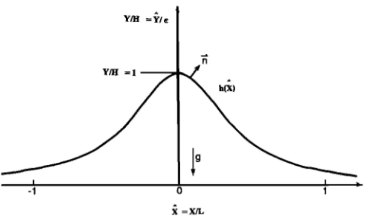
Y/H =•'/e

Fig. 1. Isolated symmetric ridge.

where (e)xy

z and (O')xy

z are the (6 x 1) matrix representa-

tions of the strain and stress tensors in the x, y, z coordinate system. As was shown by Lekhnitskii [1977], the compo-

nents aij = aji(i, j = 1, 6) of the compliance

matrix (A)

depend

on the components

cij(i, j = 1, 6) of matrix (C) in

equation (1) and the orientation of the x', y', z' axes with respect to the x, y, z coordinate system.

The relationships

between

the elastic

compliances

a ij and

the elastic

compliances

c ij [Lekhnitskii,

1977]

are

(C) = (Q)(A)(Q) t

(8)

where (Q) is a coordinate transformation matrix with com-

ponents

q ii given by Lekhnitskii

[1977].

Equation (8) can also be solved for (A) in terms of (C) as

(A) = (R)t(C)(R)

(9)

with (R) t = (Q)-I and (R) -1 = (Q)t.

GRAVITATIONAL STRESSES IN ANISOTROPIC RIDGES AND VALLEYS WITH SMALL SLOPES

Because mathematical difficulties appear to preclude an exact analytical solution for gravitational stresses in an anisotropic ridge or valley, a perturbation scheme similar to that given by McTigue and Mei [1981] is used to derive an approximate solution. The approximate dimensionless

stresses

are presented

with an error

of the order

of e 2, where

e is a characteristic slope of the ridge or valley. Since this approximate solution is sufficiently accurate only when e is very small, it will be shown that this solution is limited to predicting gravitational stresses in the near surface of aniso- tropic ridges or valleys that have •,•p

Assumptions of the Problem

The following assumptions (also used by McTigue and Mei [1981 ]) are made in the solution for gravitational stresses in an anisotropic ridge or valley:

1. The ridge is assumed to be symmetric with a shape like that shown in Figure 1. H, L, and e = H/L << 1 are defined as the characteristic height, length, and slope, re- spectively. Also, the dimensionless coordinates 2 and p are normalized by L (2 = x/L and p = y/L), and the dimen- sionless surface configuration h(2) is normalized by H. The geometry of the ridge can be expressed as

y =

Y

Y

(c) (d)

Fig. 2. (a) Orthotropic and (b, c, d) transversely isotropic rock masses with horizontal and vertical planes of elastic symmetry parallel to the coordinate axes.

or

y = h(2)H (11)

Equations (10) and (11) can also represent the geometry of a symmetric valley when H represents the depth of the valley. 2. Transversely isotropic and orthotropic rock masses with horizontal and vertical planes of elastic symmetry parallel to the coordinate axes as shown in Figure 2 are considered. This is a plane problem with no traction over the boundary and gravity acting in the -y direction.

3. Dimensionless stress components are used where

&x = Crx/pgH,

O'y

--- Cry/pgH,

&z = crz/pgH,

and •'xy : rxy/

p#H, where p is density and # is gravitational acceleration.

Solution for Gravitational Stresses in Anisotropic Ridges and Valleys With Small Slopes

As was shown by Amadei et al. [1987], gravity-induced stresses in a flat-lying anisotropic rock mass with horizontal and vertical planes of elastic symmetry can be predicted by

cr x - pgy

cr z- -al3 •+ a23 pgy (12) a33 /•11

O'y = pgy

r xy -- 0

where tgij = aij - (ai3aj3)/a33 and aij are the elastic

compliances of the rock mass in the x, y, z coordinate system attached to the half-space. The stress field defined in equation (12) was derived assuming no lateral displacements in the xz plane.

Because of the existence of topography, a dimensionless stress function F(2, p) is used here to express how stresses depart from the gravitational stresses in a flat-lying anisotro- pic rock mass. When topography exists, then, the dimen-

3328 LIAO ET AL.' GRAVITATIONAL STRESSES IN RIDGES AND VALLEYS

sionless

stress

components

in the half-space

bounded

by the

topography

can be expressed

as

]• 12 9 0 2F

/311

E 0• 2

•

02F

&y = -+

•r z =

(a13•r

x + a23•'y)

Equation

(13) satisfies

the equilibrium

equations

and the

compatibility

equations

in the lower half-space.

As was

proposed

by Lekhnitskii

[1939],

F(œ, •) is a solution

of the

equation

04F

04F

04F

• + (2/3

12

+ •66)

05720y2

+ ]• 11

0y4

/•22

0574

Second, the dimensionless

stress function F(57, •) is as-

sumed to be a power series in the small parameter e, e.g.,

F = F © + eF (1) + O(e 2)

Substituting

equation

(18) into equation

(15), the boundary

conditions

are rewritten

with an error

of the order

of e2 as

Oh

qxy--

EO'x

•-•

4-

O(E

2)

Oh

= ^ •+

O(e 2)

•'y E

r xy

057

(20)

(at :9 = eh). Substituting

equation

(13) into equation

(20) and

expanding

about :9 = 0, equation

(20) becomes

02F(57,

O)

03F(57,

O)

•12 Oh

+eh =e h

with the boundary conditions

&x

cos

(n,

57)

+ •'xy

COS

(n,

:9)=

0

0572

?xy

COS

(n, 57)

+ •ry COS

(n, :•)= 0

at p = eh(57),

where

n is the outward

normal

to the surface

of the ridge. Note that in the expression

of &z in (13), the

stress

function

F(57, •) is assumed

to induce

no strain in the

z direction only (plane strain analysis).

To solve equation

(14) with the traction-free

boundary

condition

(equation

(15)), a pertubation

scheme

like that of

•22

McTigue and Mei [1981] is used.

First, to define the direction cosines

on the boundary

surface,

• = eh(57),

recall that the unit normal (n) of a

surface,

f(x, y, z), is given as [Kreyszig, 1983]

grad f

n = •

= cos (n, x)i + cos (n, y)j + cos (n, z)k

Igrad fl

(16) and

where i, j, and k are the unit vectors

in the x, y, and z

coordinate

directions,

respectively,

and grad = V = (O/Ox)i

+ (O/Oy)j 4- (O/Oz)k.

Then for the dimensionless

surface

configuration, h(57), (17) (18) v(y -

Oh

( 1 2

057

2

1 2 e

1 2(Ohl

2

2

+"'

O

2F(57,

0)

O

3F(57,

0)

Oh O

2F(57,

0)

057 oy 2

+ O(e 2)

Oh O

2F(57,

0)

= -h- e

+ O(e 2)

Finally,

substituting

equation

(19) into equations

(14) and

(21) and collecting

like powers of e result in the two

following boundary value problems:

0 4F(ø)

0 4F(ø)

0 4F(ø)

0574

+ (2/•12

+ •66)

05720p2

+ •11 0p4

O

4F(1)

O

4F(1)

O

4F(1)

0574

+ (2/312

+ •66)

05720p2

+ /311

0p4

_ Oh

O

( O

2F(ø)

1

O2F(1)

/•

12

h

h

p = 0

c3570•

-- /3

ll 057 057 c]•

2 •

O2F

057

2 = 057

(1) O

(O2F(ø)

h 0570:91

1

=0 y=0.

Equation

(22) corresponds

to the problem

of a distributed

normal traction acting on the flat surface of a half-space,

whereas

equation

(23) corresponds

to the problem of a

distributed shear traction acting on the flat surface of a

half-space.

These

two boundary

value

problems

are solved

using

the complex

variable

method

given by Lekhnitskii

[1939] for stresses

in anisotropic

elastic half-spaces.

By

superposing

equations

(22) and (23), the traction-free

bound-

ary problem

of interest

can be approximated

to O(e).

The components

of the dimensionless

gravitational

LIAO ET AL.' GRAVITATIONAL STRESSES IN RIDGES AND VALLEYS 3329

stresses in the near-surface region can be obtained by expanding the stresses (equation (13)) about • = 0 and introducing equation (18). Thus

/312

y 02F(ø)(5:,

0)

02F(1)(œ,

0)

O

3F(ø)(œ,

0)

-3-

)

-3-

0(œ 2)

0y 3

h + O(g 2)

^ [ 1/3120

rxy

= e 2 1311

0œ

(h2)

+ •-• h

O

2F(ø)(œ,

0))

O

3F(ø)(œ,

0)

-- )

+ O(e 2)

05:0)

2

For known values of [02F(ø)(5:,

0)]/O) 2, [02F(1)(5:,

0)]/

0) 2 [03F(ø)(œ 0)]/0) 3 and [03F(ø)(œ 0)]/0œ0)

2 the

approximate gravitational stresses, with an error of the order

of O(e2) in the anisotropic

ridge,

can be predicted.

Consider a symmetrical ridge or valley for which h in equation (10) is such that

2

a

= (25)

a 2 + 5:2

The plus and minus signs correspond to a ridge and valley, respectively. The geometry of the ridge and valley is defined in an 5:/e = x/H, p/e -- y/H coordinate system by two parameters: a and e. The slope of the ridge or valley at the

inflection

points

is equal

to (3X/•/8)(e/a), and

the inflection

points

are located

at x/H = +a/eX/-•

and

y/H - 0.75 for a

ridge and -0.75 for a valley.

Substituting equation (25) into equations (22) and (23) and solving the resulting two boundary value problems by the approach described by Lekhnitskii [1939] give for a symmet- ric ridge

02F(ø)(5:,

0) a2A1 + aB15:

5:2

+ a 2

O

3F(ø)(5:,

0)

Op

3

= -{2a 25:[A

1 (a 1

+ a 2) -B 1 (/• 1

+/• 2)]

+ a(5:2-a2)[Al(Igl+lg2)+Bl(al+a2)]}[(5:2+a2)2]

-1

O

3F(ø)(5:,

0)

2a2A15:

+ aBl(5: 2- a 2)

05:0)2

(5:2

+ a2)2

O

2F(1)(5:,

0)

(a 1 + a 2)(A2 A3-B2B3 )-(fi 1 + 132) (A2B3 +A3B2)

8(5:2+a2)

3

and thus

/•12 ) aA1 + B15: &x-

1311

e

5:2

+ a 2

(a 1 +a 2)(A2A3-B2B3)-(fi l + fi2)(A2B3 +A3B2) -- E

8(5:2

+ a2) 3

- )a{2as:[Al(a 1+ a 2)-B1 (/31+

]32)]

+(5:

2-a 2)

ß

[Al(/gl+/32)+Bl(al+a2)]}[(5:2

+ a2)2]-l+o(e 2)

•'y --

2•

+ O(e 2)

/•12 2a45:

fill ( a2 + 5:2)3

+

a3(,3B15:2

+

4aA15:-

a2B1)

aBl(5: 2- a 2) + 2a2A15:

+

(a

2 + 5:2)

2

) + O(e

2)

&z =

(a 13•-x

+ a23•'y

)

a33

where a•, a 2 and/3•, ]•2 are the real and imaginary parts of /x•, /x2, respectively, /xl, /x 2 and their conjugates are the

/.1,4

_ 2/3•6/X3

=

roots

of/3•1

+ (2/312

+ J•66)#

'2 - 2f126/x

+ J•22

as: + 8Bla 2 + 4Alas:

B3 6 /• 12 2

2

fill

For a valley the dimensionless gravitational stresses can be obtained by changing the sign of the second and fourth

terms

in &x and the sign

of the second

term in &y and •xy in

equation (27). Note that the vertical dimensionless stress,

6-y, in equation

(27) is independent

of the elastic

properties

of the medium for both ridges and valleys.

When the ridge or valley is composed of isotropic rock, C•l = 6•2 -- O, J•l -' J•2 -- 1,A1 = -1,B1 = Oand-1312/1311 = v/1 - v (v is the rock Poisson's ratio). Then, equation (27) reduces to

v .,9

a 2

2 - 3v a(3a 4 - 6a25:2

- 5:4)

1 - v e a 2 + 5:2

+ e 2- 2v

(a

2 + 5:2)3

2a(a2 - 5:2

)

(a

2

+ 5:2)2

) + O(e2)

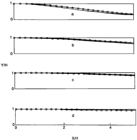
3330 LIAO ET AL.' GRAVITATIONAL STRESSES IN RIDGES AND VALLEYS Y/H 1 0 0 t I 0 2 4 X/H

Fig. 3. Comparisons of the topographic surface for ridges of (a) 19.5%, (b) 9.75%, (c) 6.5%, and (d) 3.25% slope at the inflection point. Squares predicted by equations (30) and (31). Solid line predicted by equation (29).

a 2

y

Y

(a/e) 2

a

2 + œ2

+ O(s2)

(28b)

H s (a/s)

2 + (œ/s)

2

2 - 3 v

4a 4.•

2a 2ϥ

•xy = e

_{2 - 2v (a}

_{2 + .•2)3}

_{- (a}

_{2 + &2)2}

_{+ O(t•}

2)

(28c)

•'z = P( •'x -3-

t3'y)

(28d)

Equations (28) are the same as the equations given by McTigue and Mei [1981], who used the Fourier transform method to solve the boundary value problems defined by equations (22) and (23).

DISCUSSION OF THE APPROXIMATE SOLUTION

Gravitational stresses in an elastically anisotropic ridge or valley can be approximated to O(s) by equation (27). The accuracy of the approximate analytical solution depends on the value of the characteristic slope s and the geometric parameter a for the ridge or valley. To estimate the accuracy of the approximate solution (equation (27)), the approximate gravitational stresses in an isotropic ridge (equation (28)) are compared with those determined with the exact solution for the isotropic ridge of Savage et al. [1985].

For the purpose of comparing the two solutions, the dimensionless expressions of the surface topography in equations (10) and (25) are normalized by the characteristic height H. Then the surface topography can be expressed as

(29)

Savage et al. [1985] define the surface topography by the following equation: x u a'u • (30) b b u2+a '2 and 12 (31) b //2 + a '2

where b is the ridge height. Note that in equations (30) and (31), a' has been used instead of a (as in the original equation of Savage et al. [1985]) in order to distinguish it from a in equation (29).

Figure 3 shows the topography of a ridge predicted by equation (29) for a - 1/3, 2/3, 1, 2 and e - 0.1 which corresponds to slopes at the ridge inflection points of 19.5%, 9.75%, 6.5%, and 3.25%, respectively. Also shown in Figure 3 is the topography of a ridge predicted by equations (30) and (31) with a' - 3.333, 6.666, 10, and 20, respectively. These values of a' were selected to make the surface topography predicted by equation (29) similar to that predicted by equations (30) and (31).

The accuracy of the approximate solution for stresses at a point in the isotropic ridge can be defined as follows:

LIAO ET AL.: GRAVITATIONAL STRESSES IN RIDGES AND VALLEYS 3331 1.0 1.0 0.2 -0.6 -1.4 -2.2 Y/H -3.0 0.0 0.8 1.6 2.4 3.2 4.0 0.0 0.8 1.6 2.4 3.2 4.0 (a) (b) 1.0 1.0 0.2 -1.4 -2.2 -30 00 08 16 24 32 40 (C) X/H

i

i '"'•r..-• i

Fig. 4. Contours of the error in the approximation solution for &x for isotropic ridges with (a) 19.5%, (b) 9.75%, (c) 6.5%, and (d) 3.25% slopes at the ridge inflection points.

ERR - x 100% (32)

Se

where S e and S a are the exact and approximate dimension- less gravitational stresses, respectively. When ERR - 0, the approximate solution coincides with the exact solution.

Figure 4 shows the contours of the error in the dimension- less horizontal stress component &x for the four isotropic ridges shown in Figure 3. Figure 4 shows that the error increases as the value of the parameter a decreases (slope increases) and as the dimensionless depth (y/b) increases. If a 10% error is adopted, the approximate solution can be applied to predict the gravitational stresses (1) near the surface for ridges with 19.5% slope, (2) down to •9/s = y/b = 0.6 along the axial plane (x/b - 0) and to greater depths away from the axial plane for ridges with 9.75% slope, (3)

•own to p/s = y/b = 0 along the axial plane and to greater

depths as x/b increases for ridges with 6.5% slope, and (4) in the full domain of Figure 4d for ridges with 3.25% slope.

Similar studies that we conducted of the error in the

dimensionless

vertical stress &y for the isotropic ridges

shown in Figure 3 show that the approximate solution can be reasonably used to predict the vertical stress in ridges with slopes less than 10%. Other studies comparing the exact and

approximate

solutions

for &x and &y in symmetric

isotropic

valleys show that the approximate solution can be used to

calculate the gravitational stresses in valleys with 10% slope at depths down to •/• = y/b -- -3.

Of course, comparison between the exact and approxi- mate solutions is possible only in the isotropic case. A large anisotropy may invalidate the conclusion that the approxi- mate solution is limited to ridges and valleys with small slopes not exceeding 10%.

ILLUSTRATIVE EXAMPLES

We present two examples to investigate the distribution of gravitational stresses in anisotropic ridges and valleys: (1) ridges with 6.5% slope at the inflection points of the ridge (a = 1 and e = 0.1) and (2) valleys with 6.5% and 9.75% (a = 2/3 and e = 0.1) slopes at the inflection points of the valley. The ridges and valleys are considered to consist of different isotropic, transversely isotropic, and orthotropic rocks. The effect of the rock's elastic properties and the orientation of the elastic anisotropy on the gravitational stresses is presented.

The gravitational stresses in anisotropic ridges and valleys are approximated by equation (27), which shows that the

dimensionless

vertical

stress

&y is independent

of the rock's

elastic properties. On the other hand, the other stress

components,

&x, &z, and '?xy,

depend

on the elastic

proper-

3332 LIAO ET AL.' GRAVITATIONAL STRESSES IN RIDGES AND VALLEYS Y/tl 1.0 1.0 1

0.6

0.6

0

•

-1

0.2

0.2

0 ••____•11

-1.0 -0.6 -0.2

(a)

0.2 0.6 1.0 -1.0 -0.6 -0.2(b)

0.2 0.6 1.0 -1.0 -0.6 -0.2(c)

0.2 0.6 1 0

0.6

0.6

.

'

I "'••

-1

.o

.o o.o •.o -•.o o.o •.o

(h) (i)

X/L

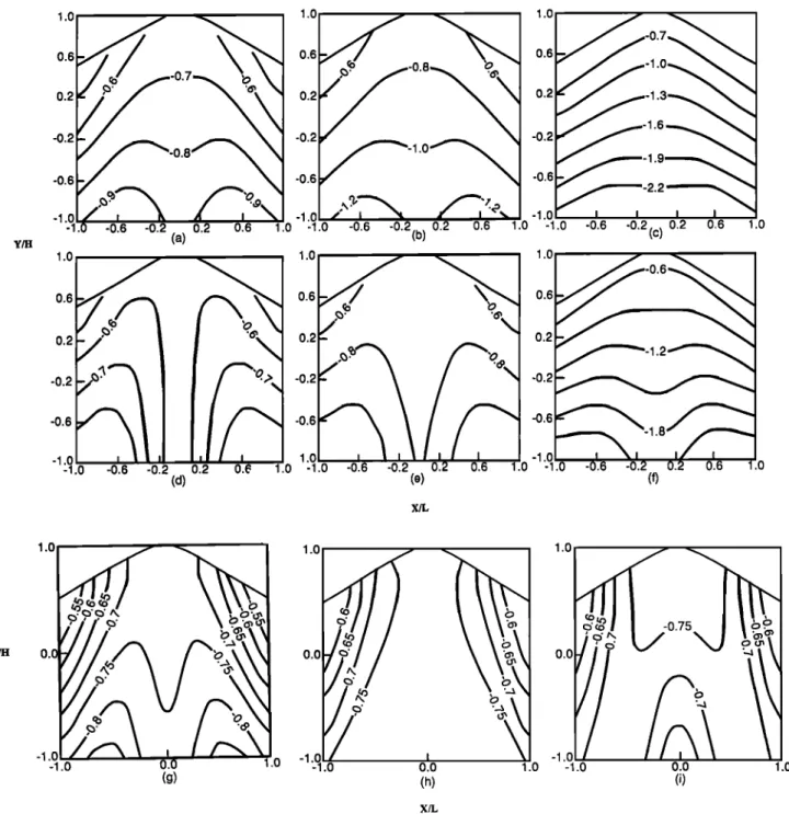
Fig. 5. Effect

of the ratios

E/E', G/G', and

v/v'

on bx in symmetric

ridges

with

a = 1, s = 0.1, and

(a) E/E' = 1

and G/G' = 1, (b) E/E'= 1.5 and G/G' - 1, (c) E/E' - 4 and G/G' - 1, (d) E/E' = 1 and G/G' - 4, (e) E/E'

= 1.5 and G/G' = 4, (f) E/E' = 4 and G/G' = 4, (#) v/v' = 1.5, (h) v/v' = 2, and (i) v/v' = 3. Isotropy

(Figure

5a) and

horizontal

anisotropy

(Figures

5b-Sf) with v = v' - 0.25.

Horizontal

anisotropy

(Figures

5g-5i) with

E/E' -

G/G '= 1.

the ground

surface.

Because

of the linear relationship

exist-

ing between

coefficients

c ij and

a ij of matrices

(C) and

(A) in

equations

(1) and (6), respectively,

it can be shown

that the

stress

components

&x, &z, and •Cxy

defined

in equation

(27)

depend on dimensionless

ratios of elastic properties.

For a

transversley

isotropic

rock mass with the elastic properties

defined

in equation

(4), these ratios are v/v', E/E', and G/G'.

For an orthotropic rock mass with the elastic properties

defined in equation (2), the ratios are E2/E l, E2/E 3, v21,

v31

, v32

, E2/G23

, E2/G13

, and E2/G12. The effect of the

rock's elastic properties on gravity-induced

stresses

is pre-

sented below in the form of contours for the dimensionless

stress

components,

&x, &z, and •Cxy

in the •, y/e coordinate

plane.

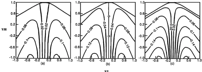
Figure

5 shows

contours

of &x for symmetric

transversely

isotropic

ridges

with horizontal

planes

of transverse

isotropy

where a - 1 and e - 0.1 (6.5% slope at inflection points). The ratios E/E' and G/G' vary between 1 and 4, v - 0.25, and v/v' varies between 1 and 3. These ratios cover the

ranges determined

experimentally

for a broad range of

anisotropic

rocks [Amadei

et al., 1987].

The overall

shape

of

the contours

of &x is influenced

by the elastic

constants

of

1.0 1 0.0- 0 -1.0 I

Y/H.

0'1-1.0

1.o -1.o o.o

1.o -1.o o.o (f)

Fig. 6. Contours of 6'x in the ridges with vertical planes of transverse isotropy parallel to the 9, • coordinate plane with a = 1, e = 0.1, and (a) E/E' = 1 and G/G' = 1, (b) E/E' = 1.5 and G/G' = 1, (c) E/E' = 4 and G/G' = 1, (d) E/E' = 1 and G/G' = 4, (e) E/E' = 1.5 and G/G' = 4, and (f) E/E' = 4 and G/G' = 4, with v = v' = 0.25.

1.0 1.0 1.0 0.6 0.2 -0.2 -0.6 -1.0 -1.0 -0.6 -0.2 0.2 0.6 1.0 -1.0 0.6 -0.2 0.2 0.6 1.0 -1.0 -0.6 -0.2 0.2 0.6

Y/•

(a)

(b)

(c)

-0.6

5•

Fig. 7. Effect of the ratios E/E' and G/G' on &z in the ridges with a = 1, e = 0.1, and (a) E/E' - 1 and G/G' 1, (b) E/E' = 1.5 and G/G' = 1, (c) E/E' = 4 and G/G' = 1, (d) E/E' = 1 and G/G' = 4, (e) E/E' = 1.5 and G/G' = 4, and (f) E/E' = 4 and G/G' = 4. Isotropy (Figure 7a) and horizontal anisotropy (Figures 7b-7f) with

3334 LiAO ET AL' GRAVITATIONAL STRESSES IN RIDGES AND VALLEYS 1.o •,- 1.0 1.0 0.6 0.6 0.6 -0.2 -0.2 -0.2

I

Fig. 8. Effect of the ratio E/E' on trxy in the ridges with a = 1, s = 0.1, and (a) E/E' -- 1 and G/G' = 1, (b) E/E'

= 1.5 and G/G' = 1, and (c) E/E' - 4 and G/G' - 1. Isotropy (Figure 8a) and horizontal anisotropy (Figures 8b and 8c) with v = v' = 0.25.

the transversely anisotropic rocks. As the ratio E/E' in- creases, the contours of &x follow the ridge shape, whereas the contours of &x deviate from the ridge shape as the ratios G/G' and •,/•,' increase. The magnitude of &x depends strongly on the rock's elastic properties. At a given point, &x increases with the ratio E/E'. On the other hand, as the ratio G/G' increases, &x decreases, especially around the axial plane (œ = 0). An increase in the ratio •,/•,' causes an increase in &x at the ridge crest but a decrease at greater depths.

Figure 6 shows the contours of &x in ridges exhibiting the vertical rock anisotropy shown in Figure 2c. For ridges consisting of comparable rock types, and at a given point, the magnitude of &x is the largest in the ridge exhibiting horizontal anisotropy and the smallest in the ridge with the planes of transverse isotropy that are vertical and parallel to the •, • coordinate plane.

Figure 7 shows contours of &z for a horizontally anisotro- pic symmetric ridge. The overall shape of the &z contours nearly follows the ridge shape. At a given point, &z increases with E/E' but slightly decreases as the ratio G/G' increases. The effect of •,/•,' on &z can be shown to be similar to the effect of •,1•,' on &x.

Contours

of tl'xy

for a horizontally

anisotropic

symmetric

ridge are shown in Figure 8. Zero shear stresses occur along the axial plane because of symmetry, and signs on both sides of the axial plane are different. As can be seen in Figure 8,

•'xy

increases

slightly

with the ratios

E/E'. Shear

stresses

can

also be shown to increase slightly with increases in •,/•,' but are not affected by any changes in G/G'.

Figure 9 shows contours of &x for symmetric orthotropic ridges where a = 1 and s = 0.1, exhibiting the anisotropy shown in Figure 2a. Different values of Young's modulus El, E2, E3 in the x, y, and z directions, respectively, are considered. The shear moduli G12 , G13 , and G23 are as- sumed to be equal and •q2 = •'2• - •'3• = •' = 0.25. Figure 9 shows that the variation of &x is affected by changes in Young's modulus E•, E2, and E' 3 and is dominated by the values of the Young's modulus (E2) in the vertical direction. As E 2 decreases and E1 increases, the value of &x greatly increases at a given point. The value of &x increases some- what as E1 increases with a decrease in E3. For orthotropic

ridges

it can be shown

that the trend in the variation

of •'xy

at

a given point (excluding points on the axial plane where

Y/It 1.0 1.0 1.0 0.0 0.0

' i.'

1

0 0.0

1.0

-1.0 -1.0

Fig. 9. Contours of &x for orthotropic ridges with a = 1, e = 0.1, and (a) E 1 = E, E2 - 1/3E, and E 3 = 1/2E' (b) E] = 1/3E, E2 = E, and E 3 = 1/2E; and (c) E 1 - 1/2E, E 2 -- E, and E 3 = 1/3E with G12 = G13 = G23 = G = E/2 (1 + v) and v]2 = v21 = v31 = v= 0.25.

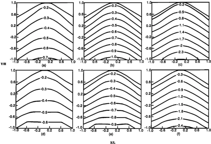
LIAO ET AL.' GRAVITATIONAL STRESSES IN RIDGES AND VALLEYS 3335 Y/l-i -0.5 -1.5 -2.5 -1.0 0.0 1.0 (a) -0.5 -1.5 -2.5 -0 5 5 5• 0.0 1.0 (b) -0.5 -1.5 -2.51 I . .. -1.0 3 (c) .0 0.0 1.0 -1.0 0.0 1.0 -1.0 0.0 (d) (e) (f)

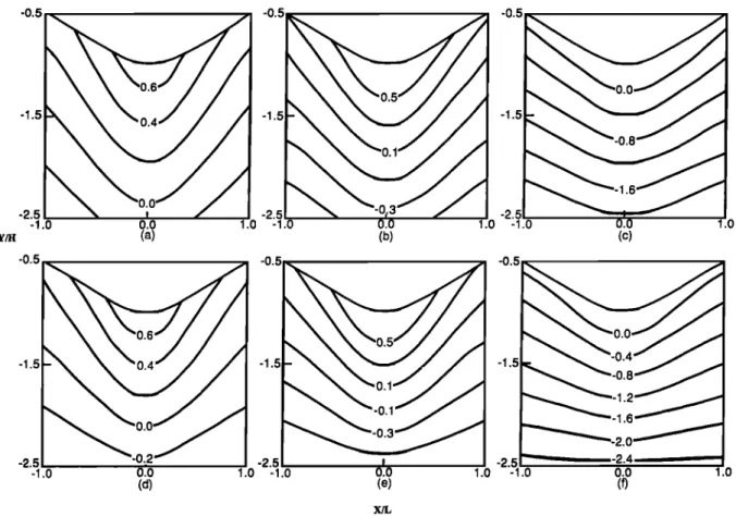
Fig. 10. Contours of &x for valleys with a = 2/3 and e = 0.1 for different rock types; (a) E/E' = 1 and G/G' = 1, (b) E/E' = 1.5 and G/G' = 1, (c) E/E' = 4 and G/G' = 1, (d) E/E' = 1 and G/G' - 4, (e) E/E' = 1.5 and G/G' = 4, and (f) E/E' = 4 and G/G' - 4. Isotropy (Figure 10a) and horizontal anisotropy (Figures 10b-10f) with v = v'

= 0.25.

1.0

1.0

there are no shear stresses) is similar to that for 6- x in the orthotropic case.

Figure 10 shows contours of &x in horizontally anisotropic symmetric valleys where a = 2/3 and s - 0.1 (9.75% slope at inflection points). This figure shows that a tensile region of

6-x develops

near the valley bottom in each case. The tensile

region decreases as E/E' increases and slightly decreases

with an increase of G/G'. It can be shown that as the valley broadens, the tensile zone increases for comparable rock

types.

The distributions of &x in orthotropic valleys with a = 1 and s = 0.1 (6.5% slope at inflection points) are shown in Figure 11. As expected, the gravitational stresses in the valleys are influenced by El, E2, and E 3. Figure 11 shows

-0.5 -0.5 -1.5 -1.0 1.0 -1.0 0.0 1.0 (a) (b) -0.5 -1.5

O

ø'ø

Fig. 11. Contours of &x for orthotropic valleys with a = 1, e = 0.1, and (a) E 1 = E, E 2 = 1/3 E, and E 3 -- 1/2 E; (b) E 1 = 1/3 E, E 2 = E, and E 3 = 1/2 E; and (c) E1 = 1/2 E, E 2 = E, and E3 = 1/3 E with G12 = G13 = G23 = G = E/2 (1 + v) and vl2 = v21 = v31 = v= 0.25.

3336 LIAO ET AL..' GRAVITATIONAL STRESSES IN RIDGES AND VALLEYS

that a tensile b- x develops in the valleys. The tensile region is

1 1

the largest

when

El = 7 E, E2 = E, and

E3 = • E and

is the

I 1

smallest

when

E• = •E, E 2 = E, and E3 = 7E'

Finally, as mentioned

previously,

by is independent

of the

elastic properties of the medium. Since the slopes are very

small,

the by stress

contours

follow the shape

of the ridge

or

valley, even near the surface.

CONCLUSIONS

The approximate solution presented here can be used to predict gravitational stresses in the near surface of laterally constrained isolated ridges or valleys with small slopes. This solution can be used for ridges or valleys consisting of isotropic, transversely isotropic, or orthotropic rocks. The magnitude of the predicted stresses is of the order of the characteristic stress p•7H, where p is the rock density, •7 is gravitational acceleration, and H is the characteristic height of the ridge or depth of the valley.

Horizontal gravitational stresses in anisotropic ridges with 6.5% slope depend strongly on the degree and orientation of rock anisotropy. Nonzero compressive stresses develop at or near the ridge crests for all ridges with differently consti- tuted rocks. For the transversely isotropic ridges shown, the

dimensionless

horizontal stresses, 6-

x and &z at a given

point, increase with the ratio E/E', that is, when the rock deformability in the vertical direction is larger than that in the horizonal direction. The stresses 6- x and b- z increase at the ridge crest and decrease at greater depth with an increase in v/v', but stresses are little influenced by changes in the

ratio G/G'. Dimensionless

shear

stresses

•xy are not affected

by the ratio G/G' but are slightly influenced by the ratios E/E' and v/v'. For the orthotropic ridges, Young's modulus

in the vertical direction is the most dominant factor for the

horizontal gravity-induced stresses. The horizontal gravity- induced stresses increase as the Young's modulus in the vertical direction decreases. Overall, at a given point in comparable ridges, gravitational stresses are the largest when the rock has horizontal transverse isotropy.

For the gravitational stresses in anisotropic valleys with 6.5% and 9.75% slopes, tensile regions of 6- x develop under the valleys. The extent of the tensile regions is influenced by the degree of anisotropy. For example, in the case of horizontal anisotropy, their extent decreases as the ratio E/E' increases, but the extent of the tensile regions is little influenced by a change in the ratio G/G'. Note also that gravitational stresses are influenced by changes in the valley slope. The tensile regions increase as the valley broadens.

It is important to note the limitations of the approximate solution presented here. This approximate solution, like solutions presented previously for isotropic ridges and val- leys, is limited to small slopes not exceeding 10%. For steeper slopes in anisotropic rock masses, numerical meth- ods are required.

Another limitation is that this solution applies, of course, only to symmetric ridges and valleys. Other topographic profiles will require the development of stress functions appropriate for those profiles. For some topographies, an approximate solution based on McTigue and Mei's [1981] Fourier transform method or numerical methods may be required.

Finally, the assumption of lateral constraint allows no

horizontal deformation. This condition, as McGarr [1988] emphasizes, is geologically unrealistic. However, the state of stress following from this assumption can be considered a reference state upon which tectonic stresses can be super- imposed [McTigue and Mei, 1981]. For example, a solution for the response in anisotropic media to far-field uniaxial tension and compression like that of McTigue and Mei [1981] could be derived by the methods given above and superim- posed on the reference state. Note that the hydrostatic reference state preferred by McGarr [1988] is obtained in the isotropic case when Poisson's ratio v is equal to one half.

REFERENCES

Amadei, B., Rock Anisotropy and the Theory of Stress Measure- ments, Springer-Verlag, New York, 1983.

Amadei, B., and W. Z. Savage, Gravitational stresses in regularly jointed rock masses, in Proceedings of the International Sympo- sium on Fundamentals of Rock Joints, edited by O. Stephansson, pp. 463-473, Centek, Lulea, Sweden, 1985.

Amadei, B., W. Z. Savage, and H. S. Swolfs, Gravitational stresses in anisotropic rock masses, Int. J. Rock Mech. Min. Sci. Geo- mech. Abstr., 24, 5-14, 1987.

Amadei, B., H. S. Swolfs, and W. Z. Savage, Gravity-induced stresses in stratified rock masses, Rock Mech. Rock Eng., 21, 1-20, t 988.

Gerrard, C. M., Background to mathematical modeling in geome- chanics: The roles of fabric and stress history, in Finite Elements in Geomechanics, edited by G. Gudehus, pp. 33-120, John Wiley, New York, 1975.

Jaeger, J. C., and N. G. W. Cook, Fundamentals of Rock Mechan- ics, 2nd ed., 369 pp., Chapman and Hall, London, 1976. Kreyszig, E., Advanced Engineering Mathematics, 5th ed., John

Wiley, New York, 1983.

Lekhnitskii, S. G., Some cases of the elastic equilibrium of a homogeneous cylinder with arbitrary anisotropy (in Russian), Prikl. Mat. Mekh., 2(3), 345-367, 1939.

Lekhnitskii, S. G., Theory of Elasticity of an Anisotropic Body, translated from revised 1977 Russian edition, Mir, Moscow, 1977. McGarr, A., On the state of lithospheric stress in the absence of applied tectonic forces, J. Geophys. Res., 93, 13,609-13,617,

1988.

McGarr, A., and N. C. Gay, State of stress in the Earth's crust, Annu. Rev. Earth Planet. Sci., 6, 405-436, 1978.

McTigue, D. F., and C. C. Mei, Gravity-induced stresses near topography of small slope, J. Geophys. Res., 86, 9268-9278, 1981. McTigue, D. F., and C. C. Mei, Gravity-induced stresses near axisymmetric topography of small slope, Int. J. Numer. Anal. Methods Geomech., 11,257-268, 1987.

Savage, W. Z., and H. S. Swo!fs, Tectonic and gravitational stresses in long symmetric ridges and valleys, J. Geophys. Res., 91, 3677-3685, 1986.

Savage, W. Z., H. S. Swolfs, and P.S. Powers, Gravitational

stresses in long symmetric ridges and valleys, Int. J. Rock Mech. Min. Sci. Geomech. Abstr., 22,291-302, 1985.

Ter-Martirosyan, Z. G., D. M. Akhpatelov, and R. G. Manvelyan, The stressed state of rock masses in a field body forces, Proc. Congr. Int. Soc. Rock Mech. 3rd, 2(part A), 569-574, 1974. Wei, Z. Q., and J. A. Hudson, Testing of anisotropic rock masses,

in Proceedings of the Conference on Applied Rock Engineering, pp. 251-262, University of Newcastle Upon Tyne, England, 1988. B. Amadei, University of Colorado, Department of Civil Engi- neering, Boulder, CO 80309-0428.

J. J. Liao, National Chiao Tung University, Department of Civil Engineering, tOOt Ta Hsuei Road, Hsinchu, Taiwan 30050.

W. Z. Savage, U.S. Geological Survey, Box 25046, MS 966, Denver Federal Center, Denver, CO 80225.

(Received June 24, 1991; revised November 6, 1991; accepted December 2, 1991.)