HALF-BAND FILTER DESIGN WITH ODD-POLYNOMIAL CHEBYSHEV-APPROXIMATION

(1)

Half-band filter design with odd-polynomial

Chebyshev approximation

W.-T. Chang M.-S. Lin

Indexing terms: Filters andfiltering, Design

Abstract: An efficient method for the design of the half-band filter is described. Both the characteristics of the time response and the frequency response of the half-band filter are fully utilised to reduce the computation time and to increase the computation accuracy. The algorithm is based on the Chebyshev approximation criterion and uses only odd-symmetry polynomials for frequency interpolation to meet the required frequency response of the half-band filter.

1 Introduction

The use of digital technique in signal processing has become very popular in many areas. In several applications, a system may even be required to handle data of different type with various sampling rates [ l ] . This raises the need for a rate conversion system. A tree structure composed of sections each capable of coping with a sampling rate change of two is currently the most widely used. The design of half-band filter for decimation and interpolation has received considerable attention in the past decade [&SI.

Mintzer [2] had shown that the half-band filter can be designed by the Parks and McClellan [12] procedure with symmetry constrain on the passband and the stop- band cutoff frequencies as well as with equal weighting on the passband and the stopband error. The filter thus designed is not optimum because of the quantisation error. Grenez [3] proposed a linear programming method with constrained Chebyshev approximation to design the half-band filter. The dense grid of points replacing the frequency axis is made symmetric with respect to 4 2 . The specifications of the half-band filter was exactly met with the Remez exchange algorithm [20]. The symmetry property of the extrema1 points is not fully utilised in the general Parks and McClellan procedure. The search for the new external points in the Remes algorithm is thus not optimised. Vaidyanathan and Nguyen [19] proposed another method which exploits knowledge about the coefficient of the impulse response of the half- band filter to reduce the design time.

An efficient design procedure based on the odd- polynomial interpolation technique for the half-band

Paper 8001G (ElO), fust received 30th August 1990 and in revised form 22nd February 1991

W.-T. Chang is with the Department of Communication Enginezring and Centre for Te1eunn"mnication Research, National Chiao Tung University, Hsinchu, Taiwan, Republic of China

M.-S. Lin is with the Computer and Communication Laboratory, Industry Technology Research Institute, Hsinchu, Taiwan, Republic of China

492

I

filter is presented. The frequency response is always guaranteed to be symmetric with respect to w = 4 2 . The computation time is about 3/8 of that of the P-M method in each iteration because of the use of only odd- coefficients. The resultant filter is guaranteed to be a half- band filter. A filter obtained using this procedure has the following properties:

(a) The even terms of the impulse response are zero (b) The searching time for the new external points can be reduced by one-half compared with the Parks- McClellan method

(c) The external points obtained will be symmetrical with respect to the quarter-Nyquist frequency

(d) The overall computation time can be reduced by at least 3/8 compared with that of the Parks-McClellan method and one quarter is found in the implementation.

2 Characteristics of half-band filter

Multirate digital signal processing concepts have recently become popular. The basic concept of multirate digital signal processing is that the sampling rate of signals to be processed in the same system can be different. The signal is decomposed in the frequency domain into different channels to reduce the bandwidth. The signal in each channel can be decimated to lower rates because of the reduction in bandwidth. The original signal can be reconstructed without error if these subsignals are properly recombined through interpolation.

If the factor of decimation and interpolation is two, a 2-band QMF bank will result. The system function of this filter bank is

X ( Z ) = %Ho(Z)Go(Z)

+

Hi(Z)Gi(ZII X ( Z )

+

fCHo(-Z)Go(Z)

+

Hi(-Z)Gi(Z)I

X ( - Z ) ( 1 )

The term containing X(-Z) is caused by the aliasing effect.

Smith and Barnwell [7, 81 proposed a method for the choice of the analysis and synthesis filters to reach the perfect reconstruction condition. The choices are

H , ( Z ) = Z-"-')H0(-Z-l)

G l ( Z ) = Z-"-"H1(Z-') (2) Go(Z) = Z-"-')Ho(Z-')

Using this, the transfer function can be written as T ( Z ) = F(Z)Z-"-"

+

F(-Z)Z-"-" (3) where F(Z) = Ho(Z)Ho(Z- '). For perfect reconstruction, the transfer function is required to be Z-"-'). From eqn. IEE PROCEEDINGS-G, Vol. 138, No. 4, AUGUST 1991

(2)

3, it is necessary that

F ( Z )

+

F ( - Z ) = 1 ₍₄₎

F(Z) is a linear phase FIR filter over the interval

[-(N

-

l), N - 13 and is called the half-band filter. From eqn. 4, it can be shown that the even terms off@) are zero except for f(0) = 0.5. If expressed in spectral domain (5) (6) F(w)

+

F(z

-

0) = 1 F ( 4 =

I

HO(4

IZ

and

From eqn. 5, it is clear that F ( 4 2 ) = 0.5. By this, eqn. 5

can be written as

(7) This means that F(w) is odd-symmetry with respect to

w = n/2. The design of this odd-symmetry filter is the main topic of this paper.

The P-M [12] algorithm is a popular method for linear phase FIR filter design. This method uses Cheby- shev approximation for frequency interpolation. It uses the Remes exchange algorithm to search external points during the iteration. The half-band filter is known to be an extra-ripple filter and is odd-symmetry with respect to

w = n/2, i.e. even terms must be zero. The P-M method can be used to design such a filter with equal weighting on both the pass band and the stop band and with symmetrical frequency response with respect to 4 2 . The even terms are not usually zero because of the quantisation error in the calculation. The filter obtained is not the half-band filter required. If the even term is deliberately set to zero to meet the requirement of the half-band filter, the resultant error ripple is not greater than that of the original [2]. This phenomenon indicates that a filter designed by the conventional P-M method is not optimal. The results from both the P-M method and the proposed odd-polynomial based method for the half- band filter design are to be compared.

The frequency response of the half-band filter is odd- symmetrical, so the search time for extreme points in the Remes exchange algorithm is reduced by half in the proposed method. The even terms of the time response are assumed to be exactly zero, so the size of the interpolation basis in the formulation is reduced by half. The proposed method is discussed in detail and the design formula is derived from the point of view of linear algebra.

3 Chebyshev approximation based on

An efficient technique to design the halfband filter with maximum stop band attenuation is presented. The filter spectral response is interpolated by a set of odd- polynomials. The Remes exchange algorithm is used to search the new extreme points in the Chebyshev approximation.

3.1 Chebyshev approximation

Chebyshev approximation [9] has long been used for optimisation designs such as network synthesis [lo]. The application of this in linear phase FIR filter design was proposed by Parks and McClellan [12]. Many tech- niques [ l l , 12, 17, 181 exist that can be used to solve this kind of optimisation problem. Linear programming and

odd-polynomial

IEE PROCEEDINGS-G, Vol. 138, No. 4, AUGUST 1991

the second Remes algorithm (the so-called Remes exchange algorithm) are the two most popular methods for solving the Chebyshev sensed optimisation problems.

The Remes exchange algorithm has fast convergence speed but is difficult to use or implement. Linear programming is easier and more flexible in use, but it is much slower in convergence than the Remes algorithm. The Remes exchange algorithm for optimisation in Cheby- shev approximation is discussed.

3.1 . I Problem modelling

Let {h(n)} be the impulse response of the product filter

over the interval [-(N - l), (N - l)]. The frequency response of the product filter can be described as

N - 1

H ( w ) = h(0)

+

2 4 ) cos (nw) 0

<

w

<

s (8) The Chebyshev approximation for the FIR filter design could be modelled as

" = l

(9) where W ( w ) is the weighting function of the approx- imation error, D(w) is the desired frequency response and A is a compact subset within CO, rr].

If the weighted error function of the approximation is written as

E(w) = W(O)[H(O) -

D(o)]

0 E A (10)

then the Chebyshev approximation can be rewritten in terms of E(w), as

3.1 2 Remes exchange algorithm

The basic concepts of Chebyshev approximation for filter design is as mentioned above. An iterative algorithm to solve this optimisation problem is discussed - the well known Remes exchange algorithm. This algorithm is simple and efficient, and is known [13, 141 to converge uniformly according to

I

- P*

I

< C$ and all com- ponents of the approximation must be continuous in A.

P

is the kth approximation polynomial, P* is the best approximation polynomial, C is a constant and o < e < i .

Several conditions and properties are first stated. Haar condition

Let {SI, gZ,

...,

gn} be a prescribed function set defined

on a compact metric space A. The system of functions {gi} is said to satisfy the Haar condition iff every gdx) is continuous in A for i = 1,

. . .

, n, and fer every set of n- vecrors {XI} with the form

X,

= [gl(xJ,

...,

g,,(xJ], i = 1,

.

. .

,

n, is linear independent for all distinct x, E A. That is, fgl, g 2 ,

.

. .

, gn} forms a basis of the n-space over A.

The linear combination

E,

c, g, is defined as the generalised polynomial. From the Haar condition, several properties can be obtained.

Property 3.1.1

If the set of functions {gl. g2, ..., g.} satisfy the Haar condition. There exists a square matrix M , such that

(3)

M(xl, x 2 ,

...,

x,) is clearly nonsingular, if the samples {xi}, i = 1,

. . .

,

n, are all distinct over A.

Property 3.1.2

Let { g l ,

...,

go} satisfy the Haar condition over A and span the n-space V", i.e., Vg in V", 3 ! { a f } , i = 1,

.

..,

n,

3 g =

xi

a i g f ) . If there is another function g n + l which is continuous on A. Thus {gl,

...,

gn, g n + l } would also satisfy the Haar condition if g n +

4

V".

Alternation theorem

Let { g l , g 2 ,

...,

g.} be a system of functions on A satisfying the Haar condition. For a given function f(x),

x E A, there is one generalised polynomial P =

If

c i g i that would be the best approximation off on A iff the error function r = f - P exhibits at least n

+

1 'alternations' on A. In other words, ifxi) = -r(xi+ 1) = k p , xo <

x ~ < . . . < x , , x E A

.

A means the interested regions of x and from this theorem, A must be chosen to have n

+

1 alternations or more, and p = max, E A

1

r(x)

1.

Iterative procedure

Let the functions

si}

satisfy the Haar condition, and Yx) = y(x)! f(x)

-ki

ci gi

I

is the weighted error function satisfying the alternation theorem on A. f(x) and W(x) are continuous on A. Let {xt,

$,

..

.,

x:} be the kth iteration extreme points, x t < x: <

. . .

< x:, x: E A, and

pk the deviation of the kth iteration according to the kth extreme points.

The solution of the Chebyshev approximation problems can then be obtained by the following iterative process:

(a) Initial guessing of the extreme points {xo}

(b) From alternation theorem, suppose in the kth iteration {x!} and pk satisfy

r 1

= ( - l ) ' p k i = O ,

...,

n (13)

j = 1 in matrix form

(14)

Assume g n + l ( x i ) = (- lY+'/W(xi), i = 0,

. . .

, n. If eqn. 14

is to be invertible, then from property 3.1.1 and 3.1.2, { g l ,

...,

g n , g n + l } has to satisfy the Haar condition. That is, g.+ is not in the n-space spanned by { g l ,

. . .

,g.}. If W(x) is chosen to satisfy the condition above, then the above system of equations can be solved to find pk and the kth approximation polynomial as

PL

=

I:=

c f gi(x)

(c) From the polynomial p.' to find new extreme points

{X!"}

(d) Check if {x;"} is exactly equal to {x!}, or equiva- lently, if pk+' is equal to pk. If not, go back to step b

(e) Pk is the best approximation polynomial to f ( x ) , and pk is the ultimate equal ripple deviation with respect to the weighting function W(x) on A. Denote this best approximation polynomial and deviation as P*(x) and

p*, respectively.

494

3 2 Polynomial interpolation [15, 161

The interpolation technique is one of the simplest ways to determine the original function in many applications. The spline curve is commonly used as the interpolation basis in curve-fitting applications. In many applications the problem is how to find a well defined interpolation basis that is suitable for the application. A method, based on the linear functional theory of linear algebra, is introduced to find the interpolation basis required for the application in question.

32.1 Linear functional theory [ 1 51

In the linear transformation domain, there exists a special case that transforms a n-dimensional vector space V" into a field F (i.e., one-dimensional vector space). If some specifications are given to the n-dimensional space basis of V", for example, let the basis be (1, x,

...,

x"-'}, this transformation that transforms from V" to F then acts like a linear function. A formal definition of this theory is presented in the following:

DeJinition

Let V" be a n-dimensional vector space over the field F ; 1 is a linear transformation from V" to F (denote I : V" -+

F)

and I satisfies

l ( c a + B ) = c l ( a ) + I ( / J ) V C E F and a , B E V " (15) Thus, I is defined as the linear functional on V".

Dual space

Let L(V", F ) V* represent the set of all the linear func- tionals from V" to F and {Il, I,,

...,

I,} be a set of linear functionals that satisfy

libi)

=

aij.

Here { g l , g 2 ,

. . .

,

g m } is the basis of V" and 6, = 6(i - j ) . It can be shown that {Il,

I , ,

.

. .

,

I.} is linearly independent and forms a basis of V*, that is, dim V* = dim V". V* is defined as the dual space of V" or linear functional space.

Theorem 3.2.1

Let V" be an n-dimensional vector space over F, B =

{ e l ,

g , , ..., g.} be an ordered basis for V", and B* = {Il, I,,

. .

.

, l"} be an ordered basis for V*. Then B* is the unique basis, such that

l i g j ) = hij i, j = 1, 2,

...,

n (16)

and B* is called the dual basis of B. For every g in V" and 1 in V*, g = a l g l + a , g ,

+

...

+ a , g , and 1 =

b,ll

+

b2 I,

+

. . .

+

b, I,. It can be easily shown that ai =

Ids)

bi = l(gi) i = 1,

. . .

, n (17)

Theorem 3.2.1 is an important property that will provide the theoretical foundation for finding the interpolation basis for some special applications.

32.2 Odd-polynomials

In many approximation applications, it is desirable to formulate the problems with a set of polynomial functions or a linear combination of some special functions, e.g., sine or cosine functions. For the present situation, if the complexity of analysis is considered, it is obvious that polynomial representation is the most suitable.

The desired filter spectral response has a symmetrical property. The ordinary technique, such as Lagrange interpolation, may not be able to take this characteristic into consideration, and will suffer from unnecessary com- putational complexity. The requirement for the half- IEE PROCEEDINGS-G, Vol. 138, No. 4, AUGUST 1991

(4)

band filter necessitates the even terms of its impulse response to be zero. This characteristic indicates that the spectral response consists of only odd power polynomials. There is no need to consider the polynomial of even power.

If this is included in the formulation,f(x) = a.

+

a,x

+

a, x2

+

.

. .

+ a," x'".

Since f(x) has odd-symmetry property, i.e., f(x) is an odd-function, then f ( x ) + f ( - x ) = O a n d

2(a0

+

a 2 x z + a 4 x 4

+

...

+

aznxZn) = O f(x) = a l x

+

a 3 x 3

+

...

+

a2n-1x2n-1 It is clear that aZi = 0, i = 0,

. .

.,

n, and

(18) By this, the function that satisfies eqn. 18 is defined as the odd-polynomial function. In the same way, the function that contains only even power terms, is called even- polynomial function.

32.3 Interpolation basis

The classical Lagrange interpolation formula is a general interpolation technique for arbitrarily spaced sample points. The Lagrange interpolation may be unsuitable in this case. A new interpolation formula that will satisfy the requirements must be designed.

Question modelling

Let B = {x, x3,

...,

x2"-'} be an ordered basis on V", and B' = {gl,

...,

gn} be another ordered basis on V" with

gi = bijX2'-1 (19)

j = 1

Let {f(xl),f(x2),

. . .

, f ( x , ) } be a set of n-distinct samples. Then, the question for finding an interpolation basis can be stated as follows :

A basis set B' = {gl,

. . .

, g"}, is desired that satisfies

n

f(x) =

,E

f ( x h 0 ) (20)

, = 1

It is known that the dual space basis B* =

{Il.

. . .

, la} and

U-)

= f ( X i ) (21)

Before solving this question, it is necessary to ensure that B* is indeed a basis of the dual space V*. This can be proved if {Il,

. . .

, lm} are linear independent.

Proof: Suppose {li}. i = 1,

. .

.

, n, are linearly dependent and {al,

...,

a,} are not all zero and ai E F, i = 1,

...,

n.

Such that

I = alll

+

a,l,

+

...

+

a,l, = 0 Then from theorem 3.2.1

l ( f ) =

,e

ai f(xi) = O V xi E F i = 1,

. . .

, n

It is clear that ai = 0, for i = 1,

. . .

, n and this contra- dicts the assumption. So {Il, I , ,

...,

I,} is linearly inde- pendent and forms a basis of V*.

"

, = 1

Solution of odd-polynomial basis

B* is a basis of the dual space, so from theorem 3.2.1 and eqn. 21

(22) gJ{xi) =

aij

i, j = 1, 2,

...,

n

IEE PROCEEDINGS-G, Vol. 138, N o . 4, A U G U S T 1991

Consider j = 1 and eqn. 19, eqn. 22 means that 1 i = l 0 otherwise bllxi

+

bl,x:

+

...

+

b l n x f " - ' = in matrix form A . B = C where and B = (bll b12

...

bJ C = ( l 0

...

0)'

It can be seen that A is similar to the Vandermone matrix and will be nonsingular, that is

det A = n x i

fl,

(x; - xf)

i = 1 l < i < J C # I

and will be nonzero for distinct {xi). So, eqn. 23 is invert- ible and

det A, det A

blk =

-

where A, is obtained by replacing the kth column of A

and C . From eqns. 19 and 25

gl(x) = det A,

.

x2'-'/det A k = l det A

Ix,

det A -- -

Similarly, for arbitrary j , say j = k, g, can be described as

x

n

(x2 - x ; , Xk

fi

(x: - x;) k = 1, 2,

...,

n (26) - j = l , j + k - j = l , j # k

This set of functions, {gl,

. . .

, gn}, is the interpolation basis required for the odd-polynomial function. The standard odd-polynomial interpolation formula can be expressed as

"

x

n

(x2

-4)

xi

n

(xf - x f ) f ( x ) = f(xJ j = y (27) i = 1 j = 1 . j # i Uniqueness theorem

Let B = {si} form an interpolation basis of V". If the two sample sets, { f(xJ} and {f'(xi)}, simultaneously satisfy

f(x) =

,E

f(xi)gAx) = f'(xi)gdx)

, = 1 , = 1

(5)

then

f(xJ =f'(xi) i = 1, 2, ..., n

Proof: Let f(x) = f(x,)gdx), if there exists another

set of samples

ET:,)}

which also satisfies f(x) =

Z=

1 f'(x,)gi(x). Then

0 =

c

(f(x3 -f'(x,)) ' gdx)

, = I

because {g,} is a basis of V", it is clear thatf(xi) =f'(xi), for i = 1,

.

. .

, n. Then it can be concluded that for any f(x) there exists a unique expression with {g,}.

3.2.4 Barycentric form

The interpolation method is very useful for recon- structing the original function from arbitrary spaced sample points. Unfortunately, it will take a lot of computations when the order of the interpolation is high. Hamming [I61 introduced a special barycentric form for Lagrange interpolation which has about n/2 fewer com- putations than that of the standard Lagrange interpolation formula. This form will make the interpolation technique more useful.

In the odd-polynomial case, if the desired functionf(x) is known for a given x, that is for a distinct sample set {x,}, i = 1,

.

.., n, thenf(x,) = xi.

From eqn. 27

because of the uniqueness property. If eqn. 27 is divided by eqn. 28 -

x:)l

'f(xk) f(x) = x

"='.

(29)

1

Cak/(x2 - ' xk t = 1 where

Eqn. 29 is the barycentric form for the odd-polynomial interpolation formula, and it has about (n

+

1)/3 fewer computations than that of the standard form.

3.3 Design method and procedure

There are many methods [Il, 12, 19,201 that can be used to design the half-band filter. Suppose { f ( n ) } , for n = -(N

-

l),

. .

.

, (N - 1) is the impulse response of the half-band filter and

N - 1

because F ( 2 )

+ F( -Z)

= 1, by applying eqn. 31

Clearly, eqn. 32 means that

0.5 n = 0 0.0 n = even

f

(4

=

{

4%

Sincef(0) is always a value of 0.5, it is more convenient to set f ( 0 ) to zero during the design process. The perfect reconstruction condition then becomes

F ' ( Z ) + F ' ( - Z ) = O and f'(2m)=O m 6 - Z (34) The dedgn for the half-band filter is to first design a linear phase filterf'(n) according to eqn. 34, and then let

f ( n ) =f'(n) andf(0) = 0.5.

3.3.1 Filter response represented in terms of

The condition for designing the perfect reconstructed half-band filter in eqn. 34 has been presented. Since the phase and f ( 0 ) are temporarily neglected, only the ampli- tude response is of concern

odd -polynomials

NI?. - 1

~ ' ( o ) = 2

1

f'(2n

+

1) cos (2n

+

1)w (35)

" = O

where N is even for the QMF design. It is clear that f ' ( N - 1) =f'( - N

+

1) = 0 if N is odd. So, only the case

when N is even is of concern.

Property 3.3

For a cosine function cos (no), if n = 2k

+

1, there is a set {a,}, i = 0,

.

.., k, such that

k

cos (2k

+

l)o = adcos w ) ~ , +

i = O

If n = 2k, then there is another set { b , } , i = 0,

. .

.,

k, such that

k

COS ( 2 k ) o = b&os w ) ~ ,

i = O

eqns. 36 and 37 can be combined as

cos (nu) = tni(cos o)i

i = O where i = 2 k + 1 n = 2 m + 1 t . =

"'

{

0 otherwise and bk i = 2 k 0 otherwise n = 2m t"i =

{

(37)

{t,,} i = 1,2,

.

..,

n, is the coefficient of the nth Chebyshev polynomial [9, 161 7',,(x) and eqn. 38 becomes

cos (no) = Tn(cos o) (39)

From property 3.3.1, eqn. 35 could be rewritten as

N / 2 - 1 F'(o) = 2

1

f"(n)(cos w)~"" (40) " = O where N/Z k = n f " ( n ) =

f'(2k

+

l )

.

t ( Z k + l ) ( Z n + l ) (41) and t(zk+l)(zn+l) is the (2n

+

1)th coefficient of the (2k

+

1)th Chebyshev polynomial. The half-band filter spectral response can be considered as an odd- polynomial function, and will be useful when applying the Remes exchange algorithm for finding the extreme points.

(6)

3 9 9 Iterative procedure

Since F'(w) = -F'(n - w), only the response during the interval CO, n/2] has to be considered. Let A denote the region [0, w p ] and up the passband edge. It has been shown that {cos (2i

+

l)o} and {(cos m)""}, i = 0, 1,

. . .

, N/2 - 1, satisfy the Haar condition in CO, 421. From the alternation theorem, there is a set of extreme points {mi}, m i E A , i = 0,

. . .

, N/2, and coo = 0 and mN12 = u p .

Since the half-band filter is an extra-ripple filter, the Chebyshev approximation for the half-band filter design then becomes

)

min

(

max W(m)

I

F'(w) - D ( o )

I

r o € I O . u J d

Apply the Remes iterative procedure as stated earlier, the following N/2

+

1 equations are obtained

det

( - V P

W ( 4 F ( q ) -

-

= D(mJ i = 0,

. . .

,

N/2 a1 a2 a" b , b ,

...

b , c I From eqn. 14 and

with respect to the two different bases. Here x i = cos mi. The weighting function W(w) is generally set to be unity because of band separability, and D(w) is set to be 0.5 so that the ultimate

1

F ( o )

1 <

p*, for w E [a,, n].

If eqn. 43 or 44 is solved directly and eqn. 35 or 40 is used to find the new set of extreme points, it will be time- consuming. In the following, a simple method, using the odd-polynomial interpolation basis discussed earlier, is presented and eqn. 27 can be restarted as

N / Z - 1 i = O

F(w) =

c

F(wi)gi+ 1(XJ

IEE PROCEEDINGS-G, Vol. 138, N o . 4, AUGUST 1991

(45)

where { g k } , k = 1 ,

...,

N/2, are the interpolation basis and satisfies eqn. 26. Thus eqn. 14 can be rewritten as

I

From eqn. 26

(47)

From eqns. 47 and 48, p and F'(wi) in eqn. 46 can easily be shown to be N / 2 k = O '(Ok) (50) p = N / 2

c

(- l ) ' a J W ( 4 k = O and

F(wi) = D(oJ

+

(- l)'p/W(~i)

i = 0, ..., N/2 - 1 (51) Since eqn. 46 is invertible and from eqn. 45

F ( w N / 2 ) = F ( m O ) g 1 ( X N / 2 )

+

'

.

'

+

F ' ( ~ N / z - l ) g N / 2 ( X N / 2 )

then, the condition

will be automatically satisfied. So, eqn. 51 is exactly the same as eqn. 42. Only the deviation p need be solved and F'(wi) will be obtained immediately.

It is more efficient to use the barycentric form in eqn. 29 than that of eqn.

44

and write F ( w ) as

F(aN/Z) = D ( w N / 2 )

+

(- 1 ) N ' 2 P / w ( m N / 2 ) N / 2 - 1

1

- xiI]F'(wt) F(w) = x k;;z- (52) - x : ) l x k k = 1 491

(7)

where

(53) ak = akx2

-

xi,,) k = 0,

. .

.

, N / 2 - 1

r - .

After several iterations, this procedure will converge, and the polynomial that best approximates the desired filter response will be obtained. The impulse response could then be calculated by taking the 2N points IDFT. This approximation is based on the odd-polynomial technique, so the best approximation P*(x) is guaranteed to be odd-symmetry with respect to w = x/2, and the inverse transformation would be

n = even (54)

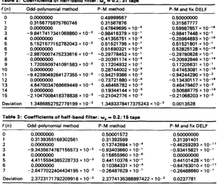
3.3.3 Normalisation

Since the definition of the half-band filter is F ( Z ) = H,(Z)H,(Z-'), the spectrum of F ( Z ) will be

I

H,(w)

1'.

It can be easily seen that F(w) must be non-negative for all

w. An adjustment is required to make F(w) greater than zero for w in [x/2, x ] . This can be achieved by adding the stop band deviation to the impulse response f ( 0 ) . If f ( 0 ) = 0.5 is to be maintained, a scaling to all the impulse

responses can be first applied and then a separate bias is added tof(0). The scaling factor and the bias factor were chosen to be (1

+

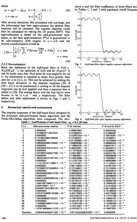
p)-' and p respectively. The filter before and after adjustment is shown in Figs. 1 and 2, respectively.

4 Numerical results and conclusions

The impulse responses of the half-band filters designed by the proposed odd-polynomial based algorithm and the Parks-McClellan algorithm were comnared. The devi-

ation p and the filter coefficients of three filters are listed in Tables 1, 2 and 3 with passband cutoff frequencies at

1

'"L

.o -0 . 2 -0 0.1 0.2 0.3 0.4 0.5 frequency, radians

Fig. 1 Halj-bundfilter before impulse response adjustment

'

0

l-ulQmu

0.1 0.2 0.3 0.L 0.5

frequency, radians

Fig. 2 Halj-bandfilter &er impulse response adjustment

"

Table 1 : Coefficients of half-band filter: up = 0.2; 63 taps

f ( n ) Odd-polynomial method P-M method P - M and fix DELF

0 0.5000000 1 0.31 688331 14447524 2 o.oooo00o 3 -0.1 01 89228831 68539 4 o.oo0ooO0 5 5.68660839661 00550 x 1 0-' 6 0.000oooo 7 -3.640349475373161 9 x lo-' 8 0.0000o0o 9 2.441 9601 528327786 x 1 O-' 10 0.000oooo 1 1 -1.6553439221 261 703 x

lo-'

12 0.000o0o0 13 1.1121337371768617 x

lo-'

14 0.o0ooO00 15 -7.3105661915249653 x 10.' 16 0.0000000 17 4.6535299490812190 x

lo-'

18 o.o0Oo0oo 19 -2.84031926656081 68 x lo-' 20 0.000oooo 21 1.6441 6972946771 1 1 x

lo-"

22 0,20815364 x 23 -8.9026472022364720 x 1 O-a 24 0.o0o0000 25 26 0.0000000 27 -1.9523598087233321 x 28 0.000o0oo 29 7.2256687490477233 x 30 0.0000000 31 Deviation 5.8635426463977397 x 1 0 - E 4.421 67409081 40399 x 1 0-4 -1.9781 40636441 1270 x 1 0-' 0.49997663 0.31 688333 0.22997244 x -0.1 01 89227 -0.21 782890 x 1 0-4 0.56866088 x

lo-'

0.1 9965335 x -0.36403461 x lo-' -0,17579249 x 0.24419587 x

lo-'

0.1 4952601 x

lo-'

0.50000000 0.31 688380 0.75975381 x 10.'' -0.10189371 -0.731 53564 x 1 0-14 0.56868309 x

lo-'

0.68201617 x -0.3640631 3 x

lo-'

-0.62368541 x 1 0-14 0.24422762 x

lo-'

0.55508948 x -0.1 6556697 x 10

'

-0.1 6553388 x

lo-'

-0.12161705 x

lo-'

-0.48492956 x 011121307~10-' 0.11124457 x lo-' 0.951 74840 x 10 - 0.41351402 x 10 ' 4 -0.73133593 x 10.' 0.46558763 x 10 0.29498009 x 10.'' -0.73104931 x 10.' -0.70589279 x -0.35042516 x 0.46534820 x 10-

'

0.501 57642 x -0.28402353 x 10.' -0.28421 697 x 10.' -033100121 x -0 25090159 x 0.16441241 x 10.' 0.2081 5364 x 1 O5 0.16455292 x

lo-'

0.21314520 x lo-'' -0.89019217 x 10.' -0.11609320 x -0.19186592 x 10.'' -0.89118005 x 10.' 0.44213563 x

lo-'

0.61545419 x 10.' 0.17472796 x 0.44273468 x 10.' -0.19518295 1 -0.19554197 x 10 -0.24318148 x 10.: 0.722501 65 x 10 0.72396340 10.' 0.10312851

lo.*

5.871 0522358252987 x 10.' 0.0000059 -0.16955132 x l o - " 0.16111451 x 10.'' -0.19752272 x 10.' -0.19827561 x 10.'

(8)

Table 2: Coefficients of half-band filter: W. = 0.2: 31 t a m

A‘

w,’ / I I I f ( n ) 0 1 2 3 4 5 6 7 8 9 10 1 1 12 13 14 15 Deviation Odd-polynomial method 0.000oooo 0.31 56775975760746 0.000oooo 0.0000000 5.1521577152782043 x

lo-’

-9.841 741 7341 069860 x 1 O-* 1.7205509741 091 583 x

lo-’

0.0000000 0.o0o0000 4.6470034769669449 x 10.’ o.o0oo0oo -2.1047008418378838 x

lo-”

1.34868527527791 99 x 1 0-3 -9.42390492641 27355 x P-M method 0.49999567 0.31 567876 0.47849695 x 1 0 - 5 -0.9841 6379 x

lo-‘

-0.41 355751 x 1 0 - 5 0.51 521 795 x

lo-’

0.51 690321 x 1 0 - 5 -0.29778452 x lo-‘ -0.20391 174 x 1 0 - 5 0.17204932 x lo-’ 0.28744002 x

lo-’

-0.94219386 x

lo-’

-0.73721880 x

lo-’

0.0000000 o.oooo00o -2.9870007475233616 x lo-‘ 0.46465782 x

lo-’

0,19344144 x 1.349337841 7375243 x -0.21042776 x

lo-*

P-M and fix DELF 0.50000000 0.31 567777 0.59987857 x

lo-‘’

-0.9841 7448 x

lo-’

-0.25964893 x

lo-’’

0.51521801 x

lo-’

0.52825128 x

lo-’”

-0.29780828 x lo-’ -0.20592846 x lo-‘’ 0.1 7205631 x

lo-’

0.47453081 x

lo-‘’

-0.94244290 x 1 0-’ -0.13430117

lo-’’

0.46479407 x

lo-’

0.50586775 x

lo-’’

-0.21068203 x

lo-’

0.001 3528

Table 3: Coefficients of half-band filter: W. = 0.2; 16 taps

f ( n ) Odd-polynomial method P-M method P-M and fix DELF

0.000oooo 0.50001 572 0.50000000 0.31 393551 69302561 0.31 392599 0.31 391401 0.000o0o0 0.0000000 0.1 5855960 x

lo-‘

0.0000oooo 4.41 15594365228733 x 1 0-’ o.oooo00o 0.1 3742684 x

lo-“

-0.93403660 x

lo-’

-0.46259293 x

lo-’’

-0.9341 5821 x

lo-’

-9.34356747871 55573 x 1 0-’ 0.441 10376 x lo-’ 0.44101428 x

lo-’

0.10384331 x -0.64763010 x lo-’’ -2.6477022404434195 x -0.26487629 x

lo-‘

-0.26488660 x lo-’ Deviation 2.37231 71792209918 x 10.’ 2 3774135388997422 x 10

’

0.0237781

0.18, 0.20 and 0.23, respectively. The deviation of the filter designed by the odd-polynomial based method is smaller than that of the P-M method. A better numerical accuracy is thus obtained. The third column of the Table is obtained by setting the DELF of the original Parks- McClellan program to 0.001. This made the dense grid of points replacing the frequency axis symmetric about n/2.

With this setting, the even terms of the filter coefficients by the P-M method were calculated to be zero to within the computer accuracy.

The barycentric interpolation formula of the odd- polynomial based method has 3/4 fewer multiplications than that of the P-M method. The odd-polynomial based method searches only one-half of the extreme points, so, in every iteration, there is a saving of 3/8 on the multipli- cations. That is, in every iteration, the odd-polynomial based method will be 3/8 times faster than the P-M method.

Another difference is the number of iterations required by the two methods. The P-M method uses only the N

+

1 extreme points for iteration. It needs an internal exchange among the N

+

2 extreme points. The odd-

Fig. 3

-A- odd-polynomial method . - A - - P-Mmethod

IEE PROCEEDINGS-G, Vol. 138, N o . 4. A U G U S T 1991 Computing time againstfilter length

uJp = 0.18

polynomial based method uses all the extreme points for iteration because of its symmetry property. It will thus require fewer iterations than the P-M method. For example, in Table 1, it takes only Seven iterations for the odd-polynomial based method and 12 iterations for the P-M method. A comparison between the computing time is shown in Figs. 3, 4 and 5, where an average gain of

’r

/A n 2

t

/‘ / /

,E

1

/ - 1 I I I IO 20 30 40 length Fig. 4 W I = 0.20

-A- odd-polynomial method - - A - - P-Mmethod

Computing time againstfilter length

/ / / / Fig. 5 w p = 0.23

-A- odd-polynomial melhod - - A - - P-Mmethod

Computing time againstfilter length

(9)

four for the proposed method over the P-M method is obtained.

5 Acknowledgment

The authors wish to thank the reviewers for their helpful comments. This work was supported by the National Science Council. under contract NSC-79-0404-E009-14.

6 References

1 CROCHIERE, R.E., and RABINER, L.R.: ‘Multirate digital signal processing’ (Prentice-Hall, Englewood c l i s , 1983).

2 MINTZER, F.: ‘On half-band, third-band and nth-band FIR filters and their design’, IEEE Tram., 1982, ASP-30, (S), pp. 734-738

3 GRENEZ, F.: Thebyshev design of filters for subband coders’,

IEEE Trans., 1988, ASP-36, pp. 182-185

4 VAIDYANATHAN, P.P.: ‘Quadrature mirror filter banks, M-band extensions and perfect reconstruction technique’, IEEE ASSP Mag., July 1987, pp. 4-20

5 VAIDYANATHAN, P.P.: Theory and design of M-channel maxi- mally decimated quadrature mirror filters with arbitrary M, having the uerfect reconstruction urovertv’. IEEE Trans.. 1987.

.

~

_ _

ASP-35. (4), pp. 476-492

6 VAIDYANATHAN, P.P., and HOANG, P.Q.: ‘The perfect- reconstruction O M F banks: new Architectures. solutions. and outi- ,~

mization strategies’, Proc. IEEE Int. Con$ Acoust., Speech, Signal

Processing, Dallas, April 1987, pp. 216!L2172

7 SMITH, M.J.T., and BARNWELL, T.P.: ‘A procedure for designing exact reconstruction filter banks for tree structure subband coders’,

IEEE ICASSP, San Diego, CA, March 1984, pp. 27.1.1-27.1.4 8 SMITH, M.J.T., and BARNWELL, T.P.: ‘Exact reconstruction

techniques for tree s t ~ c t u r e d subband coders’, IEEE Trans., 1986, 9 CHENEY. E.W.: ‘Introduction to auuroximation theory’ (Mffiraw-

ASP-34, (3), pp. 434441

_.

Hill, New York, 1966). Ch. 3

10 TEMES, G.C., and BINGHAM, J.A.C.: ‘Iterative Chebyshev approximation technique for network synthesis’, IEEE Trans., 1967, CT-14, pp. 31-37

11 RABINER, L.R., McCLELLAN, J.H., and PARKS, T.W.: ‘FIR didtal filter desien techniaues using weiahted Chebyshev auurox- ..

imhon’, Proc. IKEE, 1975,63, pp. 5 k 6 1 5

12 PARKS, T.W., and MrCLELLAN, J.H.: ‘Chebyshev approximation for non-recursive digital filters with linear phase’, IEEE Trans., 1972, CT-19, pp. 18%194

13 PARKS, T.W., and McCLELLAN, J.H.: ‘A program for the design linear Dhase finite h n u l s e resuonse filters’. IEEE Trans.. 1972 AU-24I,-pp 19S-199

‘FIR linear phase filter design program’, m ‘Programs for dietal signal urocessine’ (IEEE Press. 1979)

14 McCLELLAN, J H , PARKS, T W , and RABINER, L R

15 HUFFMIAN, K., and KUNZE, R.: ‘Linear algebra’ (Prentice-Hall, Englewood Cliffs, 1971)

16 HAMMING, R.W.: ‘Numerical methods for scientists and engi- neers’(Mffiraw-HiU, New York, 1962)

17 RABINER, L.R.: T h e design of finite impulse response digital filters using linear programming techniques’, Bell Syst. Tech. J., 1972, 51, (6), pp. 1177-1198

18 RABINER, L.R.: ‘Linear programming design of finite impulse response (F’IR) digital filters’, IEEE Trans., 1972, AU-U), pp. 28&288

19 VAIDYANATHAN, P.P., and NGUYEN, T.Q.: ‘A trick for the design of FIR half-band filters’, IEEE Trans., 1987, CAS34, (3). pp. 297-300

20 GRENEZ, F.: ‘Design of linear or minimum phase FIR filters by constrained Chebyshev approximation’, Signal Process, 1983, 5, pp. 325-332