Genetic Algorithm-Based Neural Fuzzy Decision
Tree for Mixed Scheduling in ATM Networks
Chin-Teng Lin, Senior Member, IEEE, I-Fang Chung, Her-Chang Pu, Tsern-Huei Lee, Senior Member, IEEE, and
Jyh-Yeong Chang, Member, IEEE
Abstract—Future broad-band integrated services networks based on the asynchronous transfer mode (ATM) technology are expected to support multiple types of multimedia information with diverse statistical characteristics and quality of service (QoS) requirements. To meet these requirements, efficient scheduling methods are important for traffic control in the ATM networks. Among the general scheduling schemes, the rate monotonic algorithm is simple enough to be used in high-speed networks, but it does not attain as high a system utilization as the deadline driven algorithm does. However, the deadline driven scheme is computationally complex and hard to implement in hardware. The mixed scheduling algorithm is the combination of the rate monotonic algorithm and the deadline driven algorithm; thus it can provide most of the benefits of these two algorithms. In this paper, we use the mixed scheduling algorithm to achieve high system utilization under the hardware constraint. Because there is no analytic method for the schedulability test of the mixed scheduling, we propose a genetic algorithm-based neural fuzzy decision tree (GANFDT) to realize it in a real-time environment. The GANFDT combines the GA and a neural fuzzy network into a binary classification tree. This approach also exploits the power of the classification tree. Simulation results show that the GANFDT provides an efficient way to carry out the mixed scheduling in the ATM networks.
Index Terms—Binary decision tree, deadline driven algorithm, quality of service (QoS), rate monotonic algorithm, recursive least square (RLS), schedulability test.
I. INTRODUCTION
T
HE broad-band integrated services digital networks (B-ISDN) is conceived to support a wide range of services such as video, voice, and numerical data. The asynchronous transfer mode (ATM) technique is considered the ground on which B-ISDN is to be built [4], [6]. ATM is a packet and connection-oriented switching technique and has the advantage of accommodating the variety traffic which possess different characteristics and service requirements. The diversity of traffic complicates the traffic control in the ATM networks, and thus the connection admission control (CAC) plays an important role among the traffic control functions. A new connection is accepted only when the network resources can provide enough bandwidth to ensure the required quality of service (QoS) while keeping high QoS.Manuscript received May 28, 2000; revised August 30, 2001 and December 27, 2001. This work was supported by the Ministry of Education under the Pro-gram for Promoting University Academic Excellence EX-91–E-FA06-4-4. This paper was recommended by Associate Editor A. Kandel.
The authors are with the Department of Electrical and Control Engineering, National Chiao-Tung University, Hsinchu 300, Taiwan, R.O.C.
Publisher Item Identifier S 1083-4419(02)03551-3.
Cell loss ratio and cell transfer delay are two important parameters to describe the QoS. Since the cell loss rate can be kept very low with the use of advanced transmission equip-ment, cell transfer delay is considered as the most important parameter in real-time communication services [20]. In order to meet diverse QoS, several packet multiplexing techniques have been proposed for different real-time applications [8], [9]. These schemes are different in traffic specification, system utilization, and implementation complexity. Among them, traffic-controlled rate-monotonic priority scheduling (TCRM) [9] provides bounded local delays to individual cells using a rate-monotonic priority scheduler. It is simple enough to be used in the high-speed ATM networks, but does not attain as high a system utilization as the deadline scheduling scheme, such as packet-by-packet generalized processor sharing (PGPS) [18], [19]. However, the deadline scheduling scheme is compu-tationally expensive because the priorities of connections need to be updated at every time slot.
In this paper, we use a mixed scheduling scheme to achieve high utilization under the hardware constraint in the ATM net-works. During the call set-up phase, when the schedulability test is successful for every switch along the path of the call, the new call can be accepted by the CAC. Because the condition for the schedulability test of the mixed scheduling involves a large set of inequalities and no analytic closed-form solution can be ob-tained, we propose a genetic algorithm-based neural fuzzy de-cision tree (GANFDT) to realize the mixed scheduling scheme efficiently. Neural networks and fuzzy systems have been ap-plied for ATM traffic control recently [2], [5], [22], because they are thought to have a lot potential in this area, especially for their learning and adaptive capabilities. The neural fuzzy net-works require no explicit model of the traffic, and the parallel structure of neural networks can be exploited in hardware im-plementations, which provides short response time. To obtain higher decision accuracy of the schedulability test, we combine the structure of the binary classification tree into our method. Bi-nary classification trees [1] and neural fuzzy networks are two popular approaches to the pattern recognition problems [3]. We use the GA-based neural fuzzy network at the decision nodes of a binary classification tree to extract linear and nonlinear traffic features. This scheme expands the capability of the clas-sification trees. Simulation results show that the system can at-tain high utilization by the mixed scheduling algorithm with the schedulability test performed by the proposed GANFDT.
The rest of this paper is organized as follows. Section II de-scribes the mixed scheduling algorithm of ATM cells. In Sec-tion III, we propose the GANFDT method to do the schedu-1083-4419/02$17.00 © 2002 IEEE
lability test for the mixed scheduling algorithm efficiently. In Section IV, we illustrate some simulation examples to justify the feasibility of our scheme. Concluding remarks are presented in Section V.
II. MIXEDSCHEDULING OFATM CELLS
The rate monotonic priority scheduling had been proved optimal among the fixed priority scheduling schemes [16] if a packet must be served before its succeeding packet of the same connection is generated. Packets can have variable length as in [16], but in this paper, we focus on fixed-length packets called
cells in ATM networks. The rate monotonic priority scheduling
scheme has the advantage of simple implementation. However, full processor utilization can be achieved by the deadline driven scheduling scheme with the cost of expensive implementation. In general, it needs a mechanism to update priorities and a sorting mechanism to select a packet for service.
The mixed scheduling is a combination of the rate monotonic scheduling and the deadline driven scheduling. We employ the mixed scheduling for transmitting cells to achieve high system utilization under the hardware constraint. If the mixed sched-uling scheme is not feasible at any switch along the path of the connection, the call request will be rejected by the CAC.
A. The Investigated System
Since ATM is a packet switching technique, it breaks the mes-sage up into cells of the same length (53 bytes). The basic com-ponents of an ATM network are ATM switches. Every switch has several input ports and several output ports. The main task for an ATM switch is transporting cells from its input ports to its destination output ports according to the predetermined routing table. To prevent excessive cell loss in the case of internal col-lisions of two or more cells competing for the same output port simultaneously, buffers should be provided within the switch.
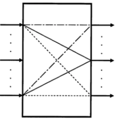
We can view the ATM switch as the combinations of eral multiplexers (see Fig. 1). A multiplexer multiplexes sev-eral signals originating from different customers onto a single access line. Cells which have the same destination output port are scheduled by a multiplexer. All incoming idle cells will be sorted out in an ATM multiplexer, thus concentrating the ATM traffic.
In this paper, we consider a multiplexer which accepts con-stant bit rate (CBR) traffic. That is, all connections generate cells periodically. We split time into time slots so that a slot is equal to the transmission time of a cell. We also normalize a slot to one unit time. Each connection is specified by its period which is assumed to be an integer. Let denote the period of connec-tion through this paper.
B. Three Scheduling Algorithms
A scheduling algorithm is a set of rules that determine which cell is to be served at a particular moment by a multiplexer. In this subsection, three priority driven scheduling algorithms are studied. First, a scheduling algorithm is said to be static if priorities are assigned to connections once and for all. A static algorithm is also called a fixed-priority scheduling algorithm. Second, a scheduling algorithm is said to be dynamic if priorities
Fig. 1. ATM switch.
of connections might change from cell to cell. Third, a sched-uling algorithm is said to be a mixed schedsched-uling algorithm if the priorities of some connections are fixed yet the priorities of the remaining connections vary from cell to cell.
For a particular priority assignment scheme, we say that a set of connections is schedulable if every cell is served before the arrival time of its succeeding cell. Rate monotonic scheduling algorithm is a fixed-priority scheduling algorithm which is op-timum in the sense that if a set of connections are schedulable by a fixed-priority assignment scheme, they must be schedulable by rate monotonic assignment scheme. Using the fixed-priority rate monotonic scheduling, connections with higher cell trans-mission rates (shorter periods) will have higher priority. That is, if , then connection has higher priority than connec-tion .
We define the utilization factor to be the fraction of processor time spent in the service of the cells. In other words, the uti-lization factor is equal to one minus the fraction of idle pro-cessor time. Since is the fraction of processor time spent in serving cells of connection , for a set of connections, the utilization factor is
Since the rate monotonic priority assignment is the optimum fixed priority assignment, the utilization factor achieved by the rate monotonic priority assignment for a given set of connec-tions is greater than or equal to the utilization factor of any other fixed priority assignment for the same set of connections. For a set of connections with fixed priority order, the least upper bound to processor utilization is [16], and for large , which approximates 70%.
On the other hand, the dynamic-priority deadline driven scheduling assigns the priorities to connections according to the deadlines of their current cells. That is, a connection will be assigned the highest priority if the deadline of its current cell is the nearest, and will be assigned the lowest priority if the deadline of its current cell is the furthest. In our case, the deadline of a current cell is the arrival time of the next cell for the same connection. Such a scheme of assigning priorities is a dynamic one, in contrast to a fixed priority scheduling in which priorities of connections do not change with time. Deadline driven scheduling policy is optimum in the sense that if a set
of connections can be scheduled by any algorithm, it can be scheduled by the deadline driven scheduling algorithm.
The employment of the mixed scheduling is motivated by combining the advantages of the above two scheduling poli-cies. The rate monotonic scheduling policy has the advantage of simplicity, while the deadline driven scheduling policy has the advantage of high system utilization. Specifically, if there are connections to be scheduled by the mixed scheduling al-gorithm, connections , the connections of shortest periods, will be scheduled according to the fixed-priority rate monotonic scheduling algorithm, and the remains, connections , be scheduled according to the deadline driven scheduling algorithm when the multiplexer is not occu-pied by connections . We use the mixed scheduling policy as the cell multiplexer for the efficiency of cell transmis-sion. Since one cell is permitted to be transmitted before the deadline, at most one cell will stay in the multiplexer at any time. Hence, the multiplexer needs a buffer of one cell for every connection.
C. Schedulability Test
To provide QoS guarantee with a scheduling scheme, schedu-lability test must be done at every involved switch. If the test fails at any switch along the path of a connection, the connec-tion request must be rejected. Here, the QoS guarantee means no cell should be lost and the delay of any connection cell at each switch is bounded by . Thus, when each cell arrives at the multiplexer with period , the multiplexer must finish trans-mission within time slots.
Since the deadline driven scheduling algorithm can achieve full utilization, its schedulability test condition is very simple. A set of connections are schedulable by the deadline driven sched-uling algorithm if and only if the system utilization factor is smaller than or equal to 1, i.e., .
The schedulability test of the rate monotonic scheduling al-gorithm for ATM networks has been discussed in [10]. Lee and Chang proved the following theorem in [10].
Theorem 1: A set of connections with periods is schedulable by the rate monotonic scheduling algorithm if and only if there exists an integer
such that and for all ,
.
The schedulability test at each switch with the mixed sched-uling scheme is similar to the one in [16]. Suppose there are CBR connections to be scheduled by the mixed scheduling
scheme. Assume that . Let
the cells of connections be scheduled according to the rate monotonic scheduling algorithm, and the cells of
con-nections be scheduled according to the
deadline driven algorithm when the multiplexer is not occupied by connections . The connections with shorter pe-riods are scheduled by the rate monotonic scheduling algorithm because if the connection with longer period has higher priority than the one with shorter period, it will impede the service of the connection with shorter period. In other words, if the connection with shorter period has higher priority than the one with longer period, more sets of connections have the opportunities to be
schedulable by the mixed scheduling. Thus, the system can have higher utilization. This can be seen with the following example. Let there be three connections with periods 2, 3, and 6, respec-tively. Clearly, the utilization factor is . When the connections with periods 2 and 3 are scheduled by the rate monotonic algorithm and the connection with period 6 is scheduled by the deadline driven algorithm, this set of connec-tions is schedulable. However, if the connecconnec-tions with periods 2 and 6 are scheduled by the rate monotonic algorithm and the connection with period 3 is scheduled by the deadline driven al-gorithm, this set of connections is not schedulable.
In addition, in Theorem 1, the integer represents a pe-riod, in which form a fixed schedulable pattern. In other words, every time slots, will be sent out in the same time sequence. The meaning of can be also caught from the proof of Theorem 1. Suppose is schedulable. Let be the slot packet that is served, where denotes the packet generated by connection . The number of connection ( ) packets served up to slot is and hence . Since is assumed to be schedu-lable, we have . Therefore, there exists an such that
and . Hence, is
schedulable implies the arguments in Theorem 1 must hold for
all , .
The schedulability test for the mixed scheduling involves an availability function . The availability function for a set of connections is defined as the accumulated transmission time slots from 0 to available to this set of connections. Let denote the availability function of the scheduler for connections
. Clearly, is a nondecreasing function of . Then, the schedulability test for the mixed scheduling with availability function is given by
(1)
for all s which are multiples of , or , or . From the above descriptions, we know that the schedulability test for the mixed scheduling police with availability function is given by (1) for all s which are multiples of , , , and . Hence, the above inequality should be checked for LCM time slots, where LCM is the least common multiple of
, , , and , which is equal to in the
worst case. The availability function in the above equation counts the sum of the empty time slots which are not occupied by connections until time . Hence, we have
To calculate , we need multiplications, additions, and supremum operations. Furthermore, we need multi-plications, additions, supremum operations, and one comparison operation in obtaining the left-hand side of (1). As a total, we need multiplications, additions, supremum operations, and one comparison operation in each inequality check in (1). Hence, the computation load of the
schedulability test of the mixed scheduling algorithm according to (1) is
multiplications additions supremums comparison
in the worst case. In short, this computation load can be written
as ( ) (operations).
Note that this condition is a necessary and sufficient condition. The left-hand side of (1) represents the sum of the needed service time slots which belong to connections between time 0 and time . The avail-ability function counts the sum of the empty time slots which are not occupied by connections until time . Conceptually, the schedulability condition implies that if the available empty time slots left by the rate monotonic connections are enough for the connections scheduled by the deadline driven scheduling policy, these connections are schedulable. This test involves the solution of a large set of inequalities and no analytic closed-form solution can be obtained, so its application is not easy to be dealt with in a real-time environment. In Section III, we shall propose a new scheme to do the schedulability test efficiently.
Lemma 1 that follows is induced from (1). It states that if a set of connections is schedulable by a mixed scheduling algorithm, it is also schedulable by the same algorithm except that a con-nection scheduled by the rate monotonic algorithm originally is changed to be scheduled by the deadline driven algorithm. This lemma will be used in Section IV-A.
Lemma 1: If a set of connections with periods is schedulable by the mixed scheduling algorithm with connections
scheduled by the rate monotonic algorithm, and connections scheduled by the deadline driven al-gorithm, then it is also schedulable by the mixed scheduling algorithm with connections scheduled by the rate monotonic algorithm, and connections
scheduled by the deadline driven algorithm.
Proof: At any moment, the total demand of service time
cannot exceed the total available service time. Thus, we must have
for any Since
we have
for any According to (1), this completes the proof.
III. GA-BASEDNEURALFUZZYDECISIONTREE In this section, we propose a GANFDT to do the schedu-lability test of the mixed scheduling algorithm. A classifica-tion/decision tree is a popular method for deciding boundaries of some classes. In our case, there are only a boundary be-tween schedulable class and unschedulable class to be found. We use a GA or a self-constructing neural fuzzy inference net-work (SONFIN) at each decision node of a classification tree to extract a feature. When the features represent the traffic charac-teristic better, the decision made by the tree can be more precise. To represent the traffic characteristic well, we choose the utiliza-tion factor and the connecutiliza-tion numbers of each traffic type as the input parameters of our GANFDT. Connections with the same period belong to the same traffic type. The single output of the GANFDT indicates whether the schedulability test is successful or not.
We shall introduce the GA and the SONFIN in Sections III-A and III-B, respectively. Then, the GA and SONFIN are com-bined with the binary classification tree to form the GANFDT method in Section III-C.
A. Basics of GA
The GA is a general purpose stochastic optimization method for search problems [11]. GAs differ from normal optimization and search procedures in several ways [12], [13]. First, the algo-rithm works with a population of strings, searching many peaks in parallel. By employing genetic operators, it exchanges in-formation between the peaks, hence lowering the possibility of ending at a local minimum and missing the global minimum. Second, it works with coding of the parameters, not the param-eters themselves. Third, the algorithm only needs to evaluate the objective function to guide its search, and there is no re-quirement for derivatives or other knowledge. The only avail-able feedback from the system is the value of the performance measure (fitness) of the current population. Finally, the tran-sition rules in GAs are probabilistic rather than deterministic. The randomized search is guided by the fitness values of each string and how they compare to others. Using the operators on the chromosomes which are taken from the population, the al-gorithm efficiently explores parts of the search space where the probability of finding improved performance is high.
The basic element processed by a GA is the string formed by concatenating substrings, each of which is a binary coding of a parameter of the search space. Thus, each string represents a point in the search space and hence a possible solution to the problem. Each string is decoded by an evaluator to obtain the objective function value of an individual point in the search space. This function value, which should be maximized or min-imized by the algorithm, is then converted to a fitness value which determines the probability of the individual undergoing genetic operators. The population then evolves from generation to generation through the application of the genetic operators. The total number of strings included in the population is kept unchanged through generations. A GA in its simplest form uses three operators: 1) reproduction; 2) crossover; and 3) mutation. An abstract procedure of a simple GA is shown in Fig. 2.
Fig. 2. Basic steps of GA.
B. Self-Constructing Neural Fuzzy Inference Network (SONFIN)
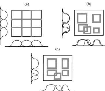
The SONFIN is a fuzzy rule-based network possessing learning ability. Compared with other existing neural fuzzy networks [7], [21], [23], a major characteristic of the network is that no preassignment and design of the rules are required. The rules are constructed automatically during the on-line operation. Two learning phases, the structure as well as the pa-rameter learning phases are adopted on-line for the construction task. One important task in the structure identification of the SONFIN is the partition of the input space, which influences the number of fuzzy rules generated. Traditional partitioned results are shown in Fig. 3(a) and (b) [13]. Fig. 3(a) is a grid-type partitioned result [7], [23]. A major problem of this kind of partitioning is that the number of fuzzy rules increases exponentially as the dimension of the input space increases. Fig. 3(b) is a clustering-based partitioned result [15], [17], [23]. Compared with the grid-type partition, the number of rules is reduced by this method, but not the number of membership functions in each dimension. In fact, by observing the projected membership functions in Fig. 3(b), we can find that some mem-bership functions projected from different clusters have high overlapping degrees. These highly overlapping membership functions can be eliminated. An on-line input space partitioning method, the aligned clustering-based method, is proposed in this paper. The on-line partitioned result is shown in Fig. 3(c).
This method will reduce not only the number of rules gener-ated, but also the number of fuzzy sets in each dimension. An-other feature of the SONFIN is that it can optimally determine the consequent part of fuzzy IF–THEN rules during the structure learning phase. A fuzzy rule of the following form is adopted in our system initially
Rule IF is and and is
THEN is (2)
Fig. 3. Fuzzy partitions of a two-dimensional (2-D) input space. (a) Grid-type partitioning. (b) Clustering-based partitioning. (c) Proposed aligned clustering-based partitioning.
where
and input and output variables, respectively; fuzzy set;
position of a symmetric membership function of the output variable with its width neglected during the defuzzification process.
Then, by monitoring the change of the network output error, ad-ditional terms (the linear terms used in the consequent part of the TSK model [21]) will be included when necessary to further reduce the output error. This consequent identification process is employed in conjunction with the precondition identification process to reduce both the number of rules and the number of consequent terms. For the parameter identification scheme, the
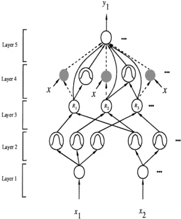
Fig. 4. Structure of the SONFIN.
consequent parameters are tuned by the recursive least square (RLS) algorithm, and the precondition parameters are tuned by the back-propagation (BP) learning algorithm. Both the struc-ture and parameter learning are done simultaneously to achieve fast learning.
In this subsection, the structure of the SONFIN as shown in Fig. 4 is introduced. With this five-layered network structure of the SONFIN, we shall define the function of each node for the SONFIN in Section III-B1, and the learning algorithm of the SONFIN in Section III-B2.
1) Structure of the SONFIN: Let and denote the input and output of a node in Layer , respectively. The func-tions of the nodes in each of the five layers of the SONFIN are described as follows.
Layer 1: No computation is done in this layer. Each node in
this layer, which corresponds to one input variable, only trans-mits input values to the next layer directly. That is
(3)
Layer 2: Each node in this layer corresponds to one linguistic
label (small, large, etc.) of one of the input variables in Layer 1. In other words, the membership value which specifies the degree to which an input value belongs a fuzzy set is calculated in Layer 2. With the use of Gaussian membership function, the operations performed in this layer is
(4)
where and are, respectively, the center (or mean) and the width (or variance) of the Gaussian membership function of the th term of the th input variable . Unlike other clustering-based partitioning methods, where each input variable has the same number of fuzzy sets, the number of fuzzy sets of each input variable is not necessarily identical in the SONFIN.
Layer 3: A node in this layer represents one fuzzy logic rule
and performs precondition matching of a rule. Here, we use the following AND operation for each Layer-3 node
(5) where is the number of Layer 2 nodes participating in the IF part of the rule.
Layer 4: This layer is called the consequent layer. Two types
of nodes are used in this layer, and they are denoted as blank and shaded circles in Fig. 4, respectively. The node denoted by a blank circle (blank node) is the essential node representing a fuzzy set (described by a Gaussian membership function) of the output variable. Only the center of each Gaussian membership function is delivered to the next layer for the local mean of max-imum (LMOM) defuzzification operation [14], and the width is used for output clustering only. Different nodes in Layer 3 may be connected to a same blank node in Layer 4, which means that the same consequent fuzzy set is specified for different rules. The function of the blank node is
(6) where , the center of a Gaussian membership func-tion. As for the shaded node, it is generated only when neces-sary. Each node in Layer 3 has its own corresponding shaded node in Layer 4. One of the inputs to a shaded node is the output delivered from Layer 3, and the other possible inputs (terms) are the input variables from Layer 1. The shaded node function is
(7) where the summation is over all the inputs and is the cor-responding parameter. Combining these two types of nodes in Layer 5, we obtain the whole function performed by this layer for each rule as
(8)
Layer 5: Each node in this layer corresponds to one output
variable. The node integrates all the actions recommended by Layers 3 and 4 and acts as a defuzzifier with
(9)
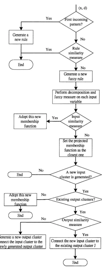
2) Learning Algorithm for the SONFIN: In Fig. 5, we use a
flowchart to illustrate the entire learning process of SONFIN. Here, two types of learning, namely, structure and parameter learning, are used concurrently for constructing the SONFIN. The structure learning includes both the precondition and con-sequent structure identification of a fuzzy IF–THEN rule. There are no rules (i.e., no nodes in the network except the input/output
Fig. 5. Flowchart for the learning process of SONFIN.
(I/O) nodes) in the SONFIN initially. They are created dynam-ically as learning proceeds upon receiving on-line incoming training data by performing the following learning processes si-multaneously: a) I/O space partitioning; b) construction of fuzzy rules; c) consequent structure identification; and d) parameter identification. Processes a), b), and c) belong to the structure learning phase and process d) belongs to the parameter learning
phase. The details of these learning processes are described in the rest of this subsection.
a) Input/output space partitioning: The way the input
space is partitioned determines the number of rules extracted from training data as well as the number of fuzzy sets on the universal of discourse of each input variable. For each incoming pattern , the strength a rule is fired can be interpreted as the degree the incoming pattern belongs to the corresponding cluster. For computational efficiency, we can use the firing strength given in (5) directly as this degree measure
(10)
where , , and
. Using this measure, we can ob-tain the following criterion for the generation of a new fuzzy rule. Let be the newly incoming pattern. Find
(11) where is the number of existing rules at time . If
, then a new rule is generated, where is a prespecified threshold that decays during the learning process. Once a new rule is generated, the initial centers and widths are set as
(12) (13) according to the first-nearest-neighbor heuristic [14], where
decides the overlap degree between two clusters. After a rule is generated, the next step is to decompose the multidimensional membership function formed in (12) and (13) to the corresponding one-dimensional (1-D) membership tion for each input variable. For the Gaussian membership func-tion used in the SONFIN, the task can be easily performed as
(14) where and are, respectively, the projected center and width of the membership function in each input dimension. To reduce the number of fuzzy sets of each input variable and to avoid the existence of redundant ones, we should check the sim-ilarities between the newly projected membership function and the existing ones in each input dimension. Since bell-shaped membership functions are used in the SONFIN, we use the for-mula of the similarity measure, , of two fuzzy sets
and with membership function
and , respectively.
Assume , we can compute by
where . Therefore, the approximate simi-larity measure is
(16)
where we use the fact that . Let
represent the Gaussian membership function with center and width . The whole algorithm for the generation of new fuzzy rules as well as fuzzy sets in each input dimension is as follows. Suppose no rules are existent initially.
IF is the first incoming pattern THEN do
PART 1. Generate a new rule,
with center , width ,
where is a prespecified constant.
After decomposition, we have 1–D membership functions,
with and ,
.
ELSE for each newly incoming , do
PART 2. find ,
IF
do nothing ELSE
,
generate a new fuzzy rule, with ,
.
After decomposition, we have
, ,
.
Do the following fuzzy measure for each input variable :
, ,
where is the number of parti-tions of the th input variable.
IF ,
THEN adopt this new membership function, and set ,
ELSE set the projected member-ship function as the closest one.
In the above algorithm, the threshold determines the number of rules generated. For a higher value of , more rules are generated, and in general, a higher accuracy is achieved. determines the number of output clusters gen-erated and a higher value of will result in a higher number of output clusters. is a scalar similarity criterion which is monotonically decreasing such that higher similarity between two fuzzy sets is allowed in the initial stage of learning. For
the output space partitioning, the same measure in (11) is used. Since the criterion for the generation of a new output cluster is related to the construction of a rule, we shall describe it together with the rule construction process in learning process b) below.
b) Construction of fuzzy rules: As mentioned in learning
process a), the generation of a new input cluster corresponds to the generation of a new fuzzy rule, with its precondition part constructed by the learning algorithm in process a). At the same time, we have to decide the consequent part of the generated rule. Suppose a new input cluster is formed after the presenta-tion of the current input–output training pair ( , ), then the consequent part is constructed by the following algorithm.
IF there are no output clusters,
do PART 1 in Process a), with re-placed by
ELSE do
find .
IF
connect input cluster to the existing output cluster ,
ELSE
generate a new output cluster,
do the decomposition process in PART 2 of Process a),
connect input cluster to the newly generated output cluster.
.
The algorithm is based on the fact that the preconditions of different rules may be mapped to the same consequent fuzzy set. Compared to the general fuzzy rule-based models with singleton output, where each rule has its own individual singleton value [17], [23], fewer parameters are needed in the consequent part of the SONFIN, especially for the case with a large number of rules.
c) Consequent structure identification: Until now, the
SONFIN contains fuzzy rules in the form of (2). Even though such a basic SONFIN can be used directly for system mod-eling, a large number of rules are necessary for modeling sophisticated systems under a tolerable modeling accuracy. To cope with this problem, we adopt the spirit of the TSK model [21] into the SONFIN. In the TSK model, each consequent part is represented by a linear equation of the input variables. It is reported in [21] that the TSK model can model a sophisticated system using a few rules. Even so, if the number of input and output variables is large, the consequent parts used in the output are quite considerable, some of which may be superfluous. To cope with the dilemma between the number of rules and the number of consequent terms, instead of using the linear equation of all the input variables (terms) in each rule, we add these additional terms only to some rules when necessary. The idea is based on the fact that for different input clusters, the corresponding output mapping may be simple or complex.
For simple mapping, a rule with a singleton output is enough. While for complex mapping, a rule with a linear equation in the consequent part is needed. The criterion for deciding which type of consequent part should be used for each rule is based on computing
(17)
where
firing strength of rule ; number of rules; desired output; current output;
accumulated error caused by rule .
By monitoring the error curve, if the error does not diminish over a period of time and the error is still too large, we shall add linear combinations of input variables to the rules, the values of which are larger than a predefined threshold value.
d) Parameter identification: The parameter identification
process is done concurrently with the structure identification process. The idea of BP is used for this supervised learning. Considering the single-output case for clarity, our goal is to min-imize the error function
(18)
where is the desired output, and is the current output. The parameters in Layer 4 are tuned by the RLS algorithm as
(19) (20)
where
forgetting factor; current input vector;
corresponding parameter vector; covariance matrix.
The initial parameter vector is determined in the structure learning phase and , where is a large positive constant. As to the free parameters and of the input membership functions in Layer 2, they are updated by the BP algorithm. Hence, by using the chain rule, we derive the error transmission in Layer 3 and the update of the parameters and in Layer 2 in the following.
Layer 3: Only the error signal needs to be computed in this
layer (21) where (22) if if . (23)
Layer 2: Using (4), the update rule of is derived as in the following:
(24)
where
(25)
if term node is connected to rule node otherwise.
(26) Therefore, the update rule of is
(27)
Similarly, using (4), the update rule of is derived as
(28)
where
if term node is connected to rule node otherwise.
(29) Therefore, the update rule of is
(30)
C. GA-Based Neural Fuzzy Decision Tree (GANFDT)
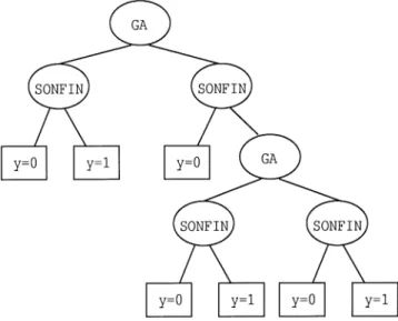
In this subsection, we combine the GA and SONFIN men-tioned in Sections III-A and III-B with the binary classification tree structure to form the GANFDT. A classification tree is a popular form of decision rules. A binary classification tree is
Fig. 6. Binary classification tree for a 2-class problem.
shown in Fig. 6 [3]. The circular nodes are decision nodes and square nodes are terminal nodes. Each decision node has a func-tion and a number associated with it. The tree classifies an input pattern vector through a chain of binary decisions. Starting at the root node and proceeding down the tree, tests of the form are conducted to determine whether the pat-tern goes to the left or right descendant. Each such test is called a splitting rule, and and are the associated feature and threshold, respectively. The pattern is assigned the class label of the terminal node it lands. In Fig. 6, indicates the un-schedulable class; indicates the schedulable class.
The power of the classification tree lies in the fact that ap-propriate features can be selected at different nodes and levels in the tree. In many pattern recognition problems, classifica-tion trees use coordinate features or linear features. However, difficult problems with complex decision boundaries may re-quire nonlinear features. Such features would further simplify the splitting procedure, and hence decrease the error rates and tree size. In this paper, we propose a method for extracting cer-tain coordinates and nonlinear features at the decision nodes of a classification tree. This method employs a GA or a SONFIN at each decision node to extract a feature. The idea of using the GA in the decision tree is to partition the training data into two suitable groups, which make the learning of the SONFIN easier. Furthermore, by adjusting the fitness function of the GA, we can get the desired learning result.
Our GANFDT method is designed to perform the schedula-bility test of the mixed scheduling algorithm. Thus, the input vector of the SONFIN must contain the parameters which rep-resent the traffic characteristic sufficiently, and the single output indicates whether or not the test is successful. We select the utilization factor and the number of connections for each type of traffic as the input parameters. Connections with the same pe-riod belong to the same traffic type. The desired output of the SONFIN is equal to one if the test is successful; otherwise, it is equal to zero.
During the tree growing phase, a tree is grown by recursively finding splitting rules until all terminal nodes have almost pure class membership or cannot be split anymore. The feature at a node is determined by optimizing a splitting criterion. In our decision tree, nodes at the odd layers use the GA to find the threshold for , so that nodes at the even layers can use the SONFIN to learn the decision boundary easily (see Fig. 7). At a node of the odd layers, if the utilization factor of an input vector is less than , this input vector is split to the
Fig. 7. Proposed binary classification tree with a GA or a SONFIN to extract a feature at each decision node.
left child of the original node; otherwise, it is split to the right child of the node. After that, the members of the left child and the members of the right child are trained by two SONFINs, re-spectively. The fitness function of the GA is basically the clas-sification rate of these two SONFINs. In a real situation, we prefer not to mistake an unschedulable set of connections for a schedulable one, so we consider that the classification rate of the unschedulable ones are more important than that of the schedulable ones. This can be achieved by amending the fitness function properly. The above process will be repeated until each terminal node contains almost the same class patterns and the classification rate cannot be improved anymore.
IV. SIMULATIONS
In this section, we illustrate some simulation examples to jus-tify the feasibility of the proposed GANFDT method.
A. Problem Formulation
Assume that there are four types of traffic scheduled by the mixed scheduling algorithm with periods and ,
respectively, where . Let ,
represent the number of connections with period . Let represent the periods of
connec-tions, where and if and only if
. Define if
. In other words, s are arranged in order so that
, and for
each . Thus, the utilization factor is . In our simulations, s are randomly generated between 1 and for a set of connections under the restriction that must be smaller than or equal to 1, because it is clear that when the utilization factor is larger than 1, the set of connections cannot be sched-uled by any algorithm. Let denote the largest number of connections which hardware can handle by the deadline driven algorithm. This constraint exists in the real-time environment because the computation and sorting time of the deadlines of the cells at every time slot is very considerable. Therefore, at
TABLE I
COMPARISON OFTWOMIXEDSCHEDULINGPOLICIES
most, connections can be scheduled by the deadline driven algorithm in the mixed scheduling policy; others are scheduled by the rate monotonic algorithm.
Some experiments are simulated, and about 6000 sets of connections are generated for each experiment. Since the least upper bound of the utilization factor is for the rate monotonic scheduling algorithm [16], a set of connections with utilization factor under 0.693 must be schedulable by the mixed scheduling algorithm. This can be proven by letting in Lemma 1. Hence, when we collect the 6000 patterns for each experiment, we only choose the patterns the utilization factors of which are larger than 0.693 and smaller than 1. The desired output for each input pattern is attained by checking (1) for LCM times, where LCM is the least common multiple of periods and . We check (1) for LCM times because the same situation is repeated for every LCM time slots. Among the 6000 patterns, we find that all the unschedulable ones have the utilization factors larger than some threshold, and this threshold is much larger than 0.693. We denote this threshold by , and only the patterns which have the utilization factor larger than are selected to train the GANFDT.
Before we do the schedulability test by using the GANFDT, we test the sets of connections which are scheduled by the rate monotonic algorithm with Theorem 1, so that we can ensure the connections scheduled by the rate monotonic algorithm will not be misclassified. As for the connections scheduled by the deadline driven algorithm, although the classification rate of the GANFDT can be very high after the training process, we still cannot ensure it will not misjudge any possible set of connec-tions. This problem must be solved because an unschedulable connection which is misclassified to be schedulable will cause data loss. Therefore, we provide another service which allows the renegotiation of a connection that is scheduled by the dead-line driven algorithm when data loss occurs. Such connections will be charged lower than other connections and are allowed to be scheduled by either deadline driven or rate monotonic al-gorithms decided by our system, and other connections are all scheduled by the rate monotonic algorithm. This kind of service is only for type-4 traffic with period , because if other traffic with a shorter period is scheduled by the deadline driven algo-rithm and some traffic with period is scheduled by the rate monotonic algorithm, the system utilization will decrease dras-tically. In other words, if the connection with longer period has higher priority than the one with shorter period, it will impede the service of the connection with shorter period and may make this set of connections unschedulable. This phenomenon can be seen in Table I. We generate 6000 sets of connections consisting of four types of traffic randomly and show the experiment results in Table I. In the first experiment, we randomly divide the type-4 connections into two groups: one for rate monotonic scheduling
TABLE II
(a) PERFORMANCECOMPARISON OF THESONFINANDBP NETWORKUNDER THESAMEMSE (CASE1). (b) PERFORMANCECOMPARISON OF THESONFIN
ANDBP NETWORKWITH THESAMELEARNINGTIME. (c) PERFORMANCE
COMPARISON OF THESONFINANDBP NETWORKUNDER THESAMEMSE (CASE2). (d) PERFORMANCECOMPARISON OF THEGANFDTANDBP NETWORKUNDER THESAMEMSE. (e) PERFORMANCECOMPARISON OF
THEGANFDTANDBP NETWORKWITH THESAMELEARNINGTIME. THEPERCENTAGEINDICATES THEPERCENT OFPATTERNSTHATARE
MISCLASSIFIED. NOTETHAT THERESULTS OFTABLES(a)AND(c) CAME
FROMDIFFERENTSETTING OFLEARNINGPARAMETERS INSONFIN
TABLE III
PERFORMANCECOMPARISON OFFOURDIFFERENT
SONFIN-BASEDCLASSIFIERS
and the other for deadline driven schedulin. All the other types of connections are scheduled by the rate monotonic scheme. In the second experiment, we randomly divide each type of con-nections into two groups, one for rate monotonic scheduling and the other for deadline driven scheduling. The parameters are set
as , , , , and .
If more than connections are to be scheduled by the deadline driven algorithm, we shall let the excessive connections with shorter periods be scheduled by the rate monotonic algorithm. It shows that when all types of connections are allowed to be scheduled by the deadline driven algorithm, the system utiliza-tion decreases significantly.
So far, we can summarize that there are six inputs to the
SONFIN; they are denoted by , and ,
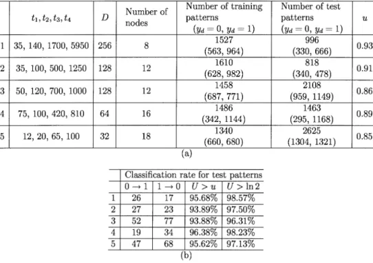
TABLE IV
(a) PARAMETERSUSED IN THEFIVEEXPERIMENTS FOR THEGANFDT. (b) CLASSIFICATIONRESULTS OF THEFIVEEXPERIMENTS BYUSING THEGANFDT
scheduled by the rate monotonic algorithm and by the deadline driven algorithm, respectively, and .
In the simulations, the fitness function of the GA is defined by
where is the number of the correctly classified unschedu-lable sets of connections and is the number of the correctly classified schedulable sets of connections. Since we prefer not to mistake an unschedulable set of connections for a schedulable one, is considered more important than and is multiplied by a scalar in the fitness function. In the GA, the parameter is coded by 8 b, the population size is 20, and the crossover and mutation probabilities are 0.8 and 0.01, respectively, where a single-bit mutation is used. After 20 generations, the process stops and the one with the highest fitness value is chosen. If the numbers of the unschedulable and schedulable sets of connec-tions are, respectively, and at a node of the decision tree, where , the tree growing phase will stop when is smaller than 20. This is based on our experiences that when
is smaller than 20, the class is pure enough and the clas-sification rate is hard to be improved any more by the GANFDT.
B. Simulation Results
In Table II, we compare the performance of two neural net-works: 1) the BP network and 2) SONFIN, to illustrate why we use the SONFIN in this paper. The BP network is the most pop-ular neural network, and the details of the BP network can be found in [14]. The symbol “ ” in Tables II and III repre-sents the number of unschedulable sets of connections that are misclassified to be schedulable and the symbol “ ” rep-resents the number of schedulable sets of connections that are
misclassified to be unschedulable. There are 1527 sets of con-nections for testing in this experiment and 563 of them are un-schedulable ones; others are un-schedulable ones. The parameters
are set as , , , , ,
and . In Table II(a), we compare the performance of the two neural networks under the same mean square error (MSE). The results show that the BP network spends more time than the SONFIN to achieve the same error, and its classification rate is worse than that of the SONFIN. In Table II(b), we can see that after training the two neural networks for 10 min, the SONFIN can achieve smaller MSE than the BP network does, and has a higher classification rate. In all our experiments, we observed that the total numbers of errors produced by SONFIN are nearly the same, which is much less than that produced by the BP net-work. However, the ratio of errors and errors can be adjusted by setting different learning parameters in the SONFIN. In other words, while keeping the same total number of errors, SONFIN can control the tradeoff between and errors. For example, Table II(c) shows the results of an-other experiment, in which SONFIN produced smaller number of errors and errors than the BP network did.
In Table III, we compare the performance of four different SONFIN-based classifiers, which are the combinations of the SONFIN, binary classification tree, and GA. The training pat-terns are the same as those used in Table II. It shows that the GANFDT has the highest classification rate.
To make more complete testing of the proposed method, five experiments for the GANFDT are simulated. The used parame-ters and the results are shown in Table IV. The column with title “ ” represents the classification rates of the GANFDT on those test patterns, the utilization factor of which is greater than , and the column with title “ ” represents the classi-fication rates of the GANFDT on those test patterns whose
uti-lization factor is greater than . The five sets of periods range from tens to hundreds or thousands, and the allowable number for deadline driven algorithm ranges from 32 to 256. The least upper bound of the system utilization for the five experiments is about 0.85, which is much larger than . The classi-fication rates for the test patterns are all above 93.88%.
V. CONCLUSIONS
Considering the tradeoff between the high system utilization and the hardware restriction on the number of the connec-tions scheduled by the deadline driven algorithm, we choose the mixed scheduling policy in ATM switches. Because the condition for the schedulability test of the mixed scheduling algorithm does not have an analytic closed-form solution, a GANFDT was proposed in this paper to perform this test. We used the GA and SONFIN at decision nodes of a binary classification tree to extract the coordinates and nonlinear traffic features. By adjusting the fitness function of the GA, we can get the desired higher classification rate for the unschedu-lable sets of connections. The proposed method was evaluated through two performance comparisons and five experiments. The first performance comparison showed that the SONFIN yielded higher classification rate and shorter training time than the popular BP network. In the second performance com-parison, we compared three other SONFIN-based classifiers with the GANFDT and the results showed that the GANFDT had the highest classification rate. Finally, the five complete experiments for the GANFDT verified the effectiveness of the proposed method.
REFERENCES
[1] J. R. Quinlan, “Induction of decision trees,” Mach. Learn., vol. 1, no. 1, pp. 81–106, 1986.
[2] R. G. Cheng and C. J. Chang, “A neural-net-based fuzzy admission con-troller for an ATM network,” in Proc. IEEE INFOCOM, Mar. 1996, pp. 777–784.
[3] H. Guo and S. B. Gelfand, “Classification trees with neural network feature extraction,” IEEE Trans. Neural Networks, vol. 3, pp. 923–933, Nov. 1992.
[4] R. Händel, M. N. Huber, and S. Schröder, ATM Networks: Concepts,
Protocols, Applications. Reading, MA: Addison-Wesley, 1994. [5] A. Hiramatsu, “ATM communications network control by neural
net-works,” IEEE Trans. Neural Networks, vol. 1, pp. 122–130, Mar. 1990. [6] ITU-T: Recommendation I.121, “Broadband aspects of ISDN,”, Geneva,
Switzerland, 1991.
[7] J. S. Jang, “ANFIS: Adaptive-network-based fuzzy inference system,”
IEEE Trans. Syst., Man, Cybern., vol. 23, pp. 665–685, May 1993.
[8] S. Kweon and K. G. Shin, “Comparison of three performance-guaran-teed packet scheduling algorithms,” Real-Time Computing Laboratory Tech. Rep., May 1994.
[9] , “Traffic-controlled rate-monotonic priority scheduling of ATM cells,” in Proc. IEEE INFORCOM, Mar. 1996, pp. 655–662.
[10] T. H. Lee and A. B. Chang, “Traffic management using rate monotonic and deadline monotonic scheduling algorithms,” M.S. thesis, National Chiao-Tung Univ., Hsinchu, Taiwan, R.O.C., 1997.
[11] M. Mitchell, An Introduction to Genetic Algorithms. Cambridge, MA: MIT Press, 1996.
[12] C. T. Lin and C. S. G. Lee, Neural Fuzzy Systems: A Neural-Fuzzy
Syner-gism to Intelligent Systems. Englewood Cliffs, NJ: Prentice-Hall, May 1996, (with disk).
[13] J. Yen and R. Langari, Fuzzy Logic: Intelligence, Control, and
Informa-tion. Englewood Cliffs, NJ: Prentice-Hall, 1999.
[14] C. T. Lin and C. S. G. Lee, “Neural-network-based fuzzy logic con-trol and decision system,” IEEE Trans. Comput., vol. 40, no. 12, pp. 1320–1336, 1991.
[15] C. J. Lin and C. T. Lin, “Reinforcement learning for ART-based fuzzy adaptive learning control networks,” IEEE Trans. Neural Networks, vol. 7, no. 3, pp. 709–731, 1996.
[16] C. L. Liu and J. W. Layland, “Scheduling algorithms for multiprogram-ming in a hard real-time environment,” J. ACM, vol. 20, pp. 44–61, Jan. 1973.
[17] J. Nie and D. A. Linkens, “Learning control using fuzzified self-orga-nizing radial basis function network,” IEEE Trans. Fuzzy Syst., vol. 40, no. 4, pp. 280–287, 1993.
[18] A. K. Parekh and R. G. Gallager, “A generalized processor sharing ap-proach to flow control in integrated services networks: The single node case,” IEEE/ACM Trans. Network., vol. 1, pp. 344–357, June 1993. [19] , “A generalized processor sharing approach to flow control in
in-tegrated services networks: The multiple node case,” in Proc. IEEE
IN-FORCOM, 1993, pp. 521–530.
[20] S. Shenker, D. Clark, and L. Zhang, “A service model for an integrated services internet,” IETF working draft, Oct. 1993.
[21] T. Takagi and M. Sugeno, “Fuzzy identification of systems and its ap-plications to modeling and control,” IEEE Trans. Syst., Man, Cybern., vol. SMC-15, pp. 116–132, Jan. 1985.
[22] A. Tarraf, I. Habib, and T. Saadawi, “A neural network controller using reinforcement learning method for ATM traffic policing,” in Proc. IEEE
MILCOM, vol. 3, 1994, pp. 718–722.
[23] L. X. Wang, Adaptive Fuzzy Systems and Control. Englewood Cliffs, NJ: Prentice-Hall, 1994.
Chin-Teng Lin (S’88–M’91–SM’99) received the B.S. degree in control en-gineering from National Chiao-Tung University, Hsinchu, Taiwan, R.O.C., in 1986, and the M.S.E.E. and Ph.D. degrees in electrical engineering from Purdue University, West Lafayette, IN, in 1989 and 1992, respectively.
Since August 1992, he has been with the College of Electrical Engineering and Computer Science, National Chiao-Tung University, where he is currently a Professor and Chairman of the Department of Electrical and Control Engi-neering. He served as the Deputy Dean of the Research and Development Of-fice of National Chiao-Tung University from 1998 to 2000. His current research interests are fuzzy systems, neural networks, intelligent control, human–ma-chine interface, image processing, pattern recognition, video and audio (speech) processing, and intelligent transportation system (ITS). He is the coauthor of
Neural Fuzzy System—A Neuro-Fuzzy Synergism to Intelligent System
(Engle-wood Cliffs, NJ: Prentice-Hall, 1996), and the author of Neural Fuzzy Control
Systems With Structure and Parameter Learning (Singapore: World Scientific,
1994). He has published over 60 journal papers in the areas of soft computing, neural networks, and fuzzy systems, including approximately 40 IEEE papers.
Dr. Lin is a Member of Tau Beta Pi, Eta Kappa Nu, the IEEE Computer Society, the IEEE Robotics and Automation Society, and the IEEE System, Man, and Cybernetics Society. He has been the Executive Council Member of Chinese Automation Association since 1998. He has been the Chairman of the IEEE Robotics and Automation Society, Taipei Chapter since 2000, and Associate Editor of IEEE TRANSACTIONS ON SYSTEMS, MAN, AND
CYBERNETICSsince 2001. He won the Outstanding Research Award granted by the National Science Council (NSC), Taiwan, (1997–2001), the Outstanding Electrical Engineering Professor Award granted by the Chinese Institute of Electrical Engineering (CIEE) (1997), and the Outstanding Engineering Professor Award granted by the Chinese Institute of Engineering (CIE) (2000). He was also elected to be one of the Ten Outstanding Young Persons in Taiwan (2000). He currently serves as the Associate Editor of IEEE TRANSACTIONS ONSYSTEMS, MAN, ANDCYBERNETICS—PARTB: CYBERNETICSand Associate Editor of the IEEE TRANSACTIONS ONFUZZY SYSTEMS. He also currently serves as Associate Editor of Automatica.
I-Fang Chung received the B.S. and M.S. degrees in control engineering and the Ph.D. degree in electrical and control engineering, all from National Chiao-Tung University, Hsinchu, Taiwan, R.O.C., in 1993, 1995, and 2000, respectively.
Since 2000, he has been a Postdoctoral Associate at National Chiao-Tung University, where he also heads the Intelligent Control Laboratory. His research interests include neural networks, learning systems, fuzzy control, virtual re-ality, dynamical simulation, and bioinformatics.
Her-Chang Pu received the M.S. degree in automatic control engineering from Feng-Chia University, Taichung, Taiwan, R.O.C., in 1998. He is currently pur-suing the Ph.D. degree at the Institute of Electrical and Control Engineering at National Chiao-Tung University, Hsinchu, Taiwan. His current research inter-ests are in the areas of artificial neural networks, fuzzy systems, pattern recog-nition, and machine vision.
Tsern-Huei Lee (S’86–M’87–SM’98) received the B.S. degree from National Taiwan University, Taipei, Taiwan, R.O.C., in 1981, the M.S. degree from the University of California, Santa Barbara, in 1984, and the Ph.D. degree from the University of Southern California, Los Angeles, in 1987, all in electrical engineering.
Since 1987, he has been a member of the faculty of National Chiao-Tung University, Hsinchu, Taiwan, where he is a Professor in the Department of Communication Engineering and a member of the Center for Telecommunica-tions Research. His current research interests are in communication protocols, broad-band switching systems, network traffic management, and wireless communications.
Dr. Lee received an Outstanding Paper Award from the Institute of Chinese Engineers in 1991.
Jyh-Yeong Chang (S’86–M’87) received the B.S. degree in control engineering and the M.S. degree in electronic engineering, both from National Chiao-Tung University, Hsinchu, Taiwan, R.O.C., in 1976 and 1980, respectively, and the Ph.D. degree in electrical engineering from North Carolina State University, Raleigh, in 1987.
From 1976 to 1978 and 1980 to 1982, he was a Research Fellow at Chung Shan Institute of Science and Technology (CSIST), Taiwan. Since 1987, he has been an Associate Professor in the Department of Electrical and Control Engi-neering at National Chiao-Tung University. His research interests include fuzzy sets and systems, image processing, pattern recognition, and neural network ap-plications.