COBRA
the Construction Research Conference of the RICS Foundation
AUBEA
the Australasian Universities' Building Educators Association Conference
3rd CIB Student Chapters International Symposium CIB W89
Building Education and Research CIB TG53
Postgraduate Research Training in Building and Construction Australasian Universities Building Educators Association A COLLABORA TION OF:
Conference Proceedings
Edited by A. C. Sidwell45 July 2005, Brisbane, Australia
The Queensland University of Technology
Research Week International Conference
4-8 July 2005
Brisbane, Australia
Conference Proceedings
Editor: A. C. Sidwell
July 2005
Queensland University of Technology Australia
EVALUATING MIXED-ASSET PORTFOLIOS RISK IN THE
TAIWAN RESIDENTIAL HOUSING MARKET
Lin, Vickey Chiu-Chin 1 and Huang, Chiung-Ying 2
1
Department of Land Economics, National Chengchi University, Taipei, Taiwan, R.O.C
2
Taiwan Institute for Real Estate Information, Taipei, Taiwan, R.O.C
ABSTRACT
In the last decade, Taiwan’s national-wealth increased rapidly, while real estate investment became more and more desirable. Residential houses are not only for dwelling in, but are popular investment choices. In general, purchase-investors are more concerned with the investment return rate rather than the market risk.
Traditionally, purchase-investors have the insight of taking into account risk standard error or variance of return, which is indicated by a high or low ordinal measurement. However, they did not know the value of risk on the Residential housing market. Huang & Lin (2003, 2004) derived many kinds of risk measurements in the Residential housing market. The findings indicated factor-based or non-factor-based risk was lower than practical high-returns.
In this empirical study we estimate the mixed-asset portfolio risk on the Taiwanese residential housing market. How much in mixed-asset portfolios should real estate be allocated? What is the risk-adjusted return? How great is the value of risk in the mixed asset? We evaluate mixed-asset portfolios by the entire efficient frontier and mean-variance rules.
In this empirical study the mixed asset portfolios consist of the Residential real estate market, the stock market of building construction, and the gold spot market. The bigger the allocation ratio in the pre-sale housing market, the smaller the value of the portfolios risk. The amount of value at risk is around NTD 174,944(of an investment net value of $ 10 million Taiwan dollars). Moreover, the ratio put more on the stock market of building construction, the more value the risk has. In this status, we reach an average of up to $NT 7,339,060(of NT$ 10 million in net value of investment).
Keywords: investment portfolio value at risk, risk measurement.
INTRODUCTION
As a result of the increase in national wealth, real estate investment is regarded as being more and more desirable. Houses do not only supply places to live but also have become investment tools. In general, buyer-investors only considered return on investment but ignored market risk. In the traditional sense, the risk was estimated by standard error or variance of return, to represent the high or low ordinal of risk, but investors may not know the value at risk. In addition, investors must have the idea of diversified risks, which is another way of saying “Do not put all of your eggs in the same basket”. Smart investors should have expected profit and risk, should allocate these mixed-assets, and should diversify the risk to gain optimal portfolios.
Whether the real estate investment is similar to the securities open market is to be defined, calculated and estimated. Not many of the reviewed literature states the reasons of the imperfect market in real estate. Previous studies, including Dan(1993), Chun(1995), Lai(1996), Wheaton et al. (1999, 2001), Hendershott et al. (2002), and Huang & Lin (2003, 2004), had found some evidence supporting those issues. For instance, Dan (1993) proposed the relationship between the return and the risk of a pre-sale house investment. Wu (1994) derived factors-based on the Arbitrage Pricing Theory-APT model to find the return factors in
real estate investment. Lai (1996) provided thorough discussion regarding the matrix of rate of return and risk on pre-sale house investments, compared with other assets and indicated the optimal holding periods. Lai found the pre-sale house IRR 11.37 %( standard error 12.14%) other than the price-difference return rate 22.11 %( standard error 12.23%). The latter indicated overestimates in return. Other assets include stocks, funds and fixed-deposit savings, compared with pre-sale house. Lai concluded the order returns of high to low are stock, fund, fixed-deposit savings and pre-sale houses; the order risks are stock, fund, pre-sale house and fixed-deposit saving. She reported the 5-year holding period comes from the stable return.
Similar studies had been conducted in other national markets. For instance, Wheaton et al. (1999, 2001) uses time series analysis, ARIMA and the VAR model to estimate risk. They pointed out the best method to define and calculate real estate risk, and offer foresight and helpful methods to predict and value real estate risk. They thought that the returns can be predicted into the future, and risks can be estimated in the future. However, they computed the confidence band as risk but not as value. Hendershott et al. (2002) pointed out the assets net amount of mortgages and cash flow of real estate are predictability, and the net value of the mortgage assets and real estate return are unpredictable mostly in the future, because the information of the real estate market lacks and receive the domination of the market foam, and proposes that the historical return fluctuations will underestimate the risk of real estate, and can predict the real estate return through setting up a model and estimating risk. While most studies show the return but not the value of risk, and suggest a factor-based model. In the national market they invested more on commercial real estate but not on residential real estate.
On the value at risk, similar studies had been conducted in other asset markets. For instance, Jiang’s (2000) work on the stock market used a new simulation method-stationary bootstrap, constructing portfolio and estimate value of risk. Hon (2002) derived the variance-covariance method, historical simulation method, and Monte Carlo simulation method to estimate the value of risk on an agricultural enterprise's stock portfolio. Huang (2003) applied the Monte Carlo simulation method to simulate net cash flow, and estimated the value risk of the cash flow on recreation hotel property. Lin & Huang (2003, 2004) defined the single residential real estate investment evaluation on value at risk, and derived the risk-factor-based model to compute the value of risk. However, none of aforementioned studies have the consideration of portfolios among mixed-assets and real estate. What are the ways of measuring the value of risk in portfolios? What are the differences of the values of risk for different portfolios? The purpose of this paper is to estimate the value at risk in the real estate investment. Based on previous related literature, none of the real estate investment or portfolios has calculated the value of risk. The related literatures show that risk would only be estimated by standard error or variance of return. The portfolios return could not be adjusted by variance-risk. In this study, we consider the “market risk”, and apply the fitted measure methods to evaluate the value at risk on mixed-asset portfolios. We evaluated the exact risk of investment, computed the risk-adjusted portfolios-return, and adopted the scenario analysis to select the minimum value at risk with the optimal portfolios.
The remainder of this paper contains three sections. The first section discusses the theory and literature. Empirical evidences are reported in the second section and the final section concludes this study.
Evaluating mixed-asset Portfolios Risk in the Taiwan Residential Housing Market
THE THEORY AND LITERATURE
Previous risk studies relied upon conventional standard error or variance of return in valuing the examined issues. A relatively new risk methodology which combines the local-direction and the full-direction valuation is employed by Huang & Lin (2003). This methodology of the full-direction valuation had been proved to be better than the traditional method of local-direction valuation by Huang (2001), Chow (2002) and Huang & Lin (2004). We applied the theory of the efficient frontier portfolio on market risk. We considered the mixed-asset portfolios with real estate and we applied the full valuation method - The Historical Simulation Method to evaluate value at risk.
1. Efficient Frontier Portfolio
Liao et. al.(1999)shows that portfolios rely on the risk-preference of investors, there are there types of risk-preference investors in the market:
(1) Risk averter: Conservative people, or in general, would earn small profits to make a consideration in investments on risk-free or lower-risk scenarios, besides, the more high the return, the more intention on the risky investment.
(2) Risk neutral:Investors between conservatives and speculators, who hold a neutral attitude toward risks in making investments and do not have a partiality for risk level specially.
(3) Risk lover:Gambling person or the speculator most likely to assume a risky investment in order to gain more profit.
In general, investors might keep away risk, and should gain higher rate of expected returns under a specific risk level, or try to reduce the risk in a specific rate of returns. The “efficient frontier portfolio” means an asset portfolio of “The maximum rate of returns” or “the minimum risk”. The efficient frontier portfolios are related to the coefficient correlation of rate of expected in assets portfolios. By the theory of efficient frontier portfolios, the negative correlation and smaller magnitude assets are better portfolios which diversify risk.
2. The comparison of other assets with real estate
We chose the most profitable, secure and liquid of assets as investment tools. Under these criteria we found the comparison of several assets in table 1. Liu et. al (2000) indicated that the medium risk assets include stocks, bonds, gold stocks and real estate, etc. The very low risk assets consists of bank accounts, short-term ticket certificates and long-term bonds, and the very high risk assets are made up of common funds and futures. In our study, we selected the medium-sized risk tool of investment. The mixed-asset portfolio which we considered included real estate (pre-sale house), building construction stock and gold stock.
Table 1: The characteristics of investment assets
Investment assets Profitability Security Liquidity
Bank account deposit Low High Good Short-term ticket
certificate
Low High Good
Long-term bond Low High middle
Stock High Low Good
Real estate Influenced by factors of opportunity, location and type, etc.
The security and value preservation is high
Bad Gold stock Medium The price fluctuates greatly Good Foreign currency
deposit Medium There are exchange rate risks Good Mutual fund High/Medium Low/Medium Good
Futures High Low Good
Note: Data source from Chang (1996)
3. The traditional measurements of risk-Mean-Variance Criterion(MVC)
Chang (1996) points out the traditional investment analysis estimate average rate of returns, variance or standard deviation of rate of returns, the traditional investment analysis called the Mean-Variance Criterion. This is defined as “If the rate of expected returns of investment asset A (EAR) is greater than or equal to B’s return (EBR), and the variation of return asset A(VarA) is less than or equal to the variation of return asset B(VarB), then asset A is superior to or equal to asset B.” The Mean-Variance Criterion relation of A and B are as follows:
EAR≥EBR, VarA(R)≤ VarB(R)
4. The method of evaluating value at risk-Historical Simulation Method
Huang (2001), Chow (2002) and Huang & Lin (2004) show that the historical simulation method is one of the most comprehensive (full-direction) valuations; it is a simple and easy operation. We use historical price time series of the asset holding-period to calculate price difference, add up the value of assets at the present, and the future price (prediction), and then calculate the prediction of rate of return of assets distribution. We rank them from small to large, and estimate value at risk. The value of risk depends on percentiles at the specific confidence level. Using rate of return over T period of time, we estimate the profit and loss of the portfolio, and then using percentiles to estimate value at risk, we assume that at (1-α) probability, the estimate of the greatest possible loss of one holding time during a period of time, the profit and loss of T ×α% is the value at risk.
THE EMPIRICAL RESULT
For the data and their respective sources found in this section, we tag on the theory of an efficient frontier portfolio to find out possible portfolios. In the use of the traditional evaluation method estimate of investment risk, the historical simulation method estimates the value at risk in the portfolio. We examine the allocation ratio of the mixed-assets with real estate to compute the value at risk.
Evaluating mixed-asset Portfolios Risk in the Taiwan Residential Housing Market
1. Data
In this study, our data consists of quarterly average prices of pre-sale houses in Taipei (hereafter referred to as house price I and house price II 2), building construction stock price index (hereafter referred to as the building construction stock price) and gold stock (hereafter referred to as the gold price). We estimate the portfolio value at risk under different proportions of portfolio. The data and their respective sources are as follows:
Figure 1~Figure 4: House Price I 0.00 5.00 10.00 15.00 20.00 25.00 30.00 35.00 40.00 45.00 1985/Q1 1986/Q4 1988/Q3 1990/Q2 1992/Q1 1993/Q4 1995/Q3 1997/Q2 1999/Q1 2000/Q4 2002/Q3 House Price II 0.00 5.00 10.00 15.00 20.00 25.00 30.00 35.00 40.00 1985/Q1 1986/Q4 1988/Q3 1990/Q2 1992/Q1 1993/Q4 1995/Q3 1997/Q2 1999/Q1 2000/Q4 2002/Q3 Building Construction Stock Price
0.00 100.00 200.00 300.00 400.00 500.00 600.00 700.00 800.00 900.00 1985/Q1 1986/Q4 1988/Q3 1990/Q2 1992/Q1 1993/Q4 1995/Q3 1997/Q2 1999/Q1 2000/Q4 2002/Q3 Gold price 0.00 100000.00 200000.00 300000.00 400000.00 500000.00 600000.00 700000.00 1985/Q1 1987/Q1 1989/Q1 1991/Q1 1993/Q1 1995/Q1 1997/Q1 1999/Q1 2001/Q1 2003/Q1
(1) The average price of the pre-sale house in Taipei:The data are quarterly data of the average price of pre-sale houses in Taipei. We obtained this data from the Taiwan Real Estate Research Centre of the National Cheng-Chi University. The data is estimated by the two VAR risk-factor-based modelling on pre-sale housing price, the briefs are shown in footnote 2.
(2) Building construction stock prices index:The data are the weighted stock price index sources from the stock exchange of Taiwan.
(3) Gold stock (gold bankbook):The gold stock data uses a kilogram as the price unit which is close to the international gold market price, and the data obtained from the financial statistics monthly report of Taiwan, R.O.C..
2 Quarterly total returns on residential real estate are computed from two house price benchmarks. We brief the
evaluation procedures of two house prices as follows (referred to Huang & Lin (2004):
I. We established two risk-factor-based models, such as Vector Auto Regression time series model (VAR), to forecast the benchmark of house price.
II. The factor-based model I (house price I) takes into consideration the house price effects of profitable rent and cost of capital, the result-in factors are pre-sale average house prices, money supply, Taipei house rent index and interest rates.
III. The factor-based model II (house price II) includes the house price effects of hedging and indirect investment, the result-in factors are pre-sale average house prices, money supply, the building construction stock price index and the inflation rate.
When we compute the return, the data holding period is quarterly; we set the confidence level at 90%, 95% and 99%. There are two steps of estimating value at risk. The first-step we calculate as the rate of return; secondly, we consider the several measurement methods (such as Huang & Lin (2003, 2004)). We choose the benchmark measurement such as Historical Simulation Method for value at risk. We use compound interest to compute the rate of returns for each asset (such as house price I , house price II , building construction stock price and gold price). Formula 1 is as follows:
(
)
1 1 ln 1 ln − − t t t t t t p p P P R r= + = = - (1) wherept=l n( )
PtWe divide the data into in-sample and out-sample, using in-sample to estimate parameters, and use out-sample to estimate value at risk. The quarterly sample period, such as the first quarter of 1985 to the 4th quarter of 2003(sample size 76), we selected the 1st quarter of 1985 to the 4th quarter of 2000 as in-sample (sample size 64) quarterly data to estimate the necessary parameters, and chose the 1st quarter of 2001 to the 4th quarter of 2003 as the out-sample (out-sample size 12) to estimate value at risk. The observations of a “continuous moving period” method estimated out-sample value at risk. Figure 1 (House price I) and Figure 2
(House price II) show both house prices are the upward trend, and their fluctuation are low.
Figure 3 and Figure 4 are the building construction stock index and gold price fluctuations which are greater than the house price.
The statistics of house price I are as follows: The average is 26.62, the median is 26.79, and the coefficient of kurtosis is -1.13, which has a phenomenon of a “fat tail" distribution. According to the rate of return, the average is 2.03, the standard deviation is 1.82. The rate of returns of compound interest, the average is 1.99, the standard deviation is 1.82. For the statistics of house price II, the average is 28.27, the median is 29.20, the coefficient of kurtosis is -0.32, which results in a phenomenon of a "fat tail" distribution. The rate of returns show the average is 1.45, the standard deviation is 1.87; and the rate of returns of the compound interest, the average is 1.43, the standard deviation is 1.84. The compound interest rate of returns of model II has higher rate of returns and lower risks. The statistics of building construction stock price are as follows: the average is 293.72, the median is 299.16, the coefficient of kurtosis is 0.55; the rate of returns average is 3.04, the standard deviation is 21.73, and the compound interest rate of returns average is 0.74, and the standard deviation is 21.66. The compound interest rate of returns in gold stock shows higher rate of returns with lower risk.
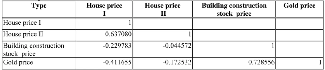
Liao et. al. (1999) points out that when the two mixed-assets of the coefficient of correlation is lower, the higher the function of diversifying risk. By the theory of portfolios, the negative correlation and the small magnitude assets are better portfolios which diversify risk. The correlation between real estate and other assets (such as building construction stocks, and gold stocks) are, in general, negative but small in magnitude. Therefore, the mixed-asset portfolios which are considered include pre-sales houses, building construction stocks and gold stocks. Table 2 shows that the coefficient of correlation among mixed assets. We found the coefficient of correlation in house price I and building construction stock price to be -0.2297, house price I and gold price is -0.4116. This indicates that mixed-assets with real estate and gold prices can reduce the fluctuation of the rate of returns of a portfolio, and reduce the risk. The coefficient correlation of house price II to building construction stock price is -0.0445, the coefficient correlation of house price II to gold price is -0.1725. We get the same result with mixed-assets of real estate and gold prices which might reduce the fluctuation of the rate of returns of a portfolio, and cut down the risk. The findings indicated that the portfolio of real estate and gold can disperse more risks on the market.
Evaluating mixed-asset Portfolios Risk in the Taiwan Residential Housing Market
Table 2: Correlation coefficient of house price I, house price II, stock price index and gold
price
Type House price I House price II Building construction stock price Gold price House price I 1 House price II 0.637080 1 Building construction stock price -0.229783 -0.044572 1 Gold price -0.411655 -0.172532 0.728556 1
2. The framework of portfolios
The mixed-asset portfolios which are considered include pre-sales houses, building construction stocks and gold stocks. The estimation of the rate of return of portfolios is shown in formula 2: T t=1 R W = R N i=1 τ i i τ P,
∑
, , ,………, (2)whereRp,t:rate of return of portfolio at t time
Wi:weight ; Ri,t:rate of returns of assets i at t time
We assume the investing net value of NTD 10 million in the mixed-asset portfolio with four scenarios. In the first scenario, the ratios of investments are 100%, 0% and 0. In the second scenario, the ratios of investments are 50%, 25% and 25%. In the third scenario the ratio of investments are 25%, 50% and 25%. In the fourth scenario the ratio of investments are 25%, 25% and 50%, where pre-sale house price have two kinds of house prices which are house price I and house price II. Table 3 proposes the mixed-asset ratio of portfolio investment.
Table 3: The ratio of portfolios under the four types of scenarios
Scenarios Pre-sales house Building construction stock Gold stock First scenario 100% 0% 0% Second scenario 50% 25% 25% Third scenario 25% 50% 25% Fourth scenario 25% 25% 50%
The scenarios proposed what the 100%, 50%, 25% of portfolios might be in real estate. The ratio in the first scenario is regarded as a benchmark. In the second scenario, we consider it as more ratio portfolio on real estate. In the third scenario, we treat it as more ratio portfolio on building construction stock. And in the fourth scenario there is more ratio portfolio on gold stock.
Table 4 shows the rate of return and risk of three kinds of investment assets. According to the MVC criterion, the expected rate of return of pre-sale houses are greater than the expected rate of return of building stock, and the risk of pre-sale houses is smaller than the risk of building stock. The expected rate of return of gold stock is greater than the expected rate of return of building stock. The risk of the gold stock is smaller than the risk of building a stock. The expected rate of return of gold stock is greater than the expected rate of return of pre-sale houses, but the risk of the gold stock is greater than the risk of pre-sale houses. So, according to the MVC criterion, the pre-sale houses are a good investment tool, and building construction stock is a poor investment tool.
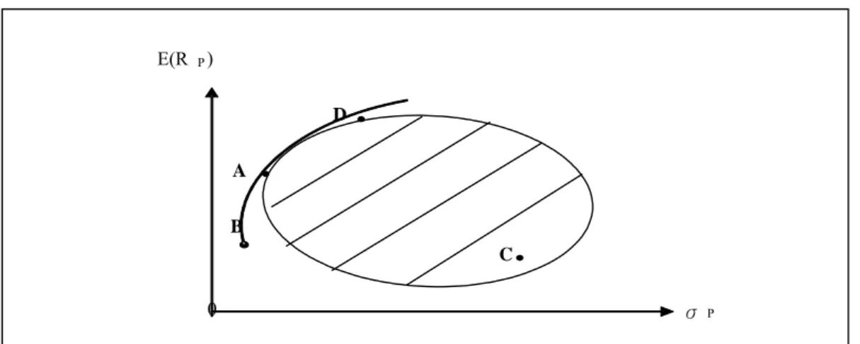
According to the efficient frontier portfolio theory, the following are pre-sale house price I, house price II, building construction stock and gold stock with four representatives of A, B, C and D. Figure.5 shows the efficient frontier and possible area of portfolio depend on the rate of return and variance of three investment assets A, B, C and D within the possible area of the portfolio.
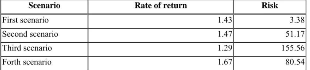
Table 4: Rate of return and risk of three investment assets
Investment assets Pre-sale house house price I (A) Pre-sale house house price II (B ) Building construction stock (C) Gold stock (D) Rate of return (Average) 1.99 1.43 0.74 2.26 Risk(Variance) 3.30 3.38 469.11 71.97
Figure 5: Efficient frontier and possible area of the portfolio
4. The results of estimate return and risk of portfolio by the Mean-Variance Criteria
(1)We estimate the rate of return and risk mixed by house price I, building construction stock price index and gold price
Table 5 shows the estimated rate of return and risk by house price I, building construction stock price and gold price under four kinds of scenarios. The results show when investments are more in proportion with pre-sale houses, then the rate of return is great and its risk is less. Otherwise, when investments are more in proportion with building stock, then the risk is greater.
Table 5: Portfolio risk by house price I, building construction stock price index and gold
E(R P) D A B C 0 σP
Evaluating mixed-asset Portfolios Risk in the Taiwan Residential Housing Market
prices under four kinds of scenario
Scenario Rate of return Risk
First scenario 1.99 3.30
Second scenario 1.75 47.53 Third scenario 1.43 152.40 Fourth scenario 1.81 78.27
(2)Estimated rate of return and risk by house price II, building construction stock price index and gold price
Table 6 shows that the estimated rate of return and risk by house price II, building construction stock price and gold price under four kinds of scenarios. The results are similar to the house price I model.
Table 6: Portfolio risk by house price II, building construction stock price index and gold
price under four kinds of scenarios
Scenario Rate of return Risk
First scenario 1.43 3.38
Second scenario 1.47 51.17 Third scenario 1.29 155.56 Forth scenario 1.67 80.54
When we fixed the ratio on gold stock among scenario II and III we found that the greater the ratio portfolio on real estate, the less portfolio risk we have. However, the more ratios put on building construction stock, the more portfolio risk we encounter. Meanwhile, we fixed the ratio on real estate among scenario III and IV we found that the greater the ratio portfolio on gold stock, the less portfolio risk we have. However, the more ratios we place on building construction stock, the more portfolio risk we obtain.
5. The result of estimate value at risk
Condition (1) Estimate value at risk by house price I, building construction stock price index and gold prices
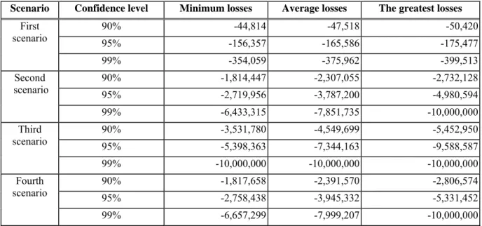
Table 7 exhibits that the use of the Historical Simulation Method results in value at risk for house price I, building construction stock prices and gold stock prices in the four-scenarios. In the assumption of investing a net value of 10 million, the mixed-asset portfolio of pre-sale houses, building construction stock and gold stock, at 95% confidence level, and holding one quarter, in the first-scenario (the ratio of investments are 100%, 0% and 0%) we estimate that the average losses reach NT 165,586 dollars. In the second scenario (the ratio of investments are 50%, 25% and 25%) the average losses are up to NT 3,787,200 dollar. In the third scenario (the ratio of investments are 25%, 50% and 25%) there are NT 7,344,163 dollars. In the fourth scenario (the ratio of investments are 25%, 25% and 50%) defined to be NT 3,945,332 dollars. The findings indicated that if we allocated more ratios in pre-sale houses,
then the market risk is less, otherwise when we invest more proportion of building construction stock, then the risk is greater.
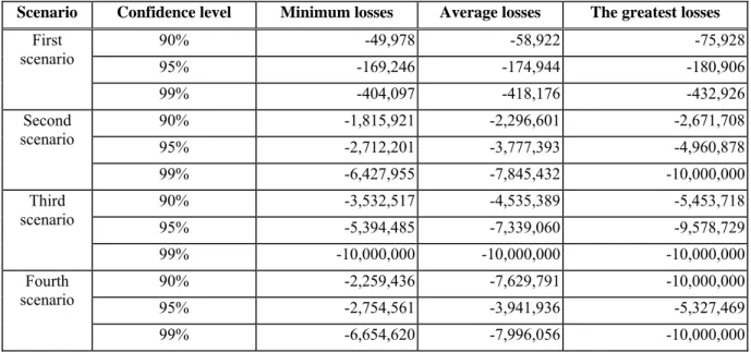
Condition (2) Estimate Value at risk by house price II, building construction stock price index and gold
Table 8 established the value at risk by using the historical simulation method in mixed asset portfolios of house price II, building construction stock prices and gold stock prices. The following are the four-scenarios with data from the 1st quarter of 2001 to the 4th quarter of 2003. The results assume investing net value of 10 million in the portfolios, at 95% confidence level, and holding one quarter.
In the first scenario (the ratio of investments are 100%, 0% and 0%) we estimate average losses to be up to NT 174,944 dollar. In the second scenario (the ratio of investments are 50%, 25% and 25%) the average losses are estimated at NT 3,777,393 dollars. In the third scenario (the ratio of investments are 25%, 50% and 25%) we estimate average losses to be NT 7,339,060 dollars. In the fourth scenario (the ratio of investments are 25%, 25% and 50%) we reach average losses of NT 3,941,936 dollars. The findings indicated same results as the above condition (1).
We compared the criteria of MVC and the smallest value at risk. This empirical study found the same results with regard to the portfolios. However in the latter part of the study we computed the value of risk, and we can further adjust the portfolio return.
Table 7: The four-scenario portfolio value at risk of condition (1)
Scenario Confidence level Minimum losses Average losses The greatest losses
90% -44,814 -47,518 -50,420 95% -156,357 -165,586 -175,477 First scenario 99% -354,059 -375,962 -399,513 90% -1,814,447 -2,307,055 -2,732,128 95% -2,719,956 -3,787,200 -4,980,594 Second scenario 99% -6,433,315 -7,851,735 -10,000,000 90% -3,531,780 -4,549,699 -5,452,950 95% -5,398,363 -7,344,163 -9,588,587 Third scenario 99% -10,000,000 -10,000,000 -10,000,000 90% -1,817,658 -2,391,570 -2,806,574 95% -2,758,438 -3,945,332 -5,331,452 Fourth scenario 99% -6,657,299 -7,999,207 -10,000,000
Note:This table estimates value at risk; the data sample period is from the 1st quarter of 2001 to the 4th quarter of 2003. We have calculated its minimum loss, average loss and the greatest loss.
Evaluating mixed-asset Portfolios Risk in the Taiwan Residential Housing Market
Table 8: The four-scenario portfolio value at risk of condition (2)
Scenario Confidence level Minimum losses Average losses The greatest losses
90% -49,978 -58,922 -75,928 95% -169,246 -174,944 -180,906 First scenario 99% -404,097 -418,176 -432,926 90% -1,815,921 -2,296,601 -2,671,708 95% -2,712,201 -3,777,393 -4,960,878 Second scenario 99% -6,427,955 -7,845,432 -10,000,000 90% -3,532,517 -4,535,389 -5,453,718 95% -5,394,485 -7,339,060 -9,578,729 Third scenario 99% -10,000,000 -10,000,000 -10,000,000 90% -2,259,436 -7,629,791 -10,000,000 95% -2,754,561 -3,941,936 -5,327,469 Fourth scenario 99% -6,654,620 -7,996,056 -10,000,000
Note:Same as the note in table 7
CONSIDERATIONS AND CONCLUSIONS
1. Considerations
In our study we had limitations on the time series data sample, Taipei-area and the individual buyer-investor, such that the resulting findings might be a constraint. We suggested some cautions as follows:
(1) The study period of time series sample is limited, because we used methods of measurement risk to estimate value at risk of financial goods or other derivative financial goods, the holding period is daily data, but for the estimated value at risk of real estate, this text holding period is quarterly data. The concept of estimated value at risk depends on the fluctuation of risk. It is not easy to capture the fluctuation of risk, and we need the caution of viewing the results with a more conservative manner. (2) This study mixed three kinds of investment asset portfolios such as pre-sale house,
building construction stock and gold stock, however, in practice, real estate is a long-run investment asset, and building construction stock and gold stock are short-long-run investment assets. We may not reach the value at risk right away to indicate the fluctuation of risk in the stock market.
(3) The main goals of incorporating a building construction stock price in this exercise are to serve as a comparison between direct and indirect investments. The direct investment indicate the real estate such as pre-sale houses, the indirect investment represents stock of Building constructions. The second thought is the theory of portfolios. The correlation between real estate and other assets (such as building construction stock, gold stock) are, in general, negative but small in magnitude. Therefore, the mixed-asset portfolios which are considered include pre-sales houses, building construction stock and gold stock. Table 4 shows the return correlation between model I house prices and building construction stock prices as -0.23. The return correlation between model II house prices and building construction stock prices are -0.04. Both indicate the function would work on risk diversification, the
mixed-asset portfolios might be considered between pre-sales houses and building construction stock. However, the empirical results found the contradictory function on risk diversification. It might not apparently select the building construction stock on the mixed-asset portfolios.
2. Conclusions
This study examines the entire efficient frontier for the mixed-asset portfolios consisting of five asset groups: pre-sale house price I, pre-sale house price II, building construction stock and gold stock for the sample period of the 1st quarter of 1985 to the 4th quarter of 2003 for approximately 76 quarterly data. We computed the value at risk of portfolio by the Historical Simulation Method under the four types of investment scenario. We applied the Mean-Variance Criteria to estimate rate of return and risk of portfolio.
The results found that when we allocate more proportion in pre-sale houses, the risk is lower; otherwise when we invest more proportion in the building stock, the risk is higher. For the mixed assets of portfolio in house price I, building construction stock and gold stock we assumed investing a net value of $10 million NT, at a 95% confidence level. The first condition results show that lower average losses, the first scenario (the ratio of investments are 100%, 0% and 0%) reached NT 165,586 dollars, and the higher third scenario (the ratio of investments are 25%, 50% and 25%) to NT 7,344,163 dollars.
Meanwhile, the second condition result (replacement on house price II) reached the lowest average losses in the first scenario (the ratio of investments are 100%, 0% and 0%) to $NT 174,944, and the highest in the third scenario (the ratio of investments are 25%, 50% and 25%) estimate to $NT 7,339,060. The mixed-asset portfolio with real estate investment was considered as a hedging instrument. The study results point out that as the ratio approaches 100% in pre-sale houses; the value at risk of investment is minimal. As the ratio reaches 50% in building stock, the value at risk of investment is the greatest. The results demonstrate that as we allocated more proportion in pre-sale houses, then the risk is less, otherwise as we put more proportion on building construction stock, then the risk is greater.
【Note】the meaning of “pre-sale house” data set:There are two house market systems in
Taiwan - one is the pre-sale housing market, the other is the existing housing market. The pre-sale system is like a forward or future market to sale in the future. The existing house trade system is similar to spot market to sale in a time period. Taiwan's pre-sale housing industry takes a special forward trading system. Normally, developers will start selling house units once blueprints are approved by the government. Home buyers will make the purchase decision based on the information given and a model home is built by the developers. 10% down payment is typically required. 20% of the total price will be paid similar to an instalment during the construction period. The remaining 70% payment will be set up by a bank as a mortgage for twenty years, effective at the time when the usage permit is issued by the housing regulation agency. This trading system provides high financial leverage to both the builders and buyers and also increases the market trading momentum. We choose the average price of a pre-sale house in our study.
Evaluating mixed-asset Portfolios Risk in the Taiwan Residential Housing Market
Chang, C.O (1996) Real estate investment, decision making and analysis, Hue-Tai Publishers (in Chinese).
Chow, D.S; Sha, D P; Chang, D C; Ching, Y K; Ko, G F (2002) The benchmark for risk management :
value at risk, Gi-Sung Publishers(in Chinese).
Hendershott, P. H. and Hendershott, R. J.(2002)On measuring real estate risk, Real Estate Finance,
Winter, 35-40.
Hon, Y.F.(2002) The study on value at risk evaluation modelling---the case study on the management
of agricultural investment portfolio, Unpublished MSc Thesis, Department of MBA, National
Ping-Tong University of Science and Technology(in Chinese).
Huang, C Y and Lin, V C C (2004) A study of evaluating investment risk on the housing market, 13th
Annual Chinese Society of Housing Studies Conference Proceedings, 13 January 2004, Sin-Su (in
Chinese).
Huang, C Y and Lin, V C C (2004) A study of evaluating investment risk-factors on the housing market, 2nd Annual Society of Land Studies Conference Proceedings, 25-26 September 2004, Taipei (in Chinese).
Huang, D.Y (2001) Value at risk: the new standard for market risk control, translated from Jorion Philippe, Taiwan Financial Training Institute (in Chinese).
Huang, E Y (2000) The value at risk evaluation of recreation investment---the case study on leisure
hotel, Unpublished MSc Thesis, Graduate School of Architecture and Urban Design, Chaoyang
University of Technology (in Chinese).
Jiang, Y.S.(2000) The evaluation of investment portfolio risk: the application on new simulation
method, Unpublished MSc Thesis, Department of MBA, National Cheng-Chin University(in
Chinese).
Lia, L.H. (1996) The study on the housing investment return rate, Unpublished MSc Thesis, Department of Land Economics, National Cheng-Chin University (in Chinese).
Liao, S S; Lee, A Y; Mei, C P (1999) The Principle of real estate investment, Hua-Tai Publishers (in Chinese).
Liu, W G; Chang, S Y; Chrang, L G (2000) The choice of the best investment in different cycle status,
The Journal of Taiwan Land Finance Quarterly, 37(4), 45-67(in Chinese).
Shung, W.H.(1995) The effect of the risk factors on real estate return and its sensitivity analysis, Unpublished MSc Thesis, School of Business, National Taiwan University(in Chinese).
Tuan, Y.S.(1992) The relationship study on real estate investment return and risk, Unpublished MSc Thesis, Department of MBA, National Taiwan University of Science and Technology(in Chinese). Wheaton, W. C.(2002)On measuring real estate risk: a reply, Real Estate Finance, Winter, 41-42. Wheaton, W. C.; Torto, R. G.; Sivitanides, P. and Southard, J.(1999)Evaluating risk in real estate,
Real Estate Finance, Summer, 15-22.
Wheaton, W. C.; Torto, R. G.; Sivitanides, P.; Southard, J. A.; Hopkins, R. E. and Costello, J. M. (2001)Real estate risk: a forward-looking approach, Real Estate Finance, Fall, 20-28.