An Incremental Learning Approach to
Motion Planning with Roadmap Management
*TSAI-YEN LI AND YANG-CHUAN SHIE
Department of Computer Science National Chengchi University
Taipei, 116 Taiwan
Traditional approaches to the motion-planning problem can be classified into solu-tions for single-query and multiple-query problems with the tradeoffs on run-time com-putation cost and adaptability to environment changes. In this paper, we propose a novel approach to the problem that can learn incrementally on every planning query and effec-tively manage the learned road-map as the process goes on. This planner is based on pre-vious work on probabilistic roadmaps and uses a data structure called Reconfigurable Random Forest (RRF), which extends the Rapidly-exploring Random Tree (RRT) struc-ture proposed in the literastruc-ture. The planner can account for environmental changes while keeping the size of the roadmap small. The planner removes invalid nodes in the road-map as the obstacle configurations change. It also uses a tree-pruning algorithm to trim RRF into a more concise representation. Our experiments show that the resulting road-map has good coverage of freespace as the original one. We have also successful incor-porated the planner into the application of intelligent navigation control.
Keywords: incremental learning, motion planning, probabilistic roadmap management, reconfigurable random forest, planning for dynamic environments
1. INTRODUCTION
The motion-planning problem has been well studied in the last three decades. The basic problem, called the path problem or the piano-mover’s problem, is about find-ing a collision-free path for a robot movfind-ing in a workspace cluttered with obstacles [22]. The developed techniques for solving this problem has been shown to be well applicable to many domains other than robotics such as computer animation [12], assembly main-tainability [7], intelligent navigation interfaces [19], and drug designs [23]. According to [2], most path planners consist of two phases: preprocessing and query phases. In the preprocessing phase, the planning problem is converted into abstract data structures such as graphs that will be searched later for a feasible path in the query phase. The percent-age of running times for the two phases might vary greatly for different planners. For example, in the Randomized Path Planner (RPP) [3], most time is spent in the query phase while in the Probabilistic Roadmap Method (PRM) planner [11], most time is spent in building a roadmap in the preprocessing phase.
Depending on how a planner is used, one can classify the planning problems into two categories: single-query and multiple-query problems. In the single-query problem, one does not assume anything about previous queries, and the planner always starts to Received March 31, 2005; revised November 11, 2005; accepted December 22, 2005.
Communicated by Chin-Teng Lin.
answer every query from scratch. On the other hand, in multiple-query problems, one usually assumes that the environment does not change often and multiple queries will be issued for the same environment. In this case, the planner can afford to spend more time on preprocessing such that the queries afterward can be answered more quickly. Choos-ing an appropriate planner for a given problem remains a state of art requirChoos-ing human judgment.
In this paper we propose a unified path-planning approach that can be used in an ei-ther single-query or multiple-query problem. The planner is well suited for a single-query problem, and it learns the given environment incrementally as the planner is called over time. The planner is as efficient as other single-query planners and the performance gets improved when the learning process goes on. It adopts a data structure, called Rapid- exploring Random Tree (RRT), has been shown to be an effective roadmap representa-tion [15, 16]. We have extended this structure to a more flexible one, called Reconfigur-able Random Forest (RRF). This data structure allows us to modify the roadmap by re-moving invalid nodes as the obstacle configurations change at run time. In addition, the planner is designed to trim unnecessary nodes in RRF periodically so that the roadmap can be kept slim. We have chosen the application of intelligent navigation interface to demonstrate the effectiveness of this approach.
The rest of the paper is organized as follows. We will first review related work in the next section and then review the RRT structure, the RRT-Connect algorithm, and present our unified approach with the RRF data structure in section 3. In the fourth sec-tion, we will extend the planner to maintain a concise roadmap in a changeable environ-ment. Experimental settings, results, and analysis will be given in section 5. In section 6, we will describe the considerations on applying this planning approach to the application of intelligent navigation interface. Finally, we will conclude our work in the last section.
2. RELATED WORK
One can obtain an introduction to the general motion-planning problem or a survey of approaches in Latombe’s book [18]. Generally speaking, early research focuses on developing theoretical foundation and complete solutions for the problem [22]. For ex-ample, A* or Best-First Planning (BFP) are all efficient complete search algorithms that take the distance to the goal as a heuristic to systematically search the grid space. How-ever, under the curse of dimensionality, this type of solution dooms to be impractical for problems involving high-dimensional search spaces. In the last decade, several re-searches start to look for practical solutions that can be applied to wider arrange of ap-plications despite they usually lack completeness [3, 11].
The randomized planners are the popular approaches along this direction. The early RPP planner is a typical single-query planner utilizing artificial potential fields as the search heuristic. In contrast, the PRM planner is a typical multiple-query planner that uses a great portion of time to construct a representative roadmap for later queries. For this type of method, the way that the sampled configurations are selected greatly affects the planning results. Variations of sampling strategies have been proposed for a generic or a specific problem [1, 5, 10]. The work in [20] uses visibility information to produce a smaller roadmap. In recent years, one form of randomized roadmap called RRT has been
shown to be effective in solving several difficult problems by being able to explore the freespace evenly [15, 16].
The RRT structure has been used as a tool to construct motion planers with various strategies. For example, a single-RRT planner called RRT-ExtExt and a bidirectional planner called RRT-ExtCon have been proposed in [9, 17]. RRT-ExtCon, also called RRT-Connect in [14], is a single query planner found to be more effective for holonomic motion planning problems than RRT-ExtExt. In fact, some early work of 3D motion planning has also shown that bi-directional search is more efficient [13]. In addition to being efficient, these RRT-based planners have been shown to be probabilistic complete, which means that the probability of connecting the initial and goal configurations, if one exists, approaches one when the number of added nodes in RRT’s become infinity [17]. In addition to being probabilistic complete, [8] proposed a planner utilizing an accessi-bility graph to establish resolution complete.
Several planners in the literature took a learning approach [4, 6, 11, 21]. In one of the early papers proposing the idea of probabilistic roadmap, roadmap was used as a way to learn the freespace [21]. They observed sharp learning curves when the roadmap got denser. However, the number of sampled configurations for an acceptable success rate remains an empirical setting. In [6], a planner called ERPP uses the local minima learned in an RPP-based planner to build a roadmap for a static environment. The work in [4] uses a genetic algorithm to evolve critical configurations, called landmarks, for freespace connectivity. The RRT-based planners are incremental in nature because of the way that it explores the search space. However, most of them are designed to solve a single-shot query problem. In this paper, we aim to learn the search space incrementally by taking advantage of RRT’s constructed in earlier queries.
3. BUILDING INCREMENTAL ROADMAP
The basic path-planning problem is to find a collision-free path for a robot amongst obstacles in a given environment. The set of all possible configurations q for the robot define the so-called Configuration Space (C-space for short), denoted by C. Let Cfree de-note the open subset of collision-free configurations in C. The path-planning task is to find a continuous curve in Cfree connecting an initial configuration, qi, and a goal con-figuration, qg.
3.1 The RRT-Connect Planning Algorithm
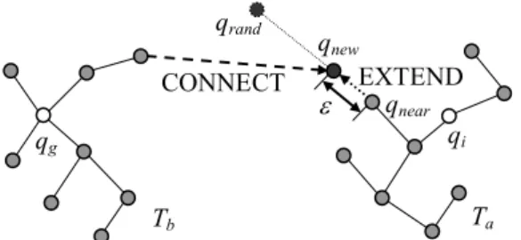
The Rapidly-exploring Random Tree (RRT) was introduced in [15] as an efficient data structure to explore Cfree. Its main difference from traditional probabilistic roadmaps is on that RRT grows outward from a tree although configurations are sampled ran-domly in the freespace. As depicted in Fig. 1, the growing process starts by selecting a random configuration, qrand, as the growing direction. The nearest configuration, qnear, in the current RRT to qrand is determined, and a new configuration, qnew, that is ε-distance away from qnear, is computed and added into the RRT. This process is called EXTEND. In [14], an efficient single-query planning algorithm, called RRT-Connect, uses RRT as the main data structure to connect the given initial and goal configurations (qi and qg).
qrand qnew qnear qi Tb EXTEND CONNECT ε qg Ta
Fig. 1. Two RRT’s use EXTEND and CONNECT to merge into one tree.
Two RRT’s, rooted at qi and qg, respectively, are used to connect to each other. At each step of the growing process, a random configuration qrand is sampled in the freespace. One RRT uses the EXTEND procedure to add to itself a new configuration, qnew, while the other RRT uses another procedure called CONNECT to grow (EXTEND) toward qnew as much as possible. If CONNECT can bring the RRT to reach qnew, then the two RRT’s have been successfully connected and a feasible path is returned. Otherwise, the two RRT’s swap to allow them to grow in the other direction.
3.2 The Incremental Learning Algorithm: RRF_CONNECT
Since the RRT-Connect planner is a single-query planner, it always starts from scratch for applications requiring multiple queries. However, we think the freespace ex-plored in previous planning queries could be very useful in the following ones. Therefore, we extend the RRT-Connect algorithm to take advantage of the previous learned knowl-edge about the freespace to save time in future queries. Since previously learned RRT’s are kept for future uses, the data structure becomes a forest consisting of multiple RRTs. We called this forest, Reconfigurable Random Forest (RRF). It is reconfigurable because the trees in the forest can be merged, split, or pruned in the planning process.
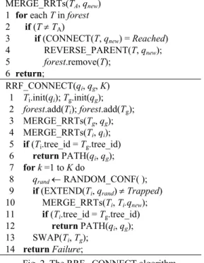
Fig. 2 shows the RRF_CONNECT planning algorithm. The algorithm assumes a global data structure called forest to store the list of currently maintained trees. A main subprocedure used in RRF_CONNECT is called MERGE_RRTs. This procedure tries to connect each tree in the forest, except for the currently considered tree TA, to the desig-nated new configuration, qnew, via the CONNECT procedure. The tree is merged with TA if the connection is successful. In the RRF_CONNECT algorithm, after the trees rooted at qi and qg are initialized, we first call the MERGE_RRTs procedure to see if we can connect the two configurations to the forest without adding additional configurations. If this is not successful, a randomly sampled configuration, qrand, will be generated to ex-tend Ti, and MERGE_RRT will then be called again. This process will repeat until the Ti and Tg are merged (success) or a predefined maximal number of sample configurations is reached (failure).
4. ROADMAP MANAGEMENT
As the learning process goes on, the RRF structure might need to be updated for a few reasons. First, if the obstacle configurations are changeable at run time, then there
MERGE_RRTs(TA, qnew)
1 for each T in forest 2 if (T ≠ TA)
3 if (CONNECT(T, qnew) = Reached)
4 REVERSE_PARENT(T, qnew); 5 forest.remove(T); 6 return; RRF_CONNECT(qi, qg, K) 1 Ti.init(qi); Tg.init(qg); 2 forest.add(Ti); forest.add(Tg); 3 MERGE_RRTs(Tg, qg); 4 MERGE_RRTs(Ti, qi); 5 if (Ti.tree_id = Tg.tree_id) 6 return PATH(qi, qg); 7 for k =1 to K do 8 qrand ← RANDOM_CONF( );
9 if (EXTEND(Ti, qrand) ≠ Trapped)
10 MERGE_RRTs(Ti, Ti.qnew);
11 if (Ti.tree_id = Tg.tree_id)
12 return PATH(qi, qg);
13 SWAP(Ti, Tg);
14 return Failure;
Fig. 2. The RRF_ CONNECT algorithm.
should be a way to invalidate certain portion of the forest. Second, there should be a way to trim unnecessary nodes as the forest grows. Keeping a tidy roadmap not only saves space but also the time required to search for a path.
4.1 The Incremental Learning Algorithm: RRF_CONNECT
The assumption of static environment restricts the application domain of road-map-based methods. In general, when the environment changes, the roadmap needs to be reconstructed. However, there exist applications where obstacles in the environments need to be moved but not constantly or frequently. For these scenarios, a major portion of the roadmap might still remain valid and useful for future queries. One can simply re-move invalid nodes after the obstacle changes and reconstruct the RRF structure.
We use the following process to reconstruct RRF after the obstacle configuration changes. First, we compute the candidate nodes whose configurations fall inside the bounding box of the obstacle’s new configuration. Second, we perform collision checks on these nodes to find the list of invalid ones to be removed. Third, for each invalid node, we check if their children are also in the invalid list. If not, then the subtree rooted at each of these child nodes will be trimmed off and becomes a new tree in RRF.
In the above update process, the first step may contain example-specific procedure to compute the bounding box of obstacles in C-space. The second step is the most time- consuming one since it involves collision detections to find invalid nodes. However, for time-critical applications, we think this step could be totally skipped by assuming that all nodes are invalid without sacrificing the correctness of the planning result for the
fol-lowing reasons. First, these nodes are selected under a necessary condition. The list con-tains a conservative list of candidate nodes. Second, if the obstacle is currently moving, its bounding box could contain nodes that will become invalid sooner or later. Third, since the RRT structure tends to grow the tree toward unexplored area, the extra space cleaned up due to the imprecise update can be filled up quickly in the future learning process. Examples of this update process will be given in the next section.
4.2 Forest Pruning
As the learning process goes on, the number of nodes added into RRF increases sig-nificantly. Although the more nodes in a roadmap, the better they can capture the overall structure of freespace. However, as the number of nodes increases to some degree, the performance of the planner might be worsen due to the large roadmap size. As a result, it is desirable to prune RRF to make it a more concise representation. In Fig. 3, we show an example of pruning an RRF from a dense roadmap (2,675 nodes, Fig. 3 (a)) to a tidier one (70 nodes, Fig. 3 (b)).
(a) (b)
Fig. 3. (a) An example of RRT (projected into the 2D workspace) and (b) an example of pruned RRT from (a).
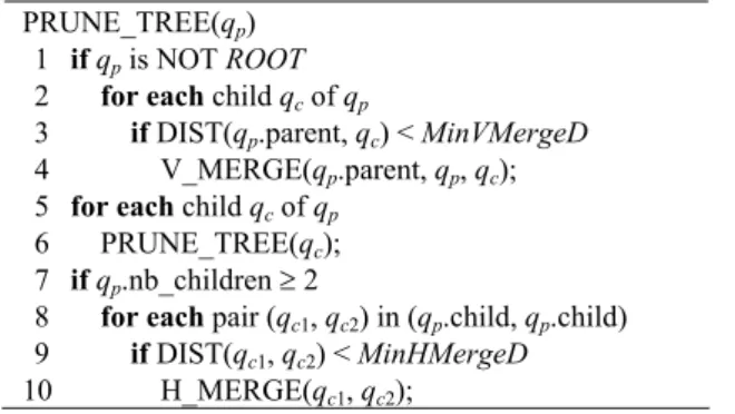
PRUNE_TREE(qp)
1 if qp is NOT ROOT
2 for each child qc of qp
3 if DIST(qp.parent, qc) < MinVMergeD
4 V_MERGE(qp.parent, qp, qc);
5 for each child qc of qp
6 PRUNE_TREE(qc);
7 if qp.nb_children ≥ 2
8 for each pair (qc1, qc2) in (qp.child, qp.child)
9 if DIST(qc1, qc2) < MinHMergeD
10 H_MERGE(qc1, qc2);
Fig. 4. The PRUNE_TREE algorithm for pruning a given tree to a more concise representation. The PRUNE_TREE algorithm that is used to prune the trees in an RRF is listed in Fig. 4. A tree is considered too dense vertically or horizontally if there exists a node too close to its grandparent node or to its sibling nodes, respectively. In this algorithm, we traverse the given tree in post order, where a node is examined after its subtrees are
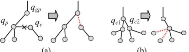
trav-ersed. When a tree is traversed, we remove nodes that are considered redundant to the structure of the tree. When examining a node (qp), we first check if the distance between each of its child nodes (qc) and its parent node (qgp), in some user-specified metric, is less than some limit, MinVMergeD, and there exists a collision-free straight-line path be-tween them. If the above conditions are met, we perform a vertical merge (V_MERGE) operation that makes the qc node connect to the qgp node directly instead of to the qp node, as shown in Fig. 5 (a). Since the qp node must have children to satisfy the above condi-tions, it must be an interior node in a tree. However, if the qp node becomes a leaf node after its children are all relinked to its parent, then it is deleted from the tree. Second, we check if the distance between any ordered pair of child nodes (qc1 and qc2) is less than some limit, MinHMergeD, and all of qc1’s child nodes, if any, can be moved to qc2 with collision-free links. If so, we perform a horizontal merge (H_MERGE) operation to move the links, and qc1 is deleted from the tree, as shown in Fig. 5 (b).
qp qc
qgp
qc1 qc2
(a) (b)
Fig. 5. (a) Vertical and (b) horizontal merges of RRT.
5. EXPERIMENTS
The aforementioned planner has been fully implemented in Java. The planning times reported in this paper were collected from experiments running on a regular PC with a K6-3 400 MHz processor. The size of the C-space (x, y, θ) for all examples shown in this paper is 128 × 128 × 100. The roadmaps depicted in this section are actually 2D projections of 3D C-space into the 2D workspace.
5.1 Forest Pruning
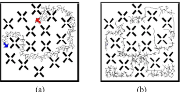
Among several tested examples, a basic path-planning example with an arrow- shaped robot in static environments is shown in Fig. 6. The workspace in Fig. 6 (a) is a 2D environment, and the configuration space is 3D. For easier visualization, the gener-ated RRF roadmap is projected onto the workspace in Fig. 6 (b). The number of sampled nodes and the planning time are 699 and 0.2 seconds, respectively. The example assumes a clean start with no pre-built roadmap. In our experiments, we continued to issue a great number of random planning queries for the same static environment to see how the later one can take advantage of the roadmap learned earlier. Two snapshots of the incremental roadmap construction process are shown in Fig. 7. The roots of the trees in RRF are de-picted with solid dots. The RRF in Fig. 7 (b) contains seven trees. As the number of plan-ning queries increase, the number of nodes in RRF increases to 2359 and the number of trees reduces to two only, as shown in Fig. 7 (c). As the number of queries increases in Fig. 7 (d), the roadmap becomes denser but the two trees still cannot be connected due to
(a) (b)
Fig. 6. An example of (a) found path in a 2D workspace and (b) the generated roadmap (projected onto the 2D workspace) for finding the path in (a).
(a) (b) (c) (d) Fig. 7. Snapshots of a growing RRF (projected into workspace)
the difficult area (narrow passage) indicated in the circles. The planning times for the example will be reported in a later subsection.
5.2 Example for Environments with Obstacle Configuration Changes
We have implemented the algorithm in section 4.1 to allow configuration changes of environmental obstacles. An example illustrating the idea of reconfigurable forest is shown in Fig. 8. The example starts with no pre-built roadmap (Fig. 8 (a)) and after 1,000 planning queries, the RRF ends up with a dense roadmap consisting of a single RRT of 2,962 nodes (Fig. 8 (b)). Then, we moved the obstacles on the lower-right corner to the center of the workspace. The roadmap is updated with the principles described in section 4.1, and the update process takes only about 50 ms. About 300 invalid nodes are detected and removed from the RRF, resulting in 22 new trees as shown in Fig. 8 (c). The roots of these trees, surrounding the moved obstacle, indicate where the forest is split. After an-other 500 random planning queries, the empty area that was originally occupied by the obstacle is quickly and evenly filled with new nodes, as shown in Fig. 8 (d). In this as-pect, the RRT structure, compared to other roadmap representations, demonstrates its strength in exploring unvisited area and therefore is more appropriate for managing roadmaps in such a dynamic scenario.
5.3 Experiments on Forest Pruning
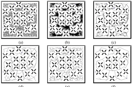
We use the example shown in Fig. 9 to illustrate the effects of the forest pruning process. The RRF roadmap shown in Fig. 9 (a) contains 5,974 nodes in total. According
(a) (b) (c) (d)
Fig. 8. An example of how RRF is updated in an environment where obstacles may be moved at run time.
(a) (b) (c)
(d) (e) (f)
Fig. 9. Experimental results on forest pruning for RRF with different parameter settings. to the PRUNE_TREE algorithm in section 4.2, two types of merges might be applied to RRF to reduce its size. To observe the effect of each type of operation, we only perform the vertical-merge operation that attempts to reduce the hierarchy of RRF by removing interior nodes. After 741ms of computation, we can reduce the number of nodes to 3412 as shown in Fig. 9 (b). This operation has flattened the RRF, but it also results in trees that are too broad horizontally. By applying the horizontal-merge operation, which takes 291ms, we obtain an RRF consisting of 518 nodes only as shown in Fig. 9 (c). If we ap-ply the vertical and horizontal merges simultaneously as in the PRUNE_TREE algorithm, the computation time is only about 330 ms. Like most algorithms for smoothing paths generated by a path planner, the PRUNE_TREE procedure does not guarantee to result in an optimal solution at once. Instead, the procedure can be applied to an RRF repeatedly until the size cannot be further reduced. In Fig. 9 (d), we show such an example consist-ing of 200 nodes only after several iterations.
Two parameters in the PRUNE_TREE procedure are set empirically to determine the characteristics of the resulting RRF: MinVMergeD and MinHMergeD. In the figure
mentioned above, the MinVMergeD and MinHMergeD are four and two times of the ε-distance used in the EXTEND procedure, respectively. A smaller value for these mini-mal distances yields a finer but larger roadmap. In Fig. 9 (e), we show an example of a finer RRF consisting of 609 nodes with the minimal distances set to ε. Furthermore, the PRUNE_TREE procedure can be applied periodically to RRF during the learning process. Our experiments show that the number of nodes in RRF can often be further reduced as the process goes on. For example, a tidier representation of 122 nodes for the RRF can be obtained, as shown in Fig. 9 (f), after a few iterations of planning query and tree-pruning operations.
5.4 Pruning Frequency
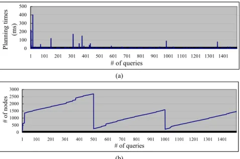
A major advantage of the proposed learning approach is that the C-space can be learned incrementally as the process goes on. Our experiments show that, as one can pre-dict, the planner learns more about the C-space when the query problem is difficult. However, the occasions are rather sparse. For example, as shown in Fig. 10 (a), the plan-ner learns about most of the C-space in the very beginning and a few times in the middle of the 1500 queries. In this experiment, the PRUNE_TREE procedure was called every 500 queries to reduce the number of nodes in RRF, and we were able to reduce it by a factor of 10, as shown in Fig. 10 (b).
0 100 200 300 400 500 1 101 201 301 401 501 601 701 801 901 1001 1101 1201 1301 1401 # of queries P lan ni ng times (ms) (a) 0 500 1000 1500 2000 2500 3000 1 101 201 301 401 501 601 701 801 901 1001 1101 1201 1301 1401 # of queries # of node s (b)
Fig. 10. Planning times and accumulated number of nodes as number of queries increases. Similarly, it is difficult to determine an optimal frequency for pruning an RRF. It takes time to prune a tree but a smaller and better roadmap representation could save time in the long run. We have done some experiments to understand the effects of pruning frequency on the number of resulting nodes as well as their coverage in the
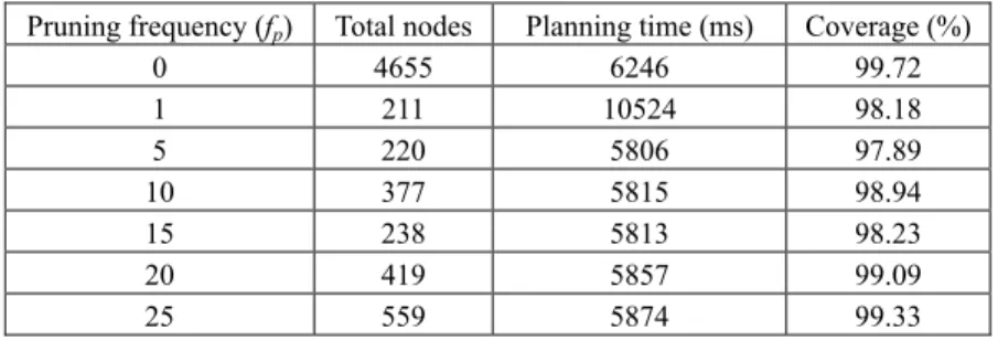
Table 1. C-space coverage rates by the pruned RRF with different frequencies. Pruning frequency (fp) Total nodes Planning time (ms) Coverage (%)
0 4655 6246 99.72 1 211 10524 98.18 5 220 5806 97.89 10 377 5815 98.94 15 238 5813 98.23 20 419 5857 99.09 25 559 5874 99.33
configuration space. The experimental data are summarized in Table 1. With different pruning frequencies (fp) ranging from 1 to 25, we can observe a factor 10 to 20 on node reduction. Except for the extreme case of performing pruning for every query (fp = 1), the overall planning times, including the RRF pruning operations, are all reduced.
According to [17], the RRT-based algorithm (single-tree or double-tree) is prob-abilistic complete. That is, the probability that the RRT initialized at the initial configu-ration will contain the goal configuconfigu-ration as a vertex approaches one as the number of vertices approaches infinity. Every planning query in our RRF algorithm can be regarded as a special case of RRT-Connect algorithm except for the additional trees constructed in the previous queries. Thus, the completeness of the RRF-CONNET algorithm is Fig. 2 is preserved. Even with the tree pruning operation introduced in Fig. 3, the only difference is on how the quality of the previously constructed roadmap (if sacrificed) contributes to the efficiency instead of completeness of the planner. In order to look into the quality of the roadmap after pruning, we have conducted a coverage test in an off-line manner. This test is done by trying a fine uniform grid of points in the C-space to see the percentage of configurations that can be connected to the roadmap with a collision-free straight-line path. As shown in the last column of Table 1, when the number of nodes in the roadmap is greatly reduced by a factor of 20, the coverage rate still can be kept above 97%. This experimental result shows that indeed we can prune a roadmap into a much slimmer one without sacrificing much its freespace coverage.
6. APPLICATION TO INTELLIGENT NAVIGATION CONTROL
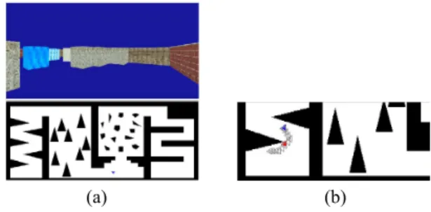
In order to demonstrate the effectiveness of the proposed planning method, we have applied the planner to the application of intelligent navigation control as proposed in [19]. In this application, the motion planner is incorporated into the control loop of the naviga-tion user interface such that a collision-free detour path is generated voluntarily when-ever the viewpoint collides with environmental obstacles. With such an assisting mecha-nism, it was reported that the navigation efficiency can be improved as much as 67 per-cent [19]. During the navigation, the motion planner is evoked many times as the view-point moves. Therefore, it is a good example application where the roadmap can be built incrementally as the robot (viewpoint in this case) moves in the workspace.
We have used the RRF planner described in this paper to generate collision-free paths during the navigation task. A maze-like scene that has been used in our experiments
(a) (b)
Fig. 11. Application of intelligent navigation: (a) a maze scene used in the experiments (b) a sam-ple path generated during the navigation.
is shown in Fig. 11 (a). The subject is asked to navigate in the 3D window, a Blaxxun3D1
VRML browser, by dragging the mouse. The 2D window, implemented as a Java Applet, shows a top view of the scene as well as the planning results. An example of such assist-ing paths (in grey) is depicted in Fig. 11 (b), where the viewpoint is modeled as a small triangle.
As mentioned in the previous section, the frequency of performing forest pruning may affect the resulting number of nodes as well as the planning time. Instead of adopt-ing a fixed prunadopt-ing frequency, in this application, we have used a strategy based on the accumulated number of new nodes to decide when to perform forest pruning. We count the number of new nodes that have been added into the forest since the last pruning. When this number exceeds some given threshold, the pruning procedure is evoked to reduce the size of the roadmap. Our experiments show that reasonably good results can be obtained with this strategy.
7. CONCLUSIONS AND FUTURE WORK
In this paper, we have described an incremental learning approach to the general path-planning problem. This approach extends the RRT-Connect algorithm proposed in the literature to maintain the RRF roadmap learned in previous queries. The new planner can manage the roadmap effectively and efficiently as the environment changes and the learning process goes on. In addition, the planner can be run in an unsupervised manner since it can always maintain a concise and representative roadmap. We believe that such a path planner can be applied to a wider range of applications in robotics and other re-lated fields.
A main drawback of this incremental learning approach is that the quality of the generated path cannot be guaranteed. Due to the nature of incremental construction and the tree structure, it is possible that the generated path is a longer detour than necessary. Therefore, there should be some mechanism to balance the trees or make useful loops in the roadmap to improve the quality of the generated paths. In addition, such an incre-mental learning approach should have a better effect in the case of large environments where a complete roadmap with good coverage is neither necessary nor efficient. A more adaptive mechanism should be designed to keep only the most relevant portion of the
roadmap in memory. We will continue investigating these issues in the future to enhance the flexibility and practicability of the planner.
REFERENCES
1. N. M. Amato, O. B. Bayazit, L. K. Dale, C. Jones, and D. Vallejo, “OBPRM: an ob-stacle-based PRM for 3D workspaces,” Robotics: The Algorithmic Perspective, 1998, pp. 630-637.
2. J. Barraquand, L. Kavraki, J. C. Latombe, T. Y. Li, and P. Raghavan, “A random sampling scheme for path planning,” International Journal of Robotics Research, Vol. 16, 1997, pp. 759-774.
3. J. Barraquand and J. C. Latombe, “Robot motion planning: a distributed representa-tion approach,” Internarepresenta-tional Journal of Robotics Research, Vol. 10, 1991, pp. 628-649.
4. P. Bessiere, J. M. Ahuactzin, E. G. Talbi, and E. Mazer, “The ‘Adriane’s clew’ algo-rithm: global planning with local methods,” in Proceedings of the IEEE/RSJ
Interna-tional Conference on Intelligent Robots and Systems, 1993, pp. 1373-1380.
5. R. Bohlin and L. Kavraki, “Path planning using lazy PRM,” in Proceedings of the
IEEE International Conference on Robotics and Automation, 2000, pp. 521-527.
6. S. Caselli and M. Reggiani, “ERPP: an experience-based randomized path planner,” in Proceedings of the IEEE International Conference on Robotics and Automation, 2000, pp. 1002-1008.
7. H. Chang and T. Y. Li, “Assembly maintainability study with motion planning,” in
Proceedings of the IEEE International Conference on Robotics and Automation,
1995, pp. 1012-1019.
8. P. Cheng and S. M. LaValle, “Resolution complete rapidly-exploring random trees,” in Proceedings of the IEEE International Conference on Robotics and Automation, 2002, pp. 267-272.
9. P. Cheng, Z. Shen, and S. M. LaValle, “RRT-based trajectory design for autonomous automobiles and spacecraft,” Archives of Control Sciences, Vol. 11, 2001, pp. 167-194.
10. D. Hsu, J. C. Latombe, R. Motwani, and L. E. Kavraki, “Capturing the connectivity of high-dimensional geometric spaces by parallelizable random sampling tech-niques,” Advances in Randomized Parallel Computing, P. M. Pardalos and S. Ra-jasekaran, eds., Combinatorial Optimization Series, Kluwer Academic Publishers, Boston, MA, 1999, pp. 159-182.
11. L. Kavraki, P. Svestka, J. C. Latombe, and M. Overmars, “Probabilistic roadmaps for fast path planning in high-dimensional configuration spaces,” IEEE Transactions on
Robotics and Automation, Vol. 12, 1996, pp. 566-580.
12. Y. Koga, K. Kondo, J. Kuffner, and J. C. Latombe, “Planning motions with inten-tions,” Computer Graphics (SIGGRAPH), 1994, pp. 395-408.
13. K. Kondo, “Motion planning with six degrees of freedom by multistrategic bidirec-tional heuristic free-space enumeration,” IEEE Transactions on Robotics and
Auto-mation, Vol. 7, 1991, pp. 267-277.
path planning,” in Proceedings of the IEEE International Conference on Robotics
and Automation, 2000, pp. 995-1001.
15. S. M. LaValle, “Rapidly-exploring random trees: a new tool for path planning,” Technical Report No. 98-11, Computer Science Dept., Iowa State University, 1998. 16. S. M. LaValle and J. J. Kuffner, “Randomized kinodynamic planning,” in
Proceed-ings of the IEEE International Conference on Robotics and Automation, 1999, pp.
473-479.
17. S. M. LaValle and J. J. Kuffner, “Rapidly-exploring random trees: progress and pros-pects,” in B. R. Donald, K. M. Lynch, and D. Rus, eds., Algorithmic and
Computa-tional Robotics: New Directions, A K Peters, Wellesley, MA, 2001, pp. 293-308.
18. J. C. Latombe, Robot Motion Planning, Kluwer, Boston, MA, 1991.
19. T. Y. Li and H. K. Ting, “An intelligent user interface with motion planning for 3D navigation,” in Proceedings of the IEEE Virtual Reality 2000 Conference, 2000, pp. 177-184.
20. C. Nissoux, T. Simeon, and J. P. Laumond, “Visibility based probabilistic roadmaps,” in Proceedings of the IEEE International Conference on Intelligent Robots and
Sys-tems, 1999, pp. 1316-1321.
21. M. H. Overmars and P. Svestka, “A probabilistic learning approach to motion plan-ning,” Technical Report No. UU-CS-1994-03, Department of Computer Science, Utrecht University, Netherlands, 1994.
22. J. H. Reif, “Complexity of the Mover’s problem and generalizations,” in
Proceed-ings of the 20th IEEE Symposium on Foundations of Computer Science, 1979, pp.
421-427.
23. G. Song and N. M. Amato, “Using motion planning to study protein folding path-ways,” in Proceedings of the 5th Annual International Conference on Computational
Biology, 2001, pp. 287-296.
Tsai-Yen Li (李蔡彥) received the B.S. in 1986 from Na-tional Taiwan University, Taiwan, and M.S. and Ph.D. in 1992 and 1995, respectively, from Stanford University. He is currently a professor and director of the Intelligent Media Laboratory (IM- Lab) in the Computer Science Department of National Chengchi University in Taiwan. His main research interests include com-puter animation, intelligent user interface, motion planning, vir-tual environment, and artificial life. He is a member of IEEE, ACM, IICM of Taiwan, and TAAI of Taiwan.
Yang-Chuan Shie (謝揚權) received the B.S. and M.S. (2000 and 2002) from Computer Science Department, National Chengchi University, Taiwan, R.O.C. He is currently a software engineer on 3D game design at InterServ Corp. His research in-terests include roadmap-based motion planning, computer game design, and virtual environment.